Three-dimensional non-local thermodynamic equilibrium radiative transfer and oxygen abundances in late-type stars

thermodynamic equilibrium radiative

transfer and oxygen abundances in

late-type stars

Anish Mayur Amarsi

A thesis submitted for the degree of

Doctor of Philosophy

of the Australian National University

© Anish Mayur Amarsi All Rights Reserved

I hereby declare that the work in this thesis is that of the candidate alone, except where indicated below or in the text of the thesis. The work was undertaken between August 2013 and September 2016 at the Australian National University (ANU), Canberra. It has not been submitted in whole or in part for any other degree at this or any other university.

This thesis has been submitted as a Thesis by Compilation in accordance with the relevant ANU policies. The main chapters are articles that are in preparation for submission to, accepted for publication in, or published in a peer-reviewed astronomy journal. The status of each article and extent of the contribution of the candidate to the research and authorship is indicated below:

• Chapter 2: Amarsi A. M., On line contribution functions and their use in ex-amining spectral line formation in 3D model stellar atmospheres, 2015, MNRAS, 452, 1612-1616. AMA developed the theory, made the necessary code developments, performed the calculations, and wrote the article.

• Chapter 3: Amarsi A. M. and Asplund M., The solar silicon abundance based on 3D non-LTE calculations, 2016, MNRAS464, 264-273. AMA made the necessary code developments, performed the calculations, and wrote the article. MA provided feedback, suggestions, and minor modifications to the text.

• Chapter 4: Amarsi A. M., Asplund M., Collet R., Grevesse N., Sauval A. J. and Barklem P. S.,The elemental composition of the Sun — IV. The solar oxygen abun-dance, in preparation. AMA made the necessary code developments, performed the calculations, and wrote most of the article. MA and RC provided feedback, sug-gestions, and minor modifications to the text. MA performed the analysis of the OH lines and wrote the corresponding section. RC wrote the section describing the model atmosphere. PSB calculated the cross-sections for the inelastic collisions of oxygen with neutral hydrogen atoms.

• Chapter 5: Amarsi A. M., Asplund M., Collet R. and Leenaarts J.,Non-LTE oxy-gen line formation in 3D hydrodynamic model stellar atmospheres, 2016, MNRAS, 455, 3735-3751. AMA made the necessary code developments, performed the calcu-lations, and wrote the article. MA, RC and JL provided feedback, suggestions, and minor modifications to the text.

• Chapter 6: Amarsi A. M., Asplund M., Collet R. and Leenaarts J., The Galac-tic chemical evolution of oxygen inferred from 3D non-LTE spectral-line-formation calculations,2016, MNRAS, 454, L11-L15. AMA made the necessary code develop-ments, performed the calculations, and wrote the article. MA, RC and JL provided feedback, suggestions, and minor modifications to the text.

• Chapter 7: Amarsi A. M., Asplund M., et al., The GALAH survey: 3D non-LTE oxygen abundances in the Galactic disk, in preparation. AMA made the necessary code developments, performed the calculations, and wrote the article. MA provided feedback, suggestions, and minor modifications to the text. The observations were taken by members of the GALAH collaboration. The data reduction pipeline and GALAH stellar parameters pipeline were developed by members of the GALAH collaboration.

• Chapter 8: Amarsi A. M., Lind K., Asplund M., Barklem P. S. and Collet R., Non-LTE line formation of Fe in late-type stars — III. 3D non-LTE analysis of metal-poor stars, 2016, MNRAS, 463, 1518-1533. AMA made the necessary code developments, performed the calculations, and wrote the article. KL, MA, PSB and RC provided feedback, suggestions, and minor modifications to the text. KL constructed and tested the model atom. PSB calculated the cross-sections for the inelastic collisions with neutral hydrogen atoms.

The candidate also made contributions to the following articles during the course of the candidature:

• Nordlander T.,Amarsi A. M., Lind K., Asplund M., Barklem P. S., Casey A. R., Collet R. and Leenaarts J.,3D NLTE analysis of the most iron-deficient star, SMSS0313-6708,2017, A&A, 597, A6.

• Lind K.,Amarsi A. M., et al., Non-LTE line formation of Fe in late-type stars — IV., in preparation.

These articles do not form a part of this thesis.

Most of the calculations presented in this thesis were performed using multi3d (

Further acknowledgements are made at the end of each article.

This thesis contains approximately 60000 words, exclusive of footnotes, tables, figures, maps, bibliographies and appendices.

Anish Mayur Amarsi October 2016

I would like to thank my supervisor Martin Asplund, advisers Remo Collet, Paul Stuart Barklem and David Yong, and collaborators Jorrit Leenaarts, Karin Lind and Thomas Nordlander, for their contributions to the content of this thesis.

The chemical compositions of the atmospheres of late-type stars, as inferred from stellar spectroscopic analyses, provide vital clues to unravelling the history of stars, galaxies, and the cosmos as a whole. However, the vast majority of stellar spectroscopic analyses make at least two assumptions that severely limit their accuracy: that stellar atmospheres are one-dimensional (1D) and hydrostatic; and that the material in the line-forming regions is in local thermodynamic equilibrium (LTE). Real atmospheres of late-type stars have convective envelopes that require a 3D time-evolving hydrodynamical treatment, and also real atmospheres are generally not in LTE.

In this thesis I develop tools for 3D non-LTE radiative transfer calculations in late-type stars, and use them to address two outstanding problems that are pertinent to oxygen, which is one of the most important elements in astronomy. First is the so-called solar mod-elling problem, wherein inferences about the structure of the Sun based on helioseismology are in significant disagreement with those inferences based on the current best estimate of the solar chemical composition (as deduced from spectroscopy) and standard solar interior models. It has been strongly argued in the literature that a higher solar oxygen abundance is needed to resolve this problem. Second is the so-called oxygen problem in metal-poor stars, wherein different oxygen abundance diagnostics give different oxygen abundances in metal-poor Milky Way disk and halo stars. In particular, this has meant that the Galactic [O/Fe] versus [Fe/H] trend, a key tracer of chemical evolution, is poorly constrained in the metal-poor regime.

I present new 3D non-LTE analyses of oxygen and silicon lines in the solar spectrum. The inferred solar oxygen and silicon abundances, 8.70±0.03 dex and 7.51±0.03 dex respec-tively, are consistent with the current canonical values to within errors, so maintaining the status quo on the solar modelling problem. I also present 3D non-LTE spectra for atomic oxygen lines across a grid of 3D hydrodynamic model atmospheres. Such a grid facilitates 3D non-LTE analyses of stars other than the Sun. With this grid I present analyses of the [O/Fe] versus [Fe/H] trend from Galactic disk and halo stars, and I demonstrate that with accurate stellar parameters and 3D non-LTE modelling, concordant results can be achieved between the two key atomic oxygen diagnostics: the [Oi] 630 nm line, and the Oi777 nm lines. Lastly, I present a 3D non-LTE analysis of Feiand Feiilines in four metal-poor benchmark stars: HD84937, HD122563, HD140283, and G64-12. I demonstrate that the 3D non-LTE iron abundances are typically 0.1 dex higher than the corresponding 1D non-LTE iron abundances. 3D effects of this order need to be accounted for if the Galactic [O/Fe] versus [Fe/H] relationship is to be properly constrained.

Disclaimer iii

Acknowledgements vii

Abstract ix

1 Introduction 1

1.1 Stellar spectroscopy of late-type stars and the cosmic chemical evolution . . 1

1.2 Model stellar spectra . . . 3

1.2.1 Overview . . . 3

1.2.2 Model stellar atmospheres . . . 5

1.2.3 Non-LTE radiative transfer . . . 11

1.2.4 Non-LTE model atoms. . . 15

1.2.5 Numerical solutions for the 3D non-LTE radiative transfer problem. 18 1.3 Oxygen abundances in late-type stars . . . 20

1.3.1 The importance of oxygen . . . 20

1.3.2 Oxygen abundance diagnostics . . . 21

1.3.3 The solar modelling problem . . . 23

1.3.4 The oxygen problem in metal-poor stars . . . 25

1.4 Aim of this thesis . . . 29

1.5 Overview of the chapters. . . 29

2 Line contribution functions 31 2.1 Introduction. . . 31

2.2 The 3D line flux contribution function . . . 32

2.2.1 Concept . . . 32

2.2.2 Derivation. . . 33

2.2.3 Rotational broadening . . . 35

2.2.4 Mean formation depth . . . 36

2.2.5 Relationship to the line flux response function . . . 36

2.2.6 Comparison to the plane-parallel line flux contribution function . . . 37

2.3 Example: 3D non-LTE spectral line formation. . . 37

2.4 Conclusion . . . 39

3 The solar silicon abundance 41 3.1 Introduction. . . 41

3.2 Method . . . 44

3.2.1 3D non-LTE radiative transfer code . . . 44

3.2.2 Model atmospheres . . . 45

3.2.3 Model atom . . . 47

3.2.3.1 Overview . . . 47

3.2.3.2 Comprehensive model atom. . . 48

3.2.3.3 Reduced model atom . . . 49

3.3 Line formation in the solar photosphere . . . 50

3.3.1 Non-LTE effect . . . 50

3.3.2 3D versus〈3D〉 . . . 53

3.3.3 Relative importance of radiative and collisional transitions. . . 54

3.4 Solar photospheric silicon abundance . . . 55

3.5 Conclusion . . . 57

4 The solar oxygen abundance 59 4.1 Introduction. . . 60

4.2 Methodology . . . 63

4.2.1 Observations . . . 63

4.2.2 Line selection . . . 64

4.2.3 Model solar atmospheres. . . 65

4.2.4 Radiative transfer codes . . . 68

4.2.6 Abundance analysis . . . 71

4.2.7 Error analysis . . . 72

4.3 Results for atomic lines . . . 74

4.3.1 [Oi] 557.7 nm . . . 75

4.3.2 Oi615.8 nm . . . 76

4.3.3 [Oi] 630.0 nm . . . 77

4.3.4 [Oi] 636.4 nm . . . 79

4.3.5 Oi777 nm . . . 80

4.3.6 Oi844.7 nm . . . 86

4.3.7 Oi926.6 nm . . . 87

4.4 Results for molecular lines . . . 88

4.4.1 OH pure rotation (∆ν = 0) lines . . . 93

4.4.2 OH vibration-rotation (∆ν = 1) lines. . . 94

4.4.3 OH first overtone (∆ν= 2) lines . . . 94

4.5 The solar oxygen abundance. . . 95

4.6 Comparison with other studies . . . 97

4.6.1 Asplund et al. (2009) and related works . . . 97

4.6.2 Ayres (2008) . . . 97

4.6.3 Caffau et al. (2008). . . 98

4.6.4 Caffau et al. (2015). . . 98

4.6.5 Socas-Navarro (2015) and related works . . . 99

4.6.6 Steffen et al. (2015) . . . 100

4.7 Conclusion . . . 101

5 Oxygen line formation in dwarfs and subgiants 103 5.1 Introduction. . . 103

5.2 Method . . . 105

5.2.1 Overview . . . 105

5.2.2 Code description . . . 106

5.2.3 Background opacities. . . 108

5.2.4 Model atom . . . 108

5.2.6 Equivalent widths, abundance corrections and abundance errors . . 112

5.3 Results. . . 114

5.3.1 Non-LTE effects . . . 114

5.3.2 3D atmospheric inhomogeneities . . . 118

5.3.3 Non-vertical radiative transfer . . . 121

5.3.4 Background UV opacity at low [Fe/H] . . . 123

5.3.5 Neutral hydrogen collisions . . . 125

5.3.6 Abundance errors. . . 126

5.3.6.1 Oi777 nm lines. . . 127

5.3.6.2 Oi616 nm line . . . 128

5.3.6.3 [Oi] 630 nm and [Oi] 636 nm lines . . . 128

5.3.7 Grids of equivalent widths and abundance corrections . . . 129

5.4 Comparison with previous 1D non-LTE studies . . . 130

5.4.1 Sitnova et al. (2013) . . . 130

5.4.2 Fabbian et al. (2009b) . . . 132

5.4.3 Ram´ırez et al. (2007). . . 132

5.4.4 Takeda (2003) . . . 134

5.5 Conclusion . . . 134

6 The Galactic chemical evolution of oxygen, part I 137 6.1 Introduction. . . 137

6.2 Calculations . . . 140

6.2.1 Model atmospheres . . . 140

6.2.2 Spectral line formation. . . 140

6.2.3 Model atom . . . 140

6.2.4 Background opacities. . . 141

6.3 Abundance corrections . . . 142

6.4 The Galactic chemical evolution of oxygen . . . 143

7 The Galactic chemical evolution of oxygen, part II 147 7.1 Introduction. . . 147

7.2.1 The GALAH data set . . . 149

7.2.2 3D non-LTE model spectra . . . 151

7.2.3 Fitting procedure. . . 153

7.3 Results. . . 154

7.4 Conclusion . . . 156

8 Iron line formation in metal-poor stars 159 8.1 Introduction. . . 159

8.2 Method . . . 162

8.2.1 Code description . . . 162

8.2.1.1 Overview . . . 162

8.2.1.2 Equation-of-state and background opacity. . . 163

8.2.1.3 Angle quadrature . . . 164

8.2.1.4 Frequency parallelization . . . 164

8.2.1.5 Loss of significance issues . . . 164

8.2.2 Model atom . . . 165

8.2.3 Model atmospheres . . . 174

8.2.3.1 3D hydrodynamic models . . . 174

8.2.3.2 1D hydrostatic models. . . 176

8.2.4 Observations . . . 177

8.2.5 Error analysis . . . 177

8.3 Metal-poor benchmark stars . . . 181

8.3.1 3D non-LTE Fe line formation . . . 181

8.3.2 1D versus 3D non-LTE line formation . . . 182

8.3.3 LTE versus non-LTE line formation . . . 183

8.3.4 Best inferred iron abundances . . . 184

8.4 Grids of non-LTE abundance corrections . . . 185

8.4.1 Non-LTE effect . . . 186

8.4.2 3D effect . . . 187

8.4.3 Comparison with Lind et al. (2012). . . 188

9 Conclusion 191

9.1 Summary of thesis . . . 191

9.1.1 Developing the tools for 3D non-LTE spectroscopic analyses. . . 191

9.1.2 1D versus 3D non-LTE spectroscopic abundances . . . 193

9.1.3 Spectroscopic stellar parameters and metallicities . . . 194

9.1.4 The solar chemical composition . . . 195

9.1.5 The Galactic chemical evolution of oxygen. . . 196

9.2 Future projects . . . 197

9.2.1 The [Si/O] and [Si/Fe] ratios in metal-poor stars . . . 197

9.2.2 The [C/O] ratio in metal-poor stars and in exoplanet host stars . . . 200

9.3 Outlook . . . 202

Introduction

1.1

Stellar spectroscopy of late-type stars and the cosmic

chemical evolution

The cosmic chemical evolution is the study of when, where, and how, the elements in the Universe were formed; in the context of our own Milky Way Galaxy, it is known as the Galactic chemical evolution (e.g. Tinsley,1980; Pagel, 1997; Matteucci,2012). This study spans from the beginning of the Universe, about 13.8 Gyr ago (Planck Collaboration et al., 2015), to the present day. Hydrogen and helium, the most abundant elements in the Universe, were formed along with trace amounts of lithium shortly after the Big Bang (e.g. Cyburt et al., 2016). From this primordial cosmic gas, the first stars were formed, about several hundred million years later (e.g. Bromm et al., 2009). While they lived, the first stars fused hydrogen and helium to make carbon, oxygen, and successively heavier “metals” (astronomy jargon for elements heavier than hydrogen and helium), all the way up to iron; as they died, in energetic supernova explosions, they made even heavier elements (stellar and supernova nucleosynthesis respectively; e.g.Woosley & Weaver,1995;

Heger & Woosley, 2002; Nomoto et al., 2013; Karakas & Lattanzio, 2014). These first stars enriched the primordial cosmic gas with metals from which the next generation of stars formed. This cycle, of gas to stars, and back to gas, repeats to the present day, with successive generations of stars forming from increasingly enriched cosmic gas, and subsequently synthesizing and releasing heavier metals back into the cosmos.

Our best understanding of the cosmic chemical evolution comes from studying the stars. The chemical compositions of, or elemental abundances1 in, the atmospheres of the stars at the present epoch closely reflects the chemical composition of the protostellar gas form which the stars formed (altered slightly perhaps by mixing of material from within the stellar interior where nucleosynthesis is ongoing; e.g.Pinsonneault,1997). By studying the

1_{Here, “abundance” shall refer to the number of nucleiN}

A of a given element A. Conventionally, this

is expressed relative to hydrogen such that logA≡log (NA/NH) + 12.

atmospheres of stars of different ages, astronomers can track the evolution of the elements through cosmic time.

Determining the chemical compositions of stellar atmospheres is more complicated than determining the chemical compositions of most other things, because astronomers cannot (yet) travel to the stars to measure them directly. Instead, astronomers infer the fun-damental stellar parameters — which include the stellar chemical compositions, masses, ages, luminosities, effective temperatures, surface gravities, rotational velocities, peculiar motions, and magnetic fields — indirectly, by observing, analysing and decrypting the starlight here on Earth. The keys to obtaining this wealth of information are the bright and dark lines present in the star’s electromagnetic spectrum: spectral lines, that are the result of emission and absorption processes that occur as light travels through the star’s atmosphere. The presence and relative intensities of different spectral lines depends sen-sitively on the star’s fundamental parameters, and not least on the chemical composition in the stellar atmosphere.

Stellar spectroscopy is the quantitative study of these spectral lines. The fundamental principle is simple: The observed spectrum of a given star is found and compared to theoretical model spectra that correspond to different fundamental stellar parameters. Ideally, a single theoretical model will best match the observed spectra; we then deduce that the parameters of that model are also the actual parameters of the star.

Not all stars are equally suited for studying the cosmic chemical evolution in this way. Late-type stars, which here shall mean stars of spectral types F, G, and K (e.g. Gray,

2008, Chapter 1), are the ideal candidates for spectroscopic studies of chemical evolution, and are the focus of this thesis. Compared to earlier-type stars of spectral types O, B, and A, FGK-type stars have longer lifetimes and are more abundant in the Galaxy. Also unlike OBA-type stars, FGK-type stars are characterized by large convective envelopes; this implies that their surface abundances are less susceptible to the effects of thermal diffusion, gravitational settling and radiative levitation (e.g. Pinsonneault,1997), so that their surface compositions are more reflective of the composition of the gas from which they formed. FGK-type stars are typically slow rotators (e.g. Fekel, 1997): this implies that their surface abundances are largely unaffected by rotational mixing with enriched material from the stellar interior (e.g.Talon et al.,1997). With less rotation, the spectra of FGK-type stars suffer from less rotational broadening, which means the absorption and emission features are better resolved and therefore easier to analyse. Compared to later-type stars of spectral later-type M, FGK-later-type stars are easier to detect and can be used to probe larger distances as they are typically brighter. The spectra of M-type stars are also more difficult to analyse because of the presence of many overlapping molecular bands.

1.2

Model stellar spectra

1.2.1 Overview

The conceptual starting point for constructing model stellar spectra (e.g. Rutten, 2003;

Hubeny & Mihalas,2014) is the radiative transfer equation, i.e. the Boltzmann transport equation for photons, which gives the intensityI at a given frequency,

1

c ∂I

∂t +n· ∇I =η−χI , (1.1)

or, assuming a steady state (∂/∂t= 0), dI

dτ =I−S , (1.2)

wherecis the speed of light andtis the time coordinate, the optical depth along the path

snis dτ =−χds, and the source functionS= _χη is given by the ratio of the emissivity to the linear extinction coefficient. Neglecting any absorption and emission effects that occur on the path between the star’s atmosphere and the astronomer’s telescope, the observed spectrum of an unresolved star is given by the astrophysical flux,

F = Z

S

I µdΩ, (1.3)

that emerges from the observed hemisphere of the star S, in spherical polar coordinates whereµ= cosθand dΩ = dµdφ;I is understood to be in the direction of the observer.

In spectroscopic analyses of late-type stars, model spectra are usually computed by solving the time-independent radiative transfer equation, Eq. 1.2, as accurately as possible through a pre-computed model stellar atmosphere, given an assortment of atomic data, such as the Einstein coefficients, photoionisation cross-sections and line-broadening parameters, that are needed to calculate χ and η, or τ and S, as well as to calculate the equation of state. The model stellar atmosphere specifies the temperature-pressure stratification. It is labelled by a set of stellar parameters: effective temperature Teff, defined via the Stefan-Boltzmann law,

L= 4πR2σ T_eff4 , (1.4)

whereσ is the Stefan-Boltzmann constant,L is the luminosity andR is the stellar radius; surface gravity logg, defined as

g= G M

whereGis the gravitational constant andM is the stellar mass; and the chemical compo-sition, typically denoted [Fe/H]2 for simplicity, with the abundances of all other elements set by scaling the solar chemical composition (Asplund et al.,2009).

Spectroscopic abundance analyses normally proceed one element at a time, wherein a set of theoretical spectra are generated for a set of abundances of the chosen element, over narrow wavelength regions that envelop the spectral lines that correspond to absorption and emission by atoms, ions, and/or molecules of that element. Changing the abundance of a given element affects the spectra directly via the quantitiesχand η(which depend on the number of absorbers and emitters), as well as indirectly via changes to the equation of state. Spectroscopic analyses can also be based on large wavelength windows containing many spectral lines associated with many different chemical species present in the stellar atmosphere, in which case the analysis may also be used to determine, for example, the effective temperatures and surface gravities of stars.

The model stellar atmosphere is fixed during the spectroscopic analysis. In principle, the changes in the abundances of the elements being analysed generally incur changes on the temperature-pressure stratification; thus the model stellar atmosphere should be varied during the analysis. In practice, at least when studying late-type stars the trace-element assumption is employed, which stipulates that variations in the abundance of the elements under consideration have a negligible effect on the model stellar atmosphere. This assumption is sometimes relaxed for iron, and occasionally for oxygen, silicon, and otherα-capture elements (elements for which the atomic mass numbers of the main stable isotopes are multiples of four, starting from 16_{O, and are produced in abundance in the} interiors of stars via fusion with theα-particle,4He; e.g.Woosley & Weaver,1995). Fixing the model stellar atmosphere drastically simplifies the spectroscopic analysis and reduces its computational cost. In particular, it permits a simplified treatment of the radiative transfer equation to be used during the construction of the model stellar atmosphere, with an accurate treatment postponed for during the spectroscopic (abundance) analysis stage.

The vast majority of spectroscopic abundance analyses make two crucial approximations (in addition to the trace-element assumption) when computing model spectra:

• The stellar atmosphere is one-dimensional (1D) and hydrostatic, and is in radiative equilibrium in the upper-most layers.

• The material throughout the stellar atmosphere satisfies Saha-Boltzmann excita-tion and ionisaexcita-tion balance, as is implied if the material is in local thermodynamic equilibrium (LTE).

2

0

1

2

3

4

5

6

0

1

2

3

4

5

6

0

1

2

3

4

5

6

x / Mm

0

1

2

3

4

5

6

y / Mm

0

1

2

3

4

5

6

0

1

2

3

4

5

6

0.4

0.5

0.6

0.7

0.8

0.9

1.0

Normalized intensity

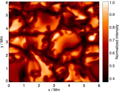
Figure 1.1: Continuum intensity at 500 nm, emerging vertically from a 3D hydrodynamic stag-germodel solar atmosphere (Collet et al.,2011a). The granulation pattern results from convection occurring beneath the solar surface, with most of the emergent intensity arising from the hot, bright granular upflows and less arising from the cool, dark intergranular downflows.

These approximations greatly reduce the time it takes to compute the model spectra, but at the cost of accuracy. The errors incurred can dominate the overall error budget, with the potential to be larger than those incurred from “observational errors” that may include, for example, photon noise, stray light, continuum placement, and unidentified blends in the observed spectra, as well as from other “modelling errors” errors including those prop-agated forward from the atomic data and adopted stellar parameters (e.g.Asplund,2005). The main idea of this thesis is to relax the 1D and LTE approximations, simultaneously and in a self-consistent way.

1.2.2 Model stellar atmospheres

High spatial resolution observations of the star nearest to us, the G-type dwarf we call the Sun, reveal that its surface is “granulated” (Fig.1.1), a phenomenon that is attributed to convection occurring just below the visible surface (e.g Herschel, 1801; Dawes, 1864;

−4

−2

0

2

2500

5000

7500

10000

12500

−4

−2

0

2

log

τ

2500

5000

7500

10000

12500

T / K

−4

−2

0

2

log

τ

2500

5000

7500

10000

12500

T / K

Procyon

T

= 6522 K

log

(g/cm s

) = 4.00

[Fe/H] = 0.00

1D MARCS

<3D>

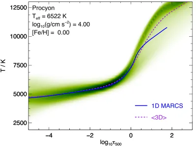
Figure 1.2: The temperature stratification in a 3D hydrodynamic_stagger model atmosphere of the solar-metallicity turn-off star Procyon (Collet et al.,2011a). Also shown is the temperature stratification from a theoretical 1D hydrostaticmarcsmodel atmosphere (Gustafsson et al.,2008), which is in close agreement with the mean temperature stratification (〈3D〉) in the line-forming regions (−4_.logτ500.0).

becomes stable against convection, (dictated by the temperature gradient, as per the Schwarzschild criterion;Schwarzschild,1906). The gas cools, and falls downwards through the atmosphere in dark, narrow intergranular downflows. An important consequence of this phenomenon is a net outwards convective energy flux, that supplements the net outwards radiative energy flux. While high spatial resolution images of stars other than the Sun have not yet been acquired, it is hypothesized that late-type stars in general display analogous stellar surface granulation phenomena, as they are all characterized by outer convective envelopes; this hypothesis is strongly supported also by computer simulations of the outer layers of these types of stars (e.g.Nordlund & Dravins,1990;Asplund et al.,1999;Ludwig et al.,2009; Freytag et al., 2012; Beeck et al., 2013b,a; Magic et al., 2013a;Trampedach et al.,2013).

−

4

−

2

0

2

2500

5000

7500

10000

12500

−

4

−

2

0

2

log

τ

2500

5000

7500

10000

12500

T / K

−

4

−

2

0

2

log

τ

2500

5000

7500

10000

12500

T / K

G64

−

12

T

= 6428 K

log

(g/cm s

) = 4.20

[Fe/H] =

−

3.00

1D MARCS

<3D>

Figure 1.3: The temperature stratification in a 3D hydrodynamic_stagger model atmosphere of the metal-poor turn-off star G64-12 (Collet et al., 2011a). Also shown is the temperature stratification from a theoretical 1D hydrostaticmarcsmodel atmosphere (Gustafsson et al.,2008), which is significantly larger than the mean temperature stratification (〈3D〉) in the line-forming regions (−4_.logτ500.0).

King,2003) of mass conservation,

∂ρ

∂t =−∇ ·(ρv) , (1.6)

momentum conservation,

∂(ρv)

∂t =−∇ ·(ρv v)− ∇p−ρ∇Φ− ∇ ·σ , (1.7)

and energy conservation,

∂e

∂t =−∇ ·(ev)−p(∇ ·v) +qrad+qvisc. (1.8)

564.54

564.56

564.58

0.5

1.0

1.5

564.54

564.56

564.58

λ

/nm

0.5

1.0

1.5

Relative intensity

3D non

−

LTE resolved

3D non

−

LTE averaged

<3D> non

−

LTE

Figure 1.4: Spatially-resolved Si_i 564.6 nm line profile at disk-centre on a snapshot of a 3D hydrodynamic solar model atmosphere, the spatially averaged profile, and the profile that emerges vertically from the horizontally- and temporally-averaged snapshot (denoted <3D>), in which velocity fields and microturbulence are neglected. In the 3D hydrodynamic model atmosphere the line is shifted, skewed, and strengthened to various degrees across the surface. The averaged profile displays a net blue-shift and broadening.

qrad = −∇ ·Frad where Frad is the radiative flux. Modern 3D time-dependent hydrody-namic model atmospheres of late-type stars are mostly of the “box-in-a-star” variety in which the fluid equations are solved for a small box that is taken to be representative of the entire atmosphere (e.g. Freytag et al., 2012; Magic et al., 2013a). For magnetically-active atmospheres the fluid equations above must be supplemented with the equations of magneto-hydrodynamics (MHD; e.g.V¨ogler et al.,2005). In general, small-scale magnetic fields may have a systematic effect on the temperature-pressure stratifications and on the inferred elemental abundances (e.g.Fabbian & Moreno-Insertis,2015) but the effect seems to be small, at least in the case of iron, carbon, nitrogen and oxygen abundances in the Sun (Moore et al.,2015;Shchukina & Trujillo Bueno,2015;Shchukina et al.,2016). Non-LTE spectroscopic analyses based on 3D MHD model stellar atmospheres are beyond the scope of this work.

for convection: time derivatives (∂/∂t ≈0) and fluid motions (v ≈ 0). In this limit the continuity equation Eq. 1.6, is trivially satisfied, while the momentum equation, Eq.1.7, reduces to the well-known condition of hydrostatic equilibrium,

dp

dz =−ρ

dΦ

dz , (1.9)

after viscous terms are also neglected. In practice, bulk vertical flows are sometimes included via an extra turbulent pressure arising from the the horizontal average of the

ρv v term in the momentum equation: pt =ρ vt2, where vt is a characteristic fluid speed

(e.g. Gustafsson et al.,2008). The energy equation, Eq.1.8, is also affected. With fluid motions neglected, convective energy transport, the dominant mode of energy transport in the deeper layers of the atmosphere, has to be approximated by adding an extra convective flux Fconv to the radiative fluxFrad via the parameterized Mixing-Length Theory (MLT;

B¨ohm-Vitense,1958;Henyey et al.,1965). The energy equation thus becomes d

dz(Frad+Fconv) = 0. (1.10)

In the upper layers the convective flux is neglected and radiative equilibrium (qrad = 0) is enforced.

The incomplete description of convection inherent in 1D hydrostatic model atmospheres poses a problem for spectroscopic analyses of late-type stars. Conceptually it helps to identify two distinct issues, associated with a) the mean temperature stratification and b) the atmospheric inhomogeneities associated with granulation (although in reality these issues are not perfectly decoupled).

The temperature stratifications of 1D model stellar atmospheres show large deviations from the “correct” temperature stratification, as gauged by that found in the mean (horizontally- and temporally-averaged) 3D model stellar atmospheres (hereafter denoted

〈3D〉; e.g. Magic et al., 2013b). These deviations can be attributed to the approximate treatment of convective energy transport employed in the energy equation, Eq. 1.8, as discussed above. The largest discrepancies are in the upper layers of metal-poor stellar stellar atmospheres, where the energy equation is controlled by the balance between ra-diative heating effected by spectral lines and adiabatic cooling of the expanding granular fluid; i.e. radiative equilibrium does not hold (e.g. Asplund et al., 1999). In metal-poor turn-off stars the temperatures of the 1D hydrostatic model atmospheres (which neglect adiabatic cooling) are too hot in the upper layers by several hundred or even thousands of kelvin (compare Fig. 1.2with Fig. 1.3). The corresponding errors in the inferred elemental abundances can easily reach 0.5 dex, at least within the assumption of LTE (e.g.Asplund et al.,1999).

the predicted strengths, shapes and doppler shifts of spectral lines (e.g. Dravins et al.,

1981; Dravins & Nordlund, 1990a; Asplund et al., 2000); in particular, the line profiles predicted by 1D and 〈3D〉 model stellar atmospheres are generally too narrow (Fig.1.4). In practice, detailed line formation calculations based on 1D model atmospheres must employ at least two more free parameters, the microturbulence and macroturbulence, to account for additional broadening by velocity variations on small- and large-scales relative to the mean free path of photons, respectively. The microturbulenceξ has dimensions of speed and acts to increase the Doppler width ∆λD of spectral lines via

∆λD=

λ c

r 2kBT

m +ξ

2_{, (1.11)}

whereλis the wavelength of the line,cis the speed of light,kBis the Boltzmann constant,

T is the kinetic temperature, and m is the mass of the particles that absorb and emit radiation (e.g. Gray, 2008, Chapter 11). The macroturbulence is usually defined as the width of some convolution function (often a Gaussian) that is applied to the emergent flux profile to model large-scale velocity variations (e.g. Gray, 2008, Chapter 17). These parameters are calibrated to the observations during the spectroscopic analysis.

One advantage that the 1D hydrostatic simulations have over the 3D hydrodynamic simu-lations is that the former are much less computationally demanding; consequently, they are able to afford a more detailed treatment of radiative transfer. The current state-of-the-art for 3D hydrodynamic simulations solve the radiative transfer equation in a simplified man-ner by using a small number of bins (typically around twelve) or multi-group methods for the opacities (e.g.Nordlund,1982;Skartlien,2000). Furthermore, the material is assumed to be in LTE (even when the subsequent spectroscopic abundance analysis is based on non-LTE radiative transfer). In contrast, 1D hydrostatic simulations can afford to sample the opacities across the spectrum, solving the radiative transfer equation in detail for of the order 105 wavelengths (e.g.Gustafsson et al.,2008), and can even afford to relax the assumption of LTE (e.g. Hubeny,1988;Short & Hauschildt,2009).

The challenges involved in computing 3D hydrodynamic model atmospheres, as well as in subsequently generating model spectra by performing detailed radiative transfer calcu-lations through them, are the main reasons for why most spectroscopic analyses are still based on 1D hydrostatic model atmospheres. Computing a single 3D hydrodynamic model atmosphere requires sophisticated, parallelized codes (e.g. V¨ogler et al., 2005; Gudiksen et al.,2011;Freytag et al.,2012;Magic et al.,2013a) and a considerable amount dedicated computational resources. For practical applications to stellar spectroscopy, a grid of such models is required; extended grids were not available until very recently (e.g.Ludwig et al.,

2009; Magic et al., 2013a). Once given a grid of 3D hydrodynamic model atmospheres, performing detailed line formation calculations on them is O(nx×ny×nt×nφ) more

777.2 777.3 777.4 777.5 0.6

0.7 0.8 0.9 1.0

777.2 777.3 777.4 777.5

λAir/nm 0.6

0.7 0.8 0.9 1.0

Normalized intensity

log

ε

=8.7

3D LTE

3D non−LTE

Observed

Figure 1.5: Theoretical LTE and non-LTE spectra for the OI 777 nm triplet lines at disk-centre from a 3D hydrodynamic model solar atmosphere, assuming a fixed oxygen abundance. This plot was made using the model atom presented in Chapter5, adoptingSH= 1.25. The lines are weaker when LTE is imposed, because the lines suffer from photon losses. The observed spectrum from the Kitt Peak disk-centre solar atlas (Brault & Neckel,1987;Neckel,1999) is also shown.

computational cost scaling with the resolution in the horizontal dimensions xand y, tem-poral dimensiont, and azimuthal angleφ. This scaling is even greater for non-LTE analyses because the steep temperature gradients associated with the atmospheric inhomogeneities tend to increase the number of iterations required to reach convergence, and can in some cases render convergence virtually impossible.

1.2.3 Non-LTE radiative transfer

The quantitiesχandη, orτ andS, that appear in the radiative transfer equation, Eq.1.2, depend on the populations of absorbers and emitters. The populationsnin different states

i at a given location in the model atmosphere are governed by the equations of kinetic equilibrium,

∂ni

∂t +∇ ·(niv) =

X

j

njPj i−ni

X

j

which follow directly from the Boltzmann transport equation (e.g. Hubeny & Mihalas,

2014, Chapter 9). In practice, this system of equations is simplified by assuming a steady state (∂/∂t = 0), by decomposing the transition probabilities P into a collisional part

C and a radiative partR, and by assuming that collisional and radiative processes act on timescales much shorter than the timescales of fluid motions:

X

j

nj (Cj i+Rj i) =ni

X

j

(Ci j+Ri j) ; (1.13)

these are the equations of statistical equilibrium. For closure, the total number of particles must be specified (and varied during the abundance analysis).

The radiative transition probabilities couple the material to the radiation field. In the unified notation of Rybicki & Hummer(1992),

Ri j =

Z Z ₁

h ν (Ui j+Vi j)IdνdΩ, (1.14)

where h is the Planck constant, ν is the frequency, and Ω is the solid angle. For bound-bound transitions with i corresponding to a lower energy state than j the U and V co-efficients are related to the Einstein coco-efficients Aj i for spontaneous emission, Bj i for

stimulated emission, and Bi j for radiative absorption via,

Ui j = 0, (1.15)

Uj i =

h ν

4πAj iφi j, (1.16)

Vi j =

h ν

4πBi jφi j, (1.17)

Vj i =

h ν

4πBj iφi j, (1.18)

where, under the assumption of complete frequency redistribution (e.g.Rutten,2003), the line profileφis assumed to be the same for the three different cases of absorption/emission (for a generalisation to the more general case of partial frequency redistribution, see Uiten-broek, 2001). For bound-free transitions with i corresponding to a lower ionisation state thanj the U and V coefficients are related to the photoionisation cross-section αi j via,

Ui j= 0, (1.19)

Uj i=

2h ν3

c2 exp (−β h ν)αi jneΦi j, (1.20)

Vi j=αi j, (1.21)

whereneis the electron number density and Φ is the Saha-Boltzmann function, which can be defined via the LTE populations n∗,

Φi j =

n∗_i nen∗j

. (1.23)

In this notation, the total extinction and emissivity, given by the sum of extinctions and emissivities of the individual radiative transitions plus a fixed background contribution denoted using “bg”, is given by

χ=X

j>i

(njVj i+niVi j) +χbg, (1.24)

η=X

j>i

niUi j+ηbg. (1.25)

If, instead, the material is in LTE, Boltzmann statistics can be employed (e.g. Hubeny & Mihalas, 2014, Chapter 9). The LTE populations are derived from the Boltzmann excitation equation,

n∗_i,I N_I∗ =

gi,I

ZI

exp (−β i,I), (1.26)

and the Saha ionisation equation,

N_I∗₊₁ne

N_I∗ =

2 Λ3

ZI+1

ZI

exp (−β χI). (1.27)

The Maxwell-Boltzmann distribution specifies the momentap of all particles:

fpd3p=

β

2π m

3₂

exp−βp·p

2m

d3p. (1.28)

Here,ilabels the energy state and I labels the ionisation stage; g is the statistical weight andZ is the partition function;is the energy with respect to ground andχis the ionisa-tion potential;neis the electron number density,β= 1/kBT and Λ =h/

√

2πm kBT is the thermal de Broglie wavelength. There are further equations describing the molecular equi-librium in LTE; for diatomic molecules this is perfectly analogous to the Saha ionisation equilibrium (e.g.Barklem & Collet,2016). As for the equations of statistical equilibrium, the total number of particles must be specified (and varied during the abundance analysis).

the sum of collisional transition probabilitiesCi j; pfrom collisions with different perturbers p, which are given by Ci j; p=nphσi j; pvpi, where the angled brackets indicate averaging over the Maxwell-Boltzmann distribution andσi j; p is the collisional cross-section for that particular transition. The usual perturbers considered to be important in late-type stars are electrons and hydrogen atoms, on account of their high speeds and high abundances, respectively (e.g. Barklem, 2016a); the relative importance of hydrogen collisions to elec-tron collisions scales as nH/ne, and grows towards lower metallicities (because metals are the main electron donors in stellar atmospheres).

There are two fundamental non-LTE “effects”, that describe how the radiative transitions drive the material away from Saha-Boltzmann equilibrium, and therefore from LTE (e.g.

Hubeny & Mihalas,2014, Chapter 14). For simplicity, consider the statistical equilibrium condition for a fixed number of two-level atoms N = n1 +n2 in a fixed background atmosphere:

n1 C1 2+B1 2J¯

=n2 C2 1+A2 1+B2 1J¯

, (1.29)

where ¯J is the intensity averaged over the solid angle, weighted by the line profile.

• Photon losses: if the radiation is weaker than thermal, J < B(T) where B(T) is the Planck function, then the left hand side is too small when LTE is assumed. The statistical equilibrium is such that n1 increases and n2 decreases, compared to the LTE expectation; the absorption line is stronger in non-LTE (Fig. 1.5). This usually occurs for strong lines (or active continua) that have a significant influence on the radiation field, in the absence of a strong, super-thermal background radiation field. Physically, the absorption line strengthens in non-LTE because a significant fraction of the emitted photons scatter large distances away and maybe even escape from the star altogether, instead of being reabsorbed.

• Photon pumping: if the radiation field is stronger than thermal,J > B(T), then the left hand side is too large when LTE is assumed. The statistical equilibrium is such thatn1decreases andn1 increases, compared to the LTE expectation; the absorption line is weaker in non-LTE. This usually occurs for weaker lines (or passive continua) when there is a strong super-thermal background radiation field, such as in the Wien regime (in late-type stars, this corresponds to the ultra-violet). In the Wien regime the Planck function decays rapidly with temperature, whereas in reality the photons are scattered rather than destroyed. This means a largeJ −B(T) excess develops. This is particularly efficient in metal-poor stars, where the lack of metal lines and continua increases the J−B(T) excess.

0

1

2

3

4

5

6

7

−

20

−

15

−

10

0

1

2

3

4

5

6

7

∆

E / eV

−

20

−

15

−

10

log

10

(<

σ

v>/cm

3

s

−

1

)

Drawin

Barklem, Belyaev et al.

T = 4000K

Figure 1.6: Magnesium excitation rate coefficients for collisions with hydrogen atoms, calculated using the recipe of Drawin(1968, 1969) as formulated byLambert (1993), compared to detailed quantum mechanical calculations from Belyaev et al. (2012) and integrated over the Maxwell-Boltzmann distribution by Barklem et al.(2012), at a fixed temperature. The seven lowest states of magnesium are considered (ignoring fine structure; see Belyaev et al., 2012); thus there are (7×6)/2 = 21 transitions considered. The recipe ofDrawin(1968,1969) is only able to predict 5 excitation rate coefficients, and only 4 to an acceptable level of accuracy; it fails for the 16 other transitions because they are radiatively-forbidden.

and Eq. 1.29then imples that the whole system (material plus radiation field) are approx-imately in LTE (after employing the Einstein relations; e.g. Hubeny & Mihalas, 2014, Chapter 5); this typically holds in the very deep layers of the atmosphere as well as in the stellar interior where the mean free path of photons is small (e.g.Rutten,2003). Real atomic systems have the added complication of having many levels, each coupled with ra-diative and collisional transitions of different intrinsic strengths, that compete to determine the overall statistical equilibrium.

1.2.4 Non-LTE model atoms

coefficients and photoionisation cross-sections that couple them, and as the line broadening parameters that are needed to determine the line profiles φ that appear in Eq.1.15 to Eq. 1.18. In contrast, LTE radiative transfer only requires the energy levels, Einstein coefficients, and line broadening parameters of the spectral line being analysed. This makes LTE radiative transfer calculations considerably more straightforward.

The model atoms used in this thesis were constructed from mainly three online databases. The NIST Atomic Spectra Database (Kramida et al., 2015) is a very useful repository of laboratory energy levels and Einstein coefficients. The Kurucz Smithsonian Atomic and Molecular Database (Kurucz,1995) supplements this laboratory data with theoretical calculations for energy levels and radiative transitions that have not been measured by ex-periment; such data are often necessary for constructing comprehensive model atoms. The Topbase Atomic Database (Cunto & Mendoza,1992;Cunto et al.,1993) contains theoret-ical energies, Einstein coefficients, and photoionisation cross-sections, calculated for the Opacity Project (Hummer & Mihalas, 1988; Seaton,1995) strictly under the assumption of LS coupling. Most model atoms used in contemporary non-LTE calculations employ photoionisation cross-sections from Topbase.

With the existence of extensive databases such as these, the energy levels, Einstein co-efficients and photoionisation cross-sections that go into a model atom can be complete and reasonably accurate. The situation is less Arguably the most pressing need is for accurate and complete collisional cross-section data. As discussed above, the collisional transitions compete against the radiative transitions, driving the material towards LTE. It is therefore crucial to have a reliable estimate of these cross-sections. Laboratory results (e.g.Fleck et al.,1991) are sparse in the literature, so most model atoms are entirely built from theoretical collisional cross-sections.

The current state-of-the-art computations of electron collisional cross-sections use close-coupling methods such as the R-matrix method (e.g. Burke et al., 1971;Burke & Robb,

1976;Berrington et al.,1974,1978), the B-spline R-matrix method (e.g. Zatsarinny,2006;

Zatsarinny & Bartschat, 2013), and the convergent close-coupling method (e.g. Bray & Stelbovics,1995,1992;Schweinzer et al.,1999), in order of increasing computational cost. These methods are based on modern atomic structure calculations, that expand the elec-tronic wavefunction for the colliding system in terms of the wavefunctions of the isolated atom and the electron; this naturally takes into account the specific quantal properties of the states under consideration.

between the initial and final state. As they employ the Bethe approximation, they are also functions of the oscillator strength, and thus fail when the oscillator strength is un-defined; for such radiatively-forbidden transitions a common way to proceed is to adopt an arbitrary “effective” oscillator strength, which is far from ideal.

Low-energy hydrogen collisions are more complicated than electron collisions, because here the nuclear motion couples to the electron motion, with the effect that the electronic wavefunction of the colliding system generally cannot be expressed as an expansion of the wavefunctions of the isolated atom and the hydrogen atom (e.g.Barklem,2016a). Calcu-lations of the collisional cross-sections therefore rely on more complex molecular structure calculations of the quasi-molecule that forms during the collision, instead of more basic atomic structure calculations. The state-of-the-art is based on quantum chemistry calcula-tions of the potential energy surfaces for the quasi-molecule and of the couplings between nuclear and electronic motion, combined with the Born-Oppenheimer approximation for the collision dynamics. Such calculations exist for collisions of hydrogen atoms with lithium (Belyaev & Barklem,2003), sodium (Belyaev et al.,1999,2010), and magnesium (Guitou et al.,2011;Belyaev et al.,2012). Very recentlyBarklem(2016b) developed a new approx-imate model based on linear combinations of atomic orbitals for the molecular structure, and the Landau-Zener model for the collisional dynamics; this approximate model should be accurate enough for practical non-LTE applications (Chapter 4and Chapter 8).

In the absence of detailed quantum-mechanical hydrogen collisional cross-sections, the recipe ofDrawin(1968,1969), as formulated byLambert(1993) orSteenbock & Holweger

(1984), is usually employed. This recipe, based on the classical electron-ionisation cross-section ofThomson (1912), has only a limited bearing on the actual quantum mechanical physics involved (Barklem et al.,2011). Comparisons with the models above for lithium, magnesium and sodium suggest that the recipe of Drawin (1968, 1969) has a tendency to overestimate the collisional cross-sections. It is customary to apply a calibrated global scale factorSHto the cross-sections (e.g.Asplund,2005), however such an approach cannot rectify any relative errors between different transitions. As the recipe of Drawin (1968,

1969) is proportional to the optical oscillator strength, it makes no predictions about radiatively-forbidden transitions; for such transitions an arbitrary “effective” oscillator strength must again be adopted (Fig. 1.6). Finally, there is currently no analogous recipe for determining the cross-sections for charge transfer reactions (A + H→A++ H−; e.g.

1.2.5 Numerical solutions for the 3D non-LTE radiative transfer prob-lem

The non-LTE radiative transfer equation, Eq. 1.2, is non-linear in the intensities. It is also non-local, since the radiation field couples together parts of the atmosphere that are separated by distances of up to the order the mean free path of photons. The non-linear, non-local nature of the problem makes it a formidable one to solve. Compared to 1D radiative transfer in 1D hydrostatic model atmospheres, the situation is worse for 3D radiative transfer in 3D hydrodynamic model atmospheres where there are four extra dimensions (x,y,t, φ), and where steep gradients associated with inhomogeneities can drive very large non-LTE effects that hamper convergence. If the material is simply assumed to be in LTE, however, the populations and consequently the quantities χ, η,

τ andS can be solved analytically; the LTE radiative transfer problem then reduces to an innocuous first-order linear ordinary differential equation, whose solution is trivial.

The 3D non-LTE radiative transfer code used in this work is multi3d (Botnen &

Carls-son,1999;Leenaarts & Carlsson,2009); other codes in use by the community include, for example,muga(Auer et al.,1994;Trujillo Bueno & Fabiani Bendicho,1995;Fabiani

Ben-dicho et al., 1997), RH (Uitenbroek, 2000;Holzreuter & Solanki,2012), nlte3d (

Praka-paviˇcius et al.,2013;Steffen et al., 2015), phoenix/3d (Hauschildt & Baron,2014), and porta (Stˇˇ ep´an & Trujillo Bueno, 2013). These codes all take an iterative approach to tackling the non-LTE problem. First, they perform, for a fixed set of populations, a for-mal solution of the monochromatic radiative transfer equation through the atmosphere, sampling the solid angle using of the order tens or hundreds of rays and sampling fre-quency space using thousands (Chapter4 and Chapter 5), tens of thousands (Chapter 3

and Chapter 8), or hundreds of thousands (Hauschildt & Baron,2014), of frequency points. Second, they update the populations given the formal solution for the radiation field, using the equations of statistical equilibrium, Eq. 1.13. Iterations proceed until consistency is obtained between the populations and the radiation field. A final formal solution is then computed to obtain the emergent stellar spectrum.

Almost all modern non-LTE codes use some variant of the MALI preconditioning scheme developed byRybicki & Hummer (1991, 1992). To illustrate this, consider the equations of statistical equilibrium, Eq. 1.13, in the unified notation of Sect.1.2.3,

X

j

njCj i+

X

j

nj

Z Z ₁

h ν (Uj i+Vj i)IdνdΩ

=ni

X

j

Ci j+ni

X

j

Z Z 1

In ordinary “lambda” or Picard’s iterations (e.g.Trujillo Bueno & Fabiani Bendicho,1995), the intensity is expressed in terms of the emissivity η and an operator Ψ:

I = Ψ h

η†

i

; (1.31)

here † indicates a quantity determined from the previous iteration. This scheme is dis-favoured because it tends to stabilise rather than converge (e.g.Auer,1991). In the MALI scheme ofRybicki & Hummer(1991,1992), the intensity is preconditioned, by subtracting from Ψ an approximate operator Ψ∗:

I = Ψ∗[η] + (Ψ−Ψ∗) h

η†

i

. (1.32)

In multi3d, and in many other codes, Ψ∗ is chosen to be the diagonal part of Ψ corre-sponding to Jacobi iterations; this approach is cheap to compute, is simple to implement in massively-parallel programs, and has been shown mathematically to have good conver-gence properties (Olson et al.,1986).

Physically, the operator Ψ describes how a pulse originating from a given depth point spreads across all depths (e.g. Hubeny, 1992). During lambda iterations, the solution is communicated on distances of the order a mean free path of photons after each iteration. Where this mean free path is small (such as in the cores of saturated lines; e.g. Rybicki,

1972,1984), the solution takes a long time to converge. The diagonal Ψ∗ operator guesses the true solution locally; preconditioning Eq. 1.32means that this guess is implicit in the subsequent iteration. Consequently with the Jacobi scheme the solution propagates over larger distances per iteration, and thus convergence is improved (e.g. Olson et al.,1986).

The formal solution is usually either based on long-characteristics or on short-characteristics (e.g.Stone et al.,1992;Heinemann et al.,2006). In its simplest form, long-characteristics involves solving the radiative transfer equation over rays drawn through each grid point that traverse the entire grid, for each frequency and direction, with boundary conditions set at the top and bottom of the model atmosphere. This approach is computationally ex-pensive, scaling as roughlyOn4_grid/3

in a (cubic) 3D grid withngridgrid points (e.g.Stone

et al.,1992;Auer,2003). For short-characteristics, as is implemented inmulti3d (Ibgui

et al.,2013), the radiative transfer equation is solved over ray segments that pass through each grid point, and that only extend as far as the faces of the closest grid cell. This has the advantage of being computationally optimal, i.e. the computational scales asO(ngrid), and of being easy to implement into domain-decomposed parallelized codes (e.g.Stˇˇ ep´an & Trujillo Bueno,2013). The disadvantage is that here the upwind intensity must be found by interpolation along the grid faces, which can make this method more diffusive than long-characteristics (e.g. Stone et al.,1992).

the three spatial dimensions), as well as parallelized over frequency space (this latter par-allelization was implemented in Chapter 8). The parallelization uses the Message Passing Interface (MPI) standard3 for distributed-memory communication, which permits simula-tions to be run on hundreds or even thousands of CPUs. This makes multi3d suitable for practical and realistic non-LTE spectroscopic analyses based on large, realistic model atoms.

Non-LTE codes developed for use with 1D hydrostatic model atmospheres such asmulti(Scharmer & Carlsson,1985;Carlsson,1986),detail(Butler & Giddings,1985), andtlusty(Hubeny,

1988) can be adapted trivially for use with 3D hydrodynamic model atmospheres, if lat-eral radiative transfer can be neglected (so that each column is treated as a separate, infinitely extended atmosphere, in the so-called 1.5D approximation; e.g. Shchukina & Trujillo Bueno,2001;Shchukina et al.,2005,2012). This approximation is discussed more in Chapter 5, in the context of Oi777 nm line formation in late-type stars.

1.3

Oxygen abundances in late-type stars

1.3.1 The importance of oxygen

Oxygen is arguably the most important and influential element besides hydrogen and perhaps helium in astronomy. It is the most abundant metal in the solar system, the Milky Way, and in the local Universe (e.g. Clayton, 2003). It consequently has a large effect on stellar structure and evolution, as a large source of opacity in stellar interiors, as a component of the energetic CNO cycle (e.g.VandenBerg et al.,2012), and as a seed for the nucleosynthesis of heavier elements (e.g.Woosley & Weaver,1995). For similar reason oxygen has a large influence on planetary atmospheres (e.g. Madhusudhan, 2012) and planetary compositions (e.g.Kuchner & Seager,2005;Bond et al.,2010), via the influence of the CO molecule on the overall molecular equilibrium. Finally, it almost goes without saying that oxygen is extremely interesting for being one of the essential elements for life as we know it (along with carbon, hydrogen, nitrogen, phosphorus and sulphur).

Oxygen abundances are useful to astrophysicists, because the nucleosynthetic origins of the element are relatively simple and well understood (e.g. Stasi´nska et al.,2012). Most oxygen forms as 16O (the primary isotope, with isotopic fraction 99.76%; e.g. Clayton,

2003), during the hydrostatic burning of helium in the interiors of stars. Massive stars (M &8M) undergo core-collapse supernovae at the end of their lives, at which point most

of this oxygen is expelled into the cosmos (e.g. Woosley et al., 2002). Lower-mass stars do not undergo core-collapse supernova at the end of their lives; the oxygen that they produce is locked up in the white dwarfs that survive them. When these white dwarfs

3

undergo type Ia supernova most of this oxygen is used as nuclear fuel (e.g.Hillebrandt & Niemeyer, 2000; Seitenzahl et al., 2013), and so is never released into the cosmos. The otherα-capture elements are similarly formed mainly in massive stars; however, they form mainly in the advanced nuclear burning stages (after the helium burning phase), which are more complicated to model and thus less well understood (e.g. Woosley et al.,2002).

Sinceαcapture elements form mainly in massive stars, the [α/Fe] versus [Fe/H] trends can be used to directly probe the cosmic chemical evolution. Empirically, [α/Fe] in Galactic disk and halo stars is seen to plateau in the regime−3.[Fe/H].−1, and monotonically decreases in the regime −1.[Fe/H].0 (e.g. Edvardsson et al.,1993;Chen et al., 2000;

Bensby et al., 2003, 2005, 2014; Fulbright, 2002; Chen et al., 2002; Reddy et al., 2006;

Nissen et al., 2007; Fuhrmann, 2008). Tinsley (1979) suggested that this reflects the more complicated nucleosynthetic origins of iron. Unlike the α-capture elements, iron is formed both by massive stars (during explosive Si burning via core-collapse supernova; e.g. Woosley et al., 2002), and by type Ia supernova of white dwarfs (e.g. Hillebrandt & Niemeyer,2000;Seitenzahl et al.,2013). The observed decline in [α/Fe] then reflects the increasing importance of type Ia supernova for chemical enrichment at later cosmic times. More quantitatively, the height of the plateau in the empirical [α/Fe] versus [Fe/H] trends contains information about the initial mass function (which describes the distribution of stellar masses at the beginning of their respective lives; e.g. Scalo, 1986; Kroupa, 2001;

Nakamura & Umemura,2001), while the “knee” in the trend around [Fe/H]≈ −1 contains information about the rate of star formation in the early galaxy (e.g.Matteucci & Brocato,

1990;McWilliam,1997,2016).

Given the importance of oxygen, it is perhaps unsurprising that there are a number of outstanding disputes surrounding oxygen abundances in late-type stars (Sect.1.3.3 and Sect.1.3.4). Partly responsible for these oxygen controversies is the lack of reliable lines that are sufficiently strong and clean (i.e. free of blending with other lines) for reliable quantitative oxygen abundance analyses (e.g.Stasi´nska et al.,2012). Morover, the oxygen diagnostics that are commonly used for abundance analyses of late-type stars are suscep-tible to 3D and/or non-LTE effects. The oxygen abundance diagnostics are discussed in detail in the following section.

1.3.2 Oxygen abundance diagnostics

radiatively-forbidden lines are sometimes discussed in the literature (e.g.Conti et al.,1967;

Altrock,1968;Lambert,1978;Mel´endez & Asplund,2008), although analyses of them are complicated by blends with multiple molecular lines. The [Oi] 557 nm line is blended with two C2 lines (e.g. Mel´endez & Asplund,2008), and the [Oi] 636 nm line is blended with two CN lines (e.g.Asplund et al.,2004); it is also located on the red wing of the the broad Cai636 nm 4p3F→4d3G auto-ionisation line (e.g.Mitchell & Mohler,1965). These two forbidden lines also form in LTE, and are also sensitive to 3D effects.

In FG-type turn-off and dwarf stars perhaps the most popular diagnostics are the high-excitation radiatively-allowed Oi777 nm lines. Although they are typically clean and strong, these lines show large departures from LTE in 1D hydrostatic model atmospheres because of photon losses (e.g.Kiselman,1993;Gratton et al.,1999;Takeda,2003;Ram´ırez et al.,2007;Fabbian et al.,2009b). The Oi777 nm lines have been extensively studied using 3D non-LTE radiative transfer in the solar spectrum (Kiselman & Nordlund,1995;Asplund et al.,2004;Pereira et al.,2009b;Prakapaviˇcius et al.,2013;Steffen et al.,2015), but, prior to this thesis, such an investigation had not been extended to other stars. The accuracy of the non-LTE modelling of these lines has been limited by poorly-known neutral hydrogen collisional cross-sections (e.g. Takeda, 2003; Allende Prieto et al., 2004), at least until very recently (see Chapter4). Other high-excitation radiatively-allowed atomic oxygen lines are less commonly used because they are usually weaker and/or are blended; they all suffer departures from LTE to varying degrees. The Oi616 nm lines show weak departures from LTE (e.g. Takeda,2003) and can be used in stars with [Fe/H]&−1.0 (e.g.Bertran de Lis et al., 2015); they are usually too weak in more metal-poor late-type stars. The Oi844 nm lines and the Oi926 nm lines show more modest departures from LTE. Analyses of these lines are complicated by blends with Feilines in the former case, and telluric lines in the latter case (e.g. Asplund et al.,2004;Caffau et al.,2008).

Electron-excitation OH lines in the ultra-violet (UV) can be used in FGK-type stars (e.g.

Israelian et al.,1998, 2001; Boesgaard et al., 1999), while vibration-rotation OH lines in the infra-red (IR) can be used in GK-type stars (Barbuy et al.,2003;Mel´endez et al.,2001;

Mel´endez & Barbuy,2002; Mel´endez,2004;Mel´endez et al.,2008). However, as molecule formation has a strong temperature dependence, these lines require a careful treatment of the model atmosphere (i.e. they are prone to 3D effects; e.g. Asplund & Garc´ıa P´erez,

1980

1985

1990

1995

2000

2005

2010

2015

8.70

8.80

8.90

9.00

1980

1985

1990

1995

2000

2005

2010

2015

Year

8.70

8.80

8.90

9.00

log

ε

Lambert 78

Anders & Grevesse 89 Grevesse & Sauval 98 Holweger 01

Allende Prieto+ 01 Asplund+ 04, 05 Caffau+ 08, 11

Asplund+ 09

Caffau+ 15 Steffen+ 15

This work

Figure 1.7: A small sample of literature values of the solar oxygen abundance as determined from spectroscopy. Today, the dispute is between a low value of around 8.69 dex (e.g.Mel´endez & Asplund,2008;Asplund et al.,2009;Pereira et al.,2009b;Scott et al.,2009), and an intermediate value of around 8.76 dex (e.g. Caffau et al., 2008, 2011; Steffen et al., 2015). Higher values have mostly been ruled out in recent years (although see e.g. Centeno & Socas-Navarro, 2008; Socas-Navarro,2015).

1.3.3 The solar modelling problem

order of tens of individual elements to just one or two (usually [Fe/H] and [α/Fe]). Any errors in the assumed solar chemical composition can therefore propagate to affect the analyses of other stars. Finally, the Sun is unique in that the spectroscopically-inferred solar chemical composition can be tested, by comparing it to the composition of other solar system material, including that of the Earth (e.g. McDonough & Sun, 1995), meteorites (e.g.Lodders et al.,2009), and comets (e.g. Lawler et al.,1989), as well as to abundances inferred via helioseismology (e.g. Basu & Antia, 2004, 2008). Large uncertainties in the spectroscopically-determined chemical composition of the Sun, for which the abundances should be best constrained, cast doubt on the abundances measured in other stars, and on any subsequent inferences about the cosmic chemical evolution that are based on stellar spectroscopy.

For these reasons, changes to the canonical solar chemical composition are highly contro-versial. With the development of 3D hydrodynamical modelling and 3D non-LTE radiative transfer methods, as well as improved atomic and molecular data, the canonical solar oxy-gen abundance has seen a significant downwards revision (Fig.1.7) from the high values of logO = 8.93±0.035 (Anders & Grevesse,1989) and logO= 8.83±0.06 (Grevesse &

Sauval,1998), to the comparatively low values of logO= 8.66±0.05 (Asplund et al.,2005) and logO = 8.69±0.05 (Asplund et al.,2009). This spectroscopic value is however dis-puted by of the order 0.07 dex (Fig. 1.7), between a low value of around 8.69 dexMel´endez & Asplund (2008);Asplund et al. (2009); Pereira et al. (2009b); Scott et al. (2009), and an intermediate value of around 8.76 dex (Caffau et al.,2008, 2011; Steffen et al.,2015); however, much higher values have mostly been ruled out. Improvements to the models similarly effected downwards revisions of the abundances of the other metals. In particular, the solar neon abundance has seen a downwards revision from logNe = 8.08 (Grevesse

& Sauval,1998), down to logNe= 7.93 (Asplund et al.,2009). The overall photospheric

mass fraction of metals was revised from Z = 0.0169 (Grevesse & Sauval, 1998) down to

Z = 0.0134 (Asplund et al.,2009).

The now widely adopted solar chemical composition, when combined with standard solar interior modelling, cannot be consolidated with inferences of the solar interior from helio-seismology (e.g.Bahcall et al.,2004;Basu & Antia,2004,2008;Basu et al.,2014;Delahaye & Pinsonneault, 2006; Pinsonneault & Delahaye, 2009; Serenelli et al., 2009; Serenelli,

2016). The discrepancies centre around three related quantities: the depth of the convec-tion zoneRCZ, the helium abundance in the convection zoneYCZ, and the sound speed as a function of depthc(R). Helioseismic measurements implyRCZ/R= 0.713±0.001 (Basu