Issues in the design of switched linear control systems:
A benchmark study
Douglas Leith, Robert Shorten, William Leithead , Oliver Mason
The Hamilton InstituteNUI Maynooth Ireland
Paul Curran
Department of Electronic and Electrical Engineering NUI Dublin
Ireland
Abstract: In this paper we present a tutorial overview of some of the issues that arise in the design of
switched linear control systems. Particular emphasis is given to issues relating to stability and control system realisation. A benchmark regulation problem is then presented. This problem is most naturally solved by means of a switched control design. The challenge to the community is to design a control system that meets the required performance specifications and permits the application of rigorous analysis techniques. A simple design solution is presented and the limitations of currently available analysis techniques are illustrated with reference to this example.
1. Introductory remarks
Recent years have witnessed an enormous growth of interest in dynamic systems that are characterised by a mixture of both continuous and discrete dynamics. Such systems are commonly found in engineering practice and are referred to as hybrid or switching systems. The widespread application of such systems is motivated by ever increasing performance requirements, and by the fact that high performance control systems can be realised by switching between relatively simple LTI systems. However, the potential gain of switched systems is offset by the fact that the switching action introduces behaviour in the overall system that is not present in any of the composite subsystems. For example, it can be easily shown that switching between stable sub-systems may lead to instability or chaotic behaviour of the overall system, or that switching between unstable sub-systems may result in a stable overall system.
In this paper we present a tutorial introduction to the design of switched linear systems. We begin by discussing how switching arises naturally in many situations. Examples include: the design of control systems for plants that are themselves characterised by switching action (i.e. plants with gears); the design of reconfigurable (fault tolerant) control systems; a switched controller that combines the advantages of several LTI controllers; and using switching to improve the transient response of adaptive control systems. We then discuss the issues in the design of such systems. Of primary practical importance are the issues of asymptotic stability, and issues concerning the realisation of switched linear controllers (and the associated transient response). Each of these issues is illustrated by means of simple illustrative examples.
analysing the stability of switched systems. In this context, a fundamental contribution of this paper is to document the limitations of these techniques and to motivate the study of theoretical issues that arise in the context of real industrial examples.
2. The Need for Switching
Switching between a number of control strategies has long been a valuable tool in the design of automatic control systems.
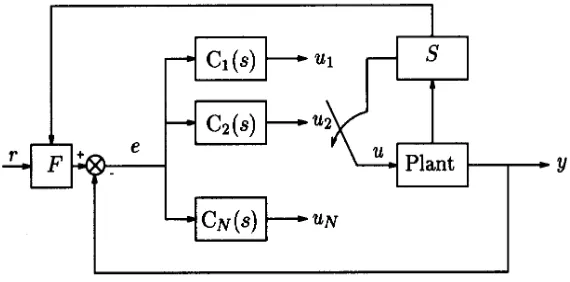
[image:2.595.160.445.232.373.2]Figure 1: Schematic of a switching system. ‘S’ denotes a supervisory algorithm that controls the
switching between the various controllers.
The need for (supervisory) switching arises for many reasons, some of which are listed below (Narendra et al., 1996, Goodwin, 2001):
(i) Plant dynamics: Many physical systems can be represented by switching or interpolating between
locally valid models. Controllers that encompass switching are often a natural method for dealing with such systems.
(ii) Performance: Switching between a number of control structures automatically results in control
systems that are no longer constrained by the limitations of linear design. It is therefore not surprising that switching based control strategies can result in algorithms that offer significant performance improvements over traditional linear control. For example, different controllers may be encoded within a single structure, resulting in a control system with enhanced functionality by exploiting the benefits of each of the constituent controllers.
(iii) Robustness: An important motivation for designing switching control strategies is to ensure robust
control performance in the presence of component failure. For example, if an operating condition changes (a sensor failure, a change in sampling rate, or even a controller failure), then a more appropriate control action may be initiated by the supervisor. In extreme cases, switching to a new controller, or even continuous switching between a number of controllers, may be required to maintain closed loop stability.
(iv) Adaptive control: Much of the recent interest in switching systems has been motivated by
(v) Decentralised design: Many complex engineering systems are designed in a decentralised manner.
Each component sub-system is usually designed in relative isolation, and the overall system is constructed by combining each of the sub-systems by means of some appropriate supervisory logic. Often, this approach leads to switched linear control systems.
(vi) Control system constraints: Constraints are a common feature of practical control systems.
Switching between several controllers is often a natural way of satisfying such constraints. Examples in this context are given in (Goodwin, 2002).
Despite the prevalence of switching based control algorithms in engineering design, such systems have only recently, in the context of the more general hybrid systems, attracted the interest of the academic community. Typically, switched linear systems are modelled by vector differential equations of the following form,
x(t0) x0, ,
u ) t ( B x ) t ( A
x= + =
where n
R ) t ( u ), t (
x ∈ and where matrices A(t), B(t), are constructed by switching between a set of
matrices. Formally we define a switched linear system, referred in the sequel to as the switching system, and its fundamental properties as follows (Shorten et. al., 2002).
The switching system: Consider the time-varying system
x ) x(t , B(t)u(t) A(t)x
(t) x
: = + 0 = 0
(1)
where n p
R
R ∈
∈ ,u(t)
x(t) and where matrices A(t), B(t), are constructed by switching between a set
of stable matrices, A(t) {A ,A ,....,A },B Rnn,
i m
×
∈
∈ 1 2
p n i
m},B R
B ,...., B , B { ) t (
B ∈ 1 2 ∈ × and where
for each time t the matrices A(t), B(t) equals one and only one matrix Ai , Bi in the above sets.
Typically the matrix pairs (Ai,Bi) are chosen such that equation (1) is bounded-input bounded-output
stable for all fixed values of t (Khalil, 1992). This corresponds to switching between a number of
stable systems. Further, we assume that once the matrices A(t), B(t) assume the values Ai , Bi they
assume these values for an interval of time τ where
> ≥τ
τ where the constant τ is arbitrarily
small and independent of i. For instance, suppose that the dynamics in (1) are given by x=Aix+Biu
over the finite time interval [t ,t 1)
+ . At time
+ γ
the system switches and the dynamics in the
following interval [t ,t 2)
1
+ + are given by x A x B u
j
j +
=
. We assume that the state vector x(t) does
not jump discontinuously at
+ γ
, and hence the initial state at time
+ γ
for x =Ajx+Bju
is the
terminal state of x=Aix+Biu
. If we further assume that u = Kix then the following convenient
representation of (1) is obtained,
0 0) x , t ( x x ) t ( A x
: = =
(2)
where A(t)∈{A1,A2,....,Am}, and Ai =Ai +KiBi. We refer to systems (1) and (2)
interchangeably as the switching system.
Associated with the switching system (1) we also define the ith constituent system, the switching
sequence SW and a switching signal
ρ
The ith constituent system: Consider the linear time-invariant system
u B x A x
: = i + i
i
(3)
with the switching system defined above. Then Σ is referred to as the i
th
The switching sequence SW: In the spirit of (Branicky, 1994) one can associate the following switching sequence with (1)
SW = (i0, t0),(i1,t1),...,(iN,tN),...,
where the SW sequence may or may not be infinite. The th switching interval is the thelement of
this sequence and defines the evolution of (1) as follows. The switching system evolves according to
u B x A
:
i
i +
=
x
i
for
1
+
< ≤t t
t , with the initial condition given by x(tγ).
The switching signal: Let (t):R→R
be a piecewise constant function, (t) {1,...,m}
∈ for all t.
Suppose that the switching sequence SW is chosen such that A(t)=A (t)for all t. Then, (t)
is said to
be a switching signal for the system (1).
3. Issues in the Design of Switching Systems
Equations of the form of (1) have been the subject of much attention in the Mathematics, and more recently in the Systems Science community. However, despite much effort, relatively little is know about the qualitative properties of their solutions. From a practical viewpoint, the design of switching systems is characterised by a number of specific issues that ultimately determine the applicability of a given control strategy. Issues that are of particular interest to engineers are stability problems associated with switched linear systems, the transient response properties of such systems, and the associated issue of controller realisation. These issues have now become the focus of recent work in this area.
3.1 Stability problems associated with switching systems
It is well known a switching system can be potentially destabilised by an appropriate choice of switching signal, even if the switching is between a number of Hurwitz-stable closed loops systems. Even in the case where the switching is between systems with identical transfer functions, it is sometimes possible to destabilise the switching sytem by means of switching.
Example 1: Consider the time-varying system
, x u
, Cu B x ) t ( A x
: T
=
+ =
where 2
R
x∈ , A(t)∈{A1,A2}, B(t)∈{b1,b2} and C(t)∈{c1,c2} with
, .
A , .
A
− −
=
− − =
0 1
3 2 0 2
0 3
1 0
2 1
and b1 = [0 1], c1 = [1 0], b2 = [1 0], c2 = [0 1]. The system Ωcan be thought of as being constructed
by switching between the vector fields associated with the linear time invariant (LTI) systems,
, x u
, u C B x A x
: T i
i
i i
= + =
with the (Ai,Bi,Ci) defined above. The system matrices are given by {A B C ,A BTC }.
i T
2 2 2 1
1+ + Here,
each of the closed loop matrices to have identical eigenvalues, lying in the left-half of the complex
plane (Hurwitz-stable); hence the transfer functions T
i i
i(sI A ) B
C − −1
are identical. The vector field associated with each of the closed loop system matrices is depicted in Figure 3.
-2 -1.5 -1 -0.5 0 0.5 1 1.5 2
-2 -1.5 -1 -0.5 0 0.5 1 1.5 2
X1 X2
(a) The vector field Σ .
-2 -1.5 -1 -0.5 0 0.5 1 1.5 2
-2 -1.5 -1 -0.5 0 0.5 1 1.5 2
X1
X
2
[image:5.595.348.474.178.285.2](b) The vector field Σ .
Figure 3: The vector fields Σ and Σ .
Clearly, the switching system is constructed by switching between two stable vector fields. However,
the solution to the system Ω, with initial condition xT [ ]
0 1
0 = , which can be written, x [ ]
T 0 1
0 = ,
n Nt
Z t Z t Z
e e e ) t (
M
2 2 1 1
=
at time
∑
= =
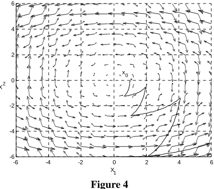
is unbounded for a periodic switching sequence with Z2i =A1, Z2i+1=A2,
i={0,…,m}, and ti =0.5. This is depicted in Figure 4.
-6 -4 -2 0 2 4 6
-6 -4 -2 0 2 4 6
X1 X2
[image:5.595.212.423.452.639.2]* x0
Figure 4
It is clear from the above example that instability may arise in switched linear systems, even if the switching occurs between systems that are themselves exponentially stable. Instability arises in such systems due to the fact that the instability mechanism depends not only on the eigenvalues but also
upon the eigenvectors of the constituent matrices, as well as the choice of switching signal ρ .
stability in an abstract sense, meaning where appropriate, uniform (with respect to initial condition)
global exponential or asymptotic stability.
(i) Arbitrary switching
In many engineering problems, restrictions on the switching signal cannot be specified a-priori. For
such applications, the problem of stability is to obtain verifiable conditions on the matrices (Ai,Bi) that
guarantee the asymptotic stability of the switching system (1) for any switching signal ρ . Clearly,
for this problem to be solvable the system must be asymptotically stable for constant switching sequences, and thus each of the constituent systems must be asymptotically stable. Much of the recent work on the stability of switched linear systems has focussed on this problem; see (Curran 98, Shorten and Narendra, 1998b, Liberzon and Morse, 1999; DeCarlo et al, 2000; Shorten er al., 2002b) for an overview of work completed in this area. Typically, the approach taken here is to develop design laws that guarantee the existence of a Lyapunov function, not necessarily quadratic, that is common to all of the constituent systems. Consequently, much of the work carried out in this area has focussed on developing existence laws (or algorithms) for certain types of Lyapunov function (Narendra and Balakrishnan, 1994a; Mori et al. 1997, Liberzon et. al. 1998; Shorten and Narendra, 1998a, Shorten and Narendra, ).
(ii) The dwell-time problem
Even if the switching system (1) fails to be stable for all possible switching sequences, there may be many practically useful sequences for which it is asymptotically stable. The dwell-time problem is to
explicitly determine a minimum time between switches, min
, such that stability is maintained. More generally we are interested in determining all switching signals that result in instability for the system.
Example 2: Consider the time-varying system given by the following scalar differential equation
0 y t g 5 0 1 y 2 0
y + . +( − . ( )) = , (4)
where y(t) is a scalar function of t, and g(t) is some scalar periodic signal that takes the value -1 or 1. This system can be represented in state space form,
x ) t ( A x
: =
where x=[y,y ], A(t) {A ,A }
2 1
∈ , with
− − =
− − =
2 0 5 1
1 0 2
0 5 0
1 0
2 1
. . A
, . .
A ,
As in example (1), the system Ωcan be thought of as being constructed by switching between the
vector fields associated with the linear time invariant (LTI) systems,
x A x
: i
i =
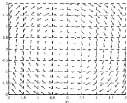
with the Ai defined above. The vector fields associated with each constituent system are depicted in
-2 -1.5 -1 -0.5 0 0.5 1 1.5 2 -2 -1.5 -1 -0.5 0 0.5 1 1.5 2 X1 X 2
(a) The vector field Σ .
-2 -1.5 -1 -0.5 0 0.5 1 1.5 2
-2 -1.5 -1 -0.5 0 0.5 1 1.5 2 X1 X 2
[image:7.595.340.469.109.214.2](b) The vector field Σ .
Figure 5: The vector fields 1
and Σ .
In this example, the form of Equation (4) admits approximate analysis along the lines of describing function techniques presented in (Khalil, 92)
. ( ) .
( cos( ) . . . )
y y f t y
y y f f t h o t y
+ + =
+ + + + + =
0 2 0
0 2 0 1
ω
0φ
0where ,
T
2
0 = T is the period of f(t), and where f + f cos( t+ )+h.ot..
0 1
0 is the Fourier series
representation of f(t). If we assume that the system has a low-pass characteristic, then we may
approximate the system f(t)≈f +f cos(ωt+φ). Hence,
+ + + + = = − + + = − − − + + + + − .
( cos( ))
( )
( . ) ( ( ( ( )) ( ( ( )))
y y f f t y
Y j f
s s f Y j Y j
s j
0 2 0
2 0 2
0 1 1 2 0 0 0
ω φ
ω
ω ω
φ θ ω
ω ω
φ
θ ω
ω
(5)
Now consider the existence of a solution of the form cos( t ( ))
2 2 2 0 0 + +
where
ω
θ is the
phase response of the transfer function at ω . If we again assume a low-pass system characteristic, the
equation (5) yields:
) ) ( t cos( ) f s . s ( f ) ) ( t cos( j s 2 2 2 2 0 2 2 2 2 0 0 0 2 1 0
0 + +
+ + − = + + =
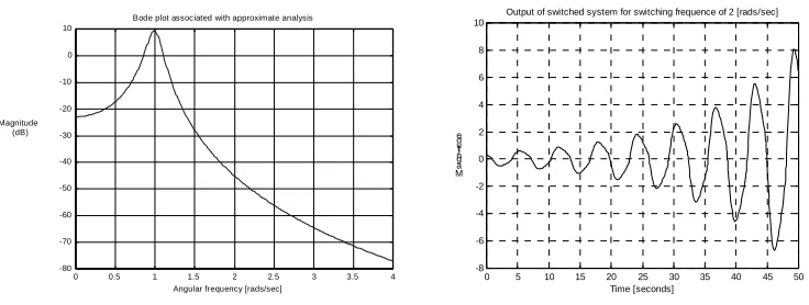
Clearly, the above equation predicts instability everywhere the magnitude of Bode plot of the transfer function
H s f
s s f
( )
( . )
= −
+ 1 +
2
0
2 0 2
0 0.5 1 1.5 2 2.5 3 3.5 4 -80
-70 -60 -50 -40 -30 -20 -10 0 10
Angular frequency [rads/sec] Magnitude
(dB)
Bode plot associated with approximate analysis
0 5 10 15 20 25 30 35 40 45 50 -8
-6 -4 -2 0 2 4 6 8 10
M a g nit u d e
Time [seconds]
[image:8.595.96.464.104.243.2]Output of switched system for switching frequence of 2 [rads/sec]
Figure 6: Response of system
Clearly, instability is predicted for a range of switching frequencies.
The above example is extremely interesting as it indicated the existence of a band of unstable switching sequences, sandwiched between, bands of stable switching sequences. While the above analysis technique provides a reliable method for the determination of this band of frequencies, techniques for analysing general MIMO switching systems are not available. Note also that the instability mechanism in Example 2 differs qualitatively from the instability mechanism in Example 1. In Example 1, instability is induced via unstable chattering, whereas in Example 2 instability is induced via spirals of increasing amplitude. Qualitatively speaking, the system in Example 1 becomes more unstable the faster one switches, whereas the system in Example 2 is unstable for a selective set of switching signals.
(iii) Routes to instability
Examples (1) and (2) illustrate two possible instability mechanisms in switching systems. An open question in the study of switching systems concerns the possible routes to instability. While early work by (Pyatnitski and Rappaport, 1992) and his co-workers on SISO systems suggests that the boundary of stability may be characterised by the existence of marginally stable periodic switching signal, more recent work (Blondel, 2000) suggests that this is, in general, not true. It is therefore of interest to identify particular instability mechanisms for a given switching system. Examples of instability mechanisms include: periodic chattering (Example 1); and periodic spiraling (Example 2). Knowledge of the instability mechanism for a class of system allows one to design non-conservative stability criteria. Hence, problem (iii) is to describe and classify these mechanisms. Initial results in this direction, and in the derivation of non-conservative stability criteria, are reported in (Shorten et al. 2000b, Wulff et. al, 2002).
(iv) Robustness of stability criteria
The concept of robustness with respect to parameter variations is well defined for LTI systems. This issue is somewhat more difficult to quantify for switched linear systems. In particular, robustness may be defined with respect to a number of design parameters, including, not only the parameters of the
closed loop system matrices, but also with respect to switching signal
ρ .
Example 3:
Consider the following system
x(t0) x0, ,
x ) t ( A
where n
R ) t (
x ∈ and where matrices A(t) is constructed by switching between a set of matrices;
, R A }, A , A { ) t (
A i 22
2 1
×
∈
∈ and where
= − − = − − = − 1 L 1 L 1 1 L 1 0 0 K L 1 0 0 K 2 2 M , M M A , A 1 2 1 ,
where K,L>0. The existence of a common quadratic Lyapunov function for the constituent systems Σ
and Σ is a sufficient condition for asymptotic stability of the switching system for arbitrary ρ . A
sufficient condition for the existence of such a function is that the matrices A1 and A2 are Hurwitz, and
that a linear transformation T exists such that TA1T-1 and TA2T-1 are upper triangular matrices (Mori
et. al, 1997, Shorten and Narendra 1998a).
) 0 , 1 ( ) 1 , 0 ( ) 1 , 1 ( L ) 1 , 1 (
L Eigenvectors of A2
Eigenvectors of A1
Clearly, the matrices A1,A2 and M the following properties:
I L lim c) L im l L lim (b) s. eigenvalue identical have and (a) L L L = = ∞ → ∞ → ∞ → ) ( M ( ) ( A ) ( A A A 2 1 2 1
Hence, the matrices A1,A2, can be made arbitrarily close to one another, while at the same time
remaining Hurwitz-stable. In view of the above properties it would not be unreasonable to expect that
the above switching system is asymptotically stable for L large enough. However, it is shown in
(Shorten et. al, 2000) that given any L>1, there always exists a positive K such that an unstable
switching sequence exists for the switching system. Hence, while the existence of a quadratic Lyapunov function for an LTI system provived a quantifiable degree of robustness, arbitrarily small perturbations on the parameters of a switching system can destroy not only the existence of such a function, but also the stability of the underlying switching system.
(v) Numerical approaches to stability: A cautionary word
As mentioned earlier, the existence of a common quadratic Lyapunov function for each of the constituent systems of a switched linear system is sufficient to guarantee the asymptotic stability of the overall system for arbitrary switching signals. The problem of determining whether or not such a
function exists can readily be formulated as a feasibility problem for a system of linear matrix
inequalities or LMIs (Boyd et al, 1994). Recent increases in computational power together with the
any of a number of available software packages. We shall discuss the application of some these techniques to the benchmark example in section 5.2.
Remark
While the numerical methods based on LMIs can be used effectively to establish the stability of a large class of systems, it is important to point out some drawbacks of the approach. First of all, the system parameters must be estimated or known before performing the numerical test for stability. Thus, while LMIs can be used to test a system for stability, they do not provide usable design laws that guarantee stability.
More significantly, the numerical approach can fail to give the correct answer in some cases even for classes of systems for which theoretical results are well established. For an example of this phenomenon, see the stability analysis of the benchmark example in section 5.2.
To further illustrate the point, we present the following example.
Example 4:
Consider the following system
x(t0) x0, ,
x ) t ( A
x= =
where n
R ) t (
x ∈ and where matrices A(t) are constructed by switching between a set of matrices;
, R A }, A , A { ) t (
A i
2 2 2
1
×
∈
∈ with
Now it is well known that when the system matrices of the constituent systems are Hurwitz-stable and upper triangular, the switching system possesses a common quadratic Lyapunov function. However, in this case the MATLAB LMI toolbox fails to find a common quadratic Lyapunov function for the system. (NOTE: This example is of course contrived and is included primarily to illustrate the above point. For a more realistic example see the analysis in section 5.2.)
3.2 Controller realisation and transient response
The issue of transient response is perhaps, from the viewpoint of practical design, as important as the issue of closed loop stability. Clearly, the presence of a switching element as part of a feedback loop is likely to cause transients. Roughly speaking, the transient response properties of the feedback loop are
determined by the eigenvectors, and the eigenvalues, of the closed loop feedback matrices (
and
in Equations (1) and (2) respectively). A comprehensive discussion of shaping the transient response properties of a switched linear system is beyond the scope of this paper; see (Shorten & Narendra, 1998b) for a discussion of the issues involved. Fortunately, several degrees of freedom exist that allow us to manipulate the transient properties of the closed loop system. Here we illustrate, by means of a simple example, several degrees of freedom in the controller realisation that can be manipulated to influence not only the stability properties of the closed loop, but also the transient response properties. In particular, we consider whether the control system should be implemented as a global state controller, or as a local state controller, or as a mixture of both global and local states. The important related issues of state initialisation and the position of the switches in the feedback loop are not discussed due to space limitations.
− −
= −20
1
10 0
1 1
A
− −
= −20
2
10 0
0000001 .
Example 4: Consider the following first order time-varying plant
u K y a
y+ i = pi ,
where y and u are scalars and where ai∈{a1,a2}, Kpi∈{Kp1,Kp2}. Further, we make the unrealistic
assumption that the exact instant at which the plant parameters switch is known, and that this information can be instantaneously utilised to switch the controller parameters. We adopt a pole placement design, and our design objective is to place the poles of the closed loop system at fixed
locations (independent of switching signal),
λ λ
λ , while maintaining unity gain between the
command input and output. We consider a controller structure of the following form,
) b s ( K s K s ) s ( C i i i + +
=1 1 2
and we investigate three implementations of this control structure; a global state approach; a local state approach; and a factored local state approach (both global and local states). In each case we assume a constant input of unity.
(i) Global state controller
In this case the control system can be written,
c i i i i u G r y r e e K e K u b u = − = + =
+ 1 2
where uc is the scalar command signal, and where bi ∈R ,Ki ,Ki ,G∈R.
+
0
1 . By choosing the state
vector as x T
y u
u, , ]
[
= , the following state space representation of the closed loop system is
obtained, r ) t ( B x ) t ( A
x = +
where r=[ uc],A(t)∈{A1,A2},B(t)∈{B1,B2}, and where
= − − = 0 0 G K a K 0 0 0 1 -K a K K K
b 21 i
i pi 2i i i 1 i 1 pi i i
i , B
A ,
and uc=1.
(ii) Local state controller
In this case the controllers take the form
with e defined above. A supervisor switches between the local state controller outputs according to 2
1 (1 (t))u u ) t ( ) t (
u = + − where the signal (t)
takes the value 0 when controller 2 is active, and the value 1 when controller 1 is active.
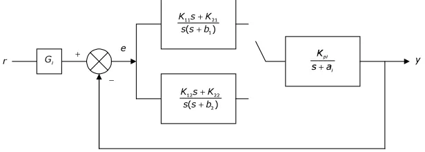
[image:12.595.153.461.157.267.2]+ + + + + − +
Figure 8: Schematic of local state controller for fixed value of t.
With the state vector defined T
] y , u , u , u , u [
x 1 1 2 2
= the corresponding state space equation can be
written, r ) t ( B x ) t ( A
x = +
where r=[ uc],A(t)∈{A1,A2},B(t)∈{B1,B2},
. B , )) ( ( ) ( )) ( ( ) ( )) ( ( ) ( A i i ! " = ! " − − − − − − − − − − = 0 G K 0 G K 0 a 0 K t # 1 0 K t # K a K b K K t # 1 0 K K t # 0 1 0 0 0 K a K 0 K K t # 1 b K K t # 0 0 0 1 0 1 21 1 21 i pi pi 22 i 12 2 2 p 21 pi 21 21 i 11 2 p 11 1 pi 11
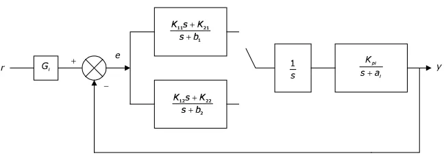
(iii) Factored local state approach (global and local controller states):
Both controllers exhibit integral action. Hence, it is possible to factor the integrator out of both
controllers and include it to, algebraically, as part of the plant. In this case the controllers and the
augmented plant take the form
e K e K u b u e K e K u b u u K y a
y i pi
22 12 2 2 2 21 11 1 1 1 − − = + − − = + = + $ $ $ $ $ $ $
with e defined as before. A supervisor switches between the local state controller outputs according to
2 1 1 % % (t)u ( (t))u
) t (
+ + + + + − +
Figure 9: Schematic of factored implementation for fixed value of t.
With the state vector defined T
] y , y , u , u [ x 2 1
= the corresponding state space equation can be written,
, B , )) ( ( ) (
Ai i
= − − − − − − − − = 0 0 G K G K 0 1 0 0 0 a K t 1 K t K K b 0 K K 0 b 21 21 i pi pi 22 12 2 12 11 1
We note that the parameters of the controllers are identical. Cases (i)-(iii) differ only in implementation. We present one comparative example with the closed loop poles located at
[-0.2,-1.2,-5]. The controller parameters for the example is given in Tables 1.
i ai Kpi bi K1i K2i Gi
1 2 0.1 4.4 -15.6 12 1
[image:13.595.191.425.277.334.2]2 0.25 10 6.15 0.570 0.12 1
Table 1: Plant and controller parameters
0 10 20 30 40 50 60
-200 0 200 400 Ou t p u t
Global state implementation
0 10 20 30 40 50 60
-1 0 1x 10
5
Ou t p ut
Local state implementation
0 10 20 30 40 50 60
0 0.5 1 Time [s] Ou t p ut Factored implementation
(a) Periodic switching between controllers every 10 seconds with a duty cycle of 0.5.
0 10 20 30 40 50 60
-1 0 1 2x 10
41
Ou t p ut
Global state implementation
0 10 20 30 40 50 60
-2 0 2x 10
11
Ou t p ut
Local state implementation
0 10 20 30 40 50 60
0 0.5 1 Time [s] Ou t p u t Factored implementation
(b) Periodic switching beween controllers every 1 seconds with a duty cycle of 0.5.
Figure 10: Response to unity input of various realisations
It is clear from the above plots that the qualitative response of each implementation is very different. For both switching sequences, the response of the local state and the global state controllers is unsatisfactory; in (b) the global state controller is unstable. This is a genuine switching instability;
namely, both A1 and A2 are Hurwitz-stable, but as a result of switching instability occurs. The local
[image:13.595.168.444.404.444.2]from the output of the feedback loop; see work in (Shorten and O’Cairbre, 2002) for initial stability results for local state controllers.
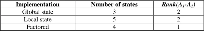
Remark: Global state, local state and factored implementations, and a new problem in switching
The fact that controller realisation can have such an impact on the performance of the closed loop system has profound implications for control design. An important question is to account for and exploit these differences for the design of control systems. Clearly, whenever all controllers share the same structure then the controller may be implemented in the form of a parameter varying system (state sharing), or by switching between the individual controllers (local state), and sometimes in the form of a factored implementation. In the global state case the controller has a single state, where as in the latter cases each of the controllers have local states. An obvious difference between the two cases is that the global state approach results in a control output that is continuous at the switching instants, whereas the local state approach results in a controller output that is discontinuous at the switching instants. Other differences between the two approaches is that the global state approach requires fewer states to implement, and that the global state approach results in a controller structure that is itself parameter varying and hence can be potentially destabilised by means of switching. In the above example, the controller parameters are identical in both cases and are given in table 1. However, the state space realisations are quite different. The local state implementation results in a closed loop system that has a higher order than that of the global state implementation or of the factored state implementation.
Implementation Number of states Rank(A1-A2)
Global state 3 2
Local state 5 2
[image:14.595.133.462.365.416.2]Factored 4 1
Table 2
A more crucial observation concerns the rank of the matrix (A1-A2); instability mechanisms for global
state control system are excited via rank-2 perturbations, whereas instability in the factored implementation is excited via a rank-1 perturbation. While it is true to say that few stability results are known that are valid for rank-2 perturbed systems, the rank-1 case is well understood. In fact, it is shown in (Shorten and O’Cairbre, 2002) that system matrices that share n-1 common eigenvalues, and
which satisfy rank(A1-A2)=1 result in asymptotically stable switching systems.
Example 4 illustrates another very important characteristic of the factored implementation; namely that the switching action is completely unobservable from the output of the control system. We note that it is impossible to realise such a design specification with the global state implementation (without state re-initialisation), or with the local state controllers (with unstable local controllers). The poor performance of the control structure is due to the fact that after switching the controller must find its equilibrium condition under the dynamics of the closed loop. Such effects can be avoided by employing local state controllers (with stable controllers). In this case the new equilibrium condition can be found by switching between the controller outputs. A simple condition for unobservability of the switching action, for a constant command input, is that the steady state gain between the command and the output is constant. While it is relatively easy to design local state controllers (where the controllers are stable) to achieve this property for constant input signals (Shorten 96), the question of whether or not this is possible for arbitrary input signals has not yet been explored. It is therefore of interest to pose the following question:
Observability of switching action: Given a class of input signals ∈ϑ, for what class of switching systems,
C(t)x, y
0 0
=
= +
=A(t)x B(t)u, x(t ) x , x
:
4. A Benchmark System
In many control applications, the controller includes switches and its performance depends directly on the successful resolution of the issues discussed above. Indeed, these aspects of the controller design may be the most important. One such application is the control of large-scale grid-connected variable-speed pitch-regulated wind turbines. The wind turbine system essentially consists of a rotor, a low-speed shaft, a gearbox, a high-low-speed shaft and a generator. The rotor blades pitch about their longitudinal axis. A much-simplified representation of the dynamics of a 1MW three-bladed machine is proposed as a benchmark switched system. A block diagram representation of this system is depicted in Figure 11. The characteristics of the turbine component sub-systems and specification of the control design task are described below (see Leithead & Connor 2000a and references therein for detailed, generic derivation and validation of a more complete description).
4.1 Plant dynamics
(i) Power train
The combined dynamics of the drive-train and generator are essentially linear and, together, are modelled by
xp =A xp p+B Tp (6)
with x T A B p p p = = = − − ′ − ′ − − + ′− ′
L
N
M
M
M
O
Q
P
P
P
= −L
N
M
M
M
O
Q
P
P
P
ΩLD LS ΩLS T
LD rtr T
T T T
I NI
K N K
N K N K I I K N K I
I I , / / / / / ( ) / / / ( ) / , / / γ
γ γ γ γ γ
2 2 2
1 1
1 3
2 1 1 1 1
2 2 1 2 1 1 0 0 1 1 0 0 0 0 1
d
i
d
i
(7)
where TLS is the torque on the low speed shaft, ΩLS is the speed of the low-speed shaft, ΩHS is the
speed of the high-speed shaft, ΩLD is the generator speed, Trtr is the torque generated by the rotor, TLD
is the generator reaction torque (set via power electronics). The parameter values are N=58;
I1=1.0295×10⁶; I2=42.82; K1=1.0106×10⁸; K2=4.85×10⁶; γ1=1.5176×10⁴; γ2=4.5112; γ′= 2.6538×10⁵,
/
K K K
K N 1 1 1 2 2 1
=
F
+HG
I
KJ
. (It should be noted that the value of γ1 embodies the linear component of thedamping introduced by aerodynamic effects). The transfer function relationship, equivalent to (6), is
ΩLD
LD rtr
s s s T s T s
s s s
( ) . . . ( ) . ( )
. . .
=− + + +
+ + +
0 02335 0 00633 2 279 0 0393
0 3764 794 9 20 57
2
3 2
c
h
(8)(ii) Pitch actuator
The pitch actuator position is physically constrained to be greater than or equal to zero degrees. The actuator dynamics may be neglected for analysis purposes. For completeness, however, it is noted that these are
,
xz =A xa a +Bap p =C xa a (9)
Aa Ba C
p = − − −
L
N
M
M
M
O
Q
P
P
P
=L
N
M
M
M
O
Q
P
P
P
0 1 0
526 62 28 57 1022 73
0 0 0 1022 73 0 . . . ( ) , . , ν
a= 0 0 1 (10)
where p and
p are, respectively, the actual and demanded blade pitch angles and ν(
) p p p = > ≤
R
S
T
1 0 0 0(iii) Aerodynamics
By suitably augmenting the plant (see Appendix), the aerodynamic torque, Trtr, generated by the
rotor may be approximately modelled by
Trtr= KVV2 - Kp ∆(p, ΩLS) p (11)
where V is the effective wind speed, see below, and ∆(p, ΩLS) is an unknown gain (representing
uncertainty in the aerodynamic characteristics) with nominal value of unity, Kp=29500.0 and
KV=3200.0.
(iv)Wind disturbance
The rotor interacts with a complex spatially and temporally varying field. However, the wind-field may be represented by a single wind speed constant over the rotor disk, the effective wind speed. It should be noted that the spectral characteristic of this effective wind speed is very different from
that of a point wind speed. For a given mean wind speeds Vmean, a suitable model for the effective
wind speed is the linear stochastic equation
(
)
(
)
,
int int int
V
a
a
a V
V
a
a
b V
V
a
a
pox
x
w mean po
x
x
w mean po
x
x
1 2
1 2
1 2
0
0
0
1
1
0
0
0 1 0
12 3
2 3 1 2 3
2 2
3 2
2 3
2 3
2 3
L
N
M
M
M
O
Q
P
P
P
=
−
−
+
−
−
+
L
N
M
M
M
M
M
M
M
O
Q
P
P
P
P
P
P
P
L
N
M
M
M
O
Q
P
P
P
+
L
N
M
M
M
O
Q
P
P
P
=
L
N
M
M
M
O
Q
P
P
P
τ
τ τ
τ τ τ τ τ
τ τ
τ τ
τ τ
τ τ
η
b
g
b
g
V
(12)where
τ
1=
β
/
2
,
τ
2=
τ
1a
,
τ
3=
β
/
a
,β =
33 8
. /
V
mean,
a
=
0 55
.
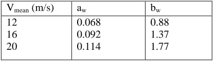
and η is Gaussian white noisewith zero mean and unity variance. Suitable values for aw and bw (capturing the dependence on the
mean wind speed of the spectral characteristics of the effective wind speed) are given in Table 3,
Vmean (m/s) aw bw
12 16 20
0.068 0.092 0.114
[image:16.595.203.412.458.518.2]0.88 1.37 1.77
Table 3 Mean wind speed dependent parameters for wind disturbance model.
4.2. Design task: control requirements
The overall objective of the controller is to maximise energy production, whilst working within actuator operational limits and minimising the extreme loads and associated fatigue damage on the turbine structure and drive train. This is a disturbance rejection task.
(i) Measured variables
Measurements are available of (i) the instantaneous power P (i.e. the product TLDΩLD) and (ii) the
generator speed ΩLD. The sensor dynamics can be assumed negligible, as is measurement noise. Note
that the effective wind speed, V, cannot be measured.
(ii) Manipulated variables
The controller is able to adjust (i) the blade pitch angle and (ii) the generator reaction torque, TLD.
(iii) Physical constraints
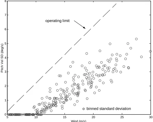
deviation of the rate of change of the pitch angle reflects the actuator activity over the medium and long term and is required to remain less than (0.4V-1.8) deg/s over the operating range of mean wind speeds up to 24 m/s (the dependence of the bound on wind speed is associated with the augmentation of the plant to compensate for the aerodynamic nonlinearity – see Appendix). Secondly, in order to avoid exciting structural resonances and to remain within design loadings, the turbine is not to be continuously operated (i.e. in steady state) at rotor speeds above 2.72 rads/sec. Of course, fluctuations in the mean wind speed induce transients (about the steady state operating point) in the rotor speed. These transients must remain strictly less than 3.264 rads/sec under the normal range of operating
conditions. The former limit is denoted
Ω
LSmaxcontand the latterΩ
LSmax. The generator reaction torque,TLD, must be positive (to avoid "motoring") and the generator is not to be operated continuously (i.e. in
steady state) above a level, Prated, of 1MW.
(iv) Robustness
The uncertainty in the plant dynamics is primarily associated with the rotor aerodynamics. In addition to the use of a relatively crude aerodynamic model for control design purposes, the rotor aerodynamics typically exhibit considerable variation during normal operation (associated with, in particular, the accumulation of environmental deposits on the blade surfaces). The closed-loop system is therefore
required to remain stable for arbitrary time variations in the uncertain gain ∆ in the interval [0.5,2].
(v) Operational Requirement
The overall objective of the controller is to maximise energy production, whilst working within the operational limits of the turbine, and minimising the peak loadings experienced. While the wind is highly stochastic, initial insight into this requirement can be gained by considering the situation when the wind is steady and the turbine is in equilibrium. Three operating modes can be identified.
1. Energy capture limited by available wind energy 2. Energy capture limited by rotor speed constraints 3. Energy capture limited by generator rating
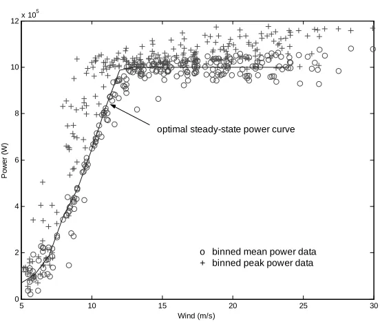
(vi) Performance assessment
Performance is measured as follows (the approach adopted is semi-empirical in view of the complex, stochastic nature of the wind disturbance; see Leithead & Connor 2000b). Time histories of the controlled system are collected for turbulent wind conditions with mean wind speeds
Vmean∈{5,8,10,12,14,16,18,20,22} m/s. The time histories are each of 600 seconds duration (after
discarding the initial 20 seconds to allow the system to settle down) and are partitioned into 10 second intervals. The short-term mean wind speed, mean power, mean generator torque, peak power, maximum rotor speed, minimum generator torque and standard deviation of pitch actuator velocity are determined for each interval. This interval data is sorted into 1 m/s wide bins according to the
short-term mean wind speed. Let Vi denote the centre wind speed of the i
th
bin. The average of the mean
power data in the ith bin is a measure of energy capture at wind speed Vi . Let µi denote the average of
the peak power data in the ith bin. Then µi is a measure of the peak load experienced by the wind
turbine at wind speed Vi. Energy capture is to be maximised and peak loads minimised, subject to
operating constraints. Note that a high penalty is placed on peak loads during above rated operation
as these are related to fatique and therefore the impact is dominated by the peak values. A penalty is placed on sub-optimal energy capture during below rated operation as in practice this would lead to
operation in the aerodynamic stall regime (not modelled here). Similar calculations for the maximum
rotor speed data, minimum generator torque data and pitch actuator velocity data provides,
respectively, an upper bound on ΩLS (required to be less than ΩLS
max
), a lower bound on TLD (required
to be positive) and an upper bound on pitch actuator velocity. A further, deterministic, extreme gust is employed to confirm the ability of the controller to maintain operation within the allowed rotor speed limits. This gust is a pulse with an initial wind speed of 22 m/s, falling to 12 m/s over 10 seconds and then returning to 22 m/s.
4.3 Discussion
switching action. Additionally, the changes between the three modes of control operation require switches. These switches are activated very frequently and randomly by the stochastic variation in wind speed. Nevertheless, the robust stability of the controlled system must be maintained. Furthermore, the transients associated with the switches can very easily cause the performance requirements to be breeched. Hence, suppression, indeed elimination, of the switching transients is critical. In contrast to the examples in Section 2, which are not untypical of those considered elsewhere in the literature, the wind turbine system, having multiple switches and higher order dynamics, is rather more complex as indeed are many switched systems in practice.
5 Baseline Design: Classical Controller
Successful solutions to the pitch-regulated variable speed wind turbine control design task are known and are described in Connor and Leithead (1996). A similar controller for the wind turbine system presented above is described in this section.
5.1 Baseline controller
Clearly, the performance requirements cannot be met with a single linear controller. Reflecting the natural division of the turbine operation into separate modes, the approach standard in commercial practice is adapted whereby in each mode of operation a particular control action is chosen and an individual controller is designed. Subsequently, the individual controllers are integrated to obtain a full envelope controller.
(i) Operating mode 1
The controller is configured to regulate rotor speed to maximise energy capture by adjusting the generator reaction torque whilst maintaining the blade pitch angle at zero. Under nominal steady state
conditions, the maximum power is generated when TLD =K VV 2/2N
. Unfortunately, as the
effective wind speed V is not measurable, direct regulation of TLD to meet this equality is impossible.
Instead, an indirect approach must be used. In steady conditions generating maximum power, the
generator speed is
Ω
LD=
NK V
V 2/ (
2
γ
1+
N
2γ
2)
. That is,K V
v 2=
2
(
γ
1+
N
2γ Ω
2)
LD/
N
.Consider, therefore, the control law
T C N
N
LD= LD LD
+
(
γ
1 2γ
2)2 Ω (13)
where
CLD =
+
1
0 05. s 1 (14)
provides additional roll-off to suppress the resonance in the turbine drive-train. (Note that in actual
wind turbine controllers it is more usual to select TLD proportional to ΩLD2 rather than ΩLD. The linear
law used here approximates the usual quadratic law, in accordance with the simplified aerodynamic model used).
(ii) Operating mode 2
The controller is configured to regulate rotor speed, ΩLSmaxcont, at a constant value by adjusting the
generator reaction torque while maintaining the blade pitch angle at zero. Using classical loop-shaping techniques, the controller transfer function is designed to incorporate integral action to ensure rejection of changes in mean wind speed. The controller designed is
T C N C N
N
LD LS
cont
LD LD LD
= 1 − + +
1 2
2 2
Ωmax Ω ( )Ω
c
h
γ
γ
(15)C s
s s s s
1 2
5 1
4 14 0 05 1
= +
+ + +
1200( )
( )( . ) (16)
Observe that, with the aim of simplifying the overall design, the mode 2 controller (15) is obtained by suitably augmenting the existing mode 1 controller, (13). The gain margin is 9.67 dB, the phase
margin is 56.51° and the cross-over frequency is 1.30 rad/s.
(iii) Operating mode 3
The controller is configured to regulate rotor speed at a constant value, ΩLSmaxcont, by adjusting the
blade pitch angle whilst keeping a fixed generator reaction torque, Tref. Neglecting, for the moment,
the high frequency drive-train resonance, the plant dynamics (6) may be simplified to
ΩLD Ω Ω
rtr LD LD p LD LD V
NT N T
I
NK p N T I
NK
I V
= − 2 − 1 =− − − +
1
2 1
1 1
2
γ γ
(17)
Evidently, the aerodynamic torque and generator torque are matched in the sense that they enter the equation in the same manner, albeit with a gain difference of N. Hence, despite the physical structure of the system being quite different in modes 2 and 3 (in mode 2 control action applied via the generator torque alone, while in mode 3 the system is configured as MIMO with control action applied via both the pitch angle and generator torque), in terms of the plant dynamic characteristics these modes are closely related.
Using classical loop-shaping techniques, the controller is designed as
( )
max
p N
K C N
N N
p
LS cont
LD LD
= 2 − + +
1 2
2 2
Ω Ω Ω
c
h
γ γ (18)where C2 denotes linear dynamics with transfer function
C s
s s s
2 2
5 1
4 14
= +
+ +
1200( )
( ) (19)
Observe that, at least at low frequencies, the controller transfer function is closely related to that employed in mode 2, reflecting the similarity in plant dynamics in modes 2 and 3 noted previously.
The gain margin is 9.84 dB, the phase margin is 59.63° and the cross-over frequency is 1.33 rad/s.
(iv) Full envelope controller
It remains to integrate the separate mode 1, 2 and 3 controllers to produce a full-envelope controller implementation. Firstly, it is noted that the mode 2 and 3 controllers are designed to directly augment the mode 1 controller, thereby simplifying implementation. Secondly, the mode 2 and 3 controllers possess similar low frequency dynamics. The latter can be made explicit by partitioning the mode 2 and 3 controller transfer functions as
C1=CLDClow , C2=Clow (20)
where
C s
s s s s
low =
+
+ + = +
1200
CLD
( )
( ), .
5 1
4 14
1
0 05 1
2
b
g
(21)During mode 1 operation, the integrator in Clow can "wind up" resulting in excessive transients
following a transition from mode 1 to mode 2 operation. Transients may also be associated with the
other low frequency dynamics elements of Clow. Following Leith & Leithead (1997), and similarly to
a number of popular anti-wind up approaches, this issue is addressed here by partitioning Clow as
C s
s s s
i = -15.625
( )
( )
5 1
4 14
2
+
+ + , Co =76 8. (22)
and enclosing the dynamics Ci within a minor feedback loop during mode 1 operation. The
partitioning into Co and Ci is selected such that the bandwidth of the minor loop is similar to that of the
closed-loop system during mode 2/3 operation. Switching from mode 2 to mode 3 operation is based on the generator reaction torque. The resulting full envelope controller implementation is shown in Figure 12. Observe that the switches within the controller are formulated as continuous (but non-differentiable) nonlinear functions of the switch input. Hence, the admissible switching sequences are
immediately evident from the block diagram. The constant Tref is defined by
Tref = Prated/NΩLS cont
max
(23)
that is, Tref is the generator torque at which rated power is developed when operating at rated speed.
This is used within the controller in a straightforward manner as a threshold on internal signals to determine the required mode of operation.
Remark: The following state-space realisations are employed.
CLD: xLD =ALDxLD+BLDT1 , TLD =C xLD LD (24)
CiCo:
,
max
xlow A xlow low Blow LS C x cont
LD B To low low
= +
d
c
NΩ −Ωh
+ 1i
T2=where
A B
C D
A B
C D l B
LD LD LD LD
low low low low
o
L
N
M
O
Q
P
=L
−N
M
O
Q
P
L
N
M
O
Q
P
=− − −
L
N
M
M
M
M
O
Q
P
P
P
P
= 20 4
5 0
40 35 0
40 0 0
25 0 25 0 3125
0
0
0 0 1 0
00130 ,
. .
.
. .
.
, .
(25)
(v) Performance
Many different ways of integrating the individual controllers for the separate modes is possible but it is emphasised that the performance is sensitive to the way in which this integration is achieved. The particular full-envelope controller described above achieves good performance and fully meets the performance specification. Although its performance can be improved upon, the required modifications increase its complexity. Hence, to facilitate analysis, this baseline controller represents a suitable compromise between performance and complexity. Detailed performance plots are shown in
Figure 13. A Simulink model of the plant and controller is available at www.hamilton.may.ie,.
5.2 Analysis challenges
The baseline controller design immediately creates a number of analysis tasks. While analysis of the robust stability and performance of the full-envelope closed-loop system is required, the local pair-wise analysis of the operating modes nominal stability presents a task of sufficient difficulty for present purposes. While reading this section, it is important to keep in mind that we are dealing with mode 1/mode 2 switching and mode 2/mode 3 switching separately. We do not consider switching between mode 1 and mode 3.
(i) Stability of mode 1/2 operation
During operation encompassing modes 1 and 2, the closed-loop dynamics (neglecting the additive wind disturbance and the constant reference inputs to the controller) are
&
,
{ ,2}
x x x x A
B C
B C A B C
B C A
A
A B C
B C A
B C B C A
= = − + + = − +
L
N
M
M
M
M
M
O
Q
P
P
P
P
P
L
N
M
M
M
M
M
O
Q
P
P
P
P
P
[ ] , ( ) , ( )p low LD
p p LD
low p low low low
LD p
p p LD
low p low LD p LD low T B N N N N 1 1 0 1 2 2 2 0 2 1 1 2 2 2 0 0 0 0 0 0 A
γ γ γ γ
(27)
where Bp1 denotes the first column of Bp, Cp=[1 0 0] .
One standard approach to stability analysis of a switched system of the form (26) is to search for a
common quadratic Lyapunov function (CQLF), xTPx. That is, for a matrix P such that
P>0, A P1T +PA1<0, A PT2 +PA2 <0 (28)
The existence of such a matrix guarantees the exponential stability of (26) for all switching sequences (e.g. see Liberzon & Morse 1999, Shorten & Narendra 1998b and references therein). As mentioned in section 3, the existence of a CQLF can be established numerically using software for solving LMIs. A
direct search for a matrix P satisfying the inequalities (28) performed using the LMI toolbox in
MATLAB fails to establish the existence of a CQLF for the system (26). In fact, the toolbox finds the system of LMIs (28) to be marginally feasible, meaning that it is unable to find a CQLF while also being unable to definitively rule out the existence of one. However it can be confirmed using the following direct analytic arguments that no CQLF exists for this system. A necessary condition for the existence of a CQLF is that the matrix pencils
1 2 1 2 1 A ) ( A A ) ( A − − + − + 1 1
must be Hurwitz for [ 10,].
∈ (Shorten and Narendra, 1999). This clearly implies that both pencils
must be non-singular for [ 10,].
∈ However, it follows from the fact that the matrix product
2 1A
A has negative real eigenvalues that the pencil 1
2
1 ( )A
A + 1− −
is not Hurwitz for some
]. , [ 10
∈ Thus, the system (26) cannot have a CQLF. For more details on this analysis consult
(Mason, Shorten & Leith, 2001) and the references therein. This is an example of the situation described in section 3, where a numerical approach to stability analysis can fail to provide the correct answer where alternative direct arguments succeed.
While the forgoing analysis considers quadratic Lyapunov functions, LMI based analysis may be extended to encompass searching for the existence of a class of piecewise-quadratic Lyapunov functions (Johansson & Rantzer 1998). The state-space is divided into two regions or cells, with mode
1 effective in cell 1 (x6<0) and mode 2 effective in cell 2 (x6≥0). To establish stability via piecewise
methods, a Lyapunov function of the form
= (29)
is sought, where the matrices Pi are parameterised so as to ensure that the function is continuous across
the boundaries between the cells. Namely, following Johansson & Rantzer (1998) the matrices Pi are
parameterised as Pi=Fi
T
TFi,i=1,2 where the matrix T is to be determined and F1x=F2xon the shared
cell boundary. Note that these matrices are not uniquely determined by the partition. This formulation relaxes the requirement of a common quadratic Lyapunov function in two ways. Firstly, we do not
require a single positive definite matrix P to simultaneously satisfy A P PAi 0
T
i + < for each i.
Secondly, when implementing the search for such a function as a system of LMIs, x A Pi PiAi x
T i T
)
( + is
not required to be negative for all non-zero x but only for those x in the cell i where the dynamics