An Automatic Sequential Recognition Method for
Cortical Auditory Evoked Potentials
Ulrich Hoppe, Member, IEEE, Stephan Weiss*, Member, IEEE, Robert W. Stewart, Member, IEEE, and
Ulrich Eysholdt
Abstract—The detection of cortical auditory evoked potentials
(CAEP), which are part of the electroencephalogram (EEG) in re-action to acoustic stimuli, has important applications such as deter-mining objective audiograms. The detection is usually performed by a human operator, with support from often basic signal pro-cessing methods. This paper presents a novel mechanism for the detection of CAEPs, which is fully automatic and stops the mea-surement when a given confidence is reached. This proposed de-tector comprises of three stages. First, a feature extraction by a wavelet transform parameterizes the time domain EEG signal by only few transform coefficients. This feature vector is then classi-fied by a neural network which yields a binary vote on every EEG segment. Finally, a sequential statistical test is performed on suc-cessive classifications; this stops the measurement if a specified de-cision confidence has been reached. The adjustment of the detector according to a clinical database is discussed. Thus adjusted, the proposed CAEP detection scheme is applied to a study, and com-pared with a human operator. The results demonstrate that this method can attain similar results, but outperforms the human ex-pert for stimulation levels close to the hearing threshold.
Index Terms—Automatic detector, cortical auditory evoked
po-tentials, neural networks, sequential statistical test, wavelet anal-ysis.
I. INTRODUCTION
C
ORTICAL auditory evoked potentials (CAEPs) can be ob-served as part of the electroencephalogram (EEG) and re-flect the neural processing of acoustic stimuli in the cortex. In their clinical application, CAEPs have the advantage of enabling frequency specific testing of the hearing ability by appropriate selection of the stimulus [1]. The recognized presence or ab-sence of a CAEP in response to an acoustic stimulus of speci-fied frequency and level can be used to determine an objective audiogram. Objectivity is achieved in the sense that the active cooperation of an experimentee or patient is replaced by the in-terpretation of the EEG by an operator [1]. Objective hearing as-sessment is important to, for example, establish reliable hearingManuscript received August 27, 1998; revised October 11, 2000. This paper was presented in parts at the 1996 IEEE EMBS conference in Amsterdam, and selected as a finalist paper in the European student paper competition. Asterisk
indicates corresponding author.
U. Hoppe is with the Department of Phoniatrics and Pediatric Audiology, University of Erlangen-Nürnberg, Bohlenplatz 21, D-91054 Erlangen, Germany (e-mail: [email protected]).
*S. Weiss is with the Department of Electronics and Computer Science, Uni-versity of Southampton, SO17 1BJ, U.K.
R. W. Stewart is with the Department of Electronic and Electrical Engi-neering, University of Strathclyde, Glasgow G1 1XW, Scotland, U.K.
U. Eysholdt is with the Department of Phoniatrics and Pediatric Audiology, University of Erlangen-Nürnberg, Bohlenplatz 21, D-91054 Erlangen, Ger-many.
Publisher Item Identifier S 0018-9294(01)00567-5.
thresholds for persons with low compliance, e.g., small children [2]. The work presented here is concerned with an automatic de-tector to help and assist in identifying CAEPs.
When an acoustic stimulus reaches the inner ear it elicits neural activity along the neural auditory pathway from the spiral ganglion via nerve fibers over the brainstem up to the auditory cortex, where it results in auditory perception approximately 100 ms after the onset of the stimulus [3]. Triggered by pro-cessing in the auditory cortex [4], CAEPs, therefore, give evi-dence of correct auditory perception. According to [5] and refer-ences therein, for most human adults the signal properties of the CAEP are quite similar when the same measurement paradigm is used and the central auditory processing is normal. The CAEP consists of waveforms with specific latencies with respect to the stimulus onset. The literature names their minima and maxima
due to polarity and sequence and , whereby
and are the most stable waves of a CAEP with peak la-tencies of about 100 ms and 175 ms, respectively [5]. It is gen-erally the recognition of this - -complex which is used to establish one of two hypotheses : no CAEP within EEG; and
: CAEP within EEG [6].
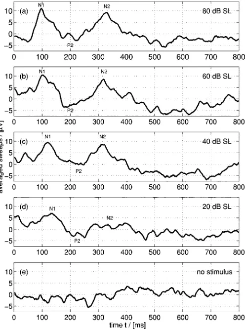
Variations of amplitudes and latencies of the CAEP waves occur and depend—besides age, sex, ear of stimulation, hearing ability, and vigilance of the experimentee—on the frequency, level and repetition rate of the stimuli [5]. While many of these factors only contribute little or can be controlled during the measurement, the individual sensation level is in general unknown and has an observable influence: As the stimulus level approaches the hearing threshold, the CAEP waves appear weaker and more delayed due to prolonged auditory processing for quieter sounds [3]. An example is given in Fig. 1, where averaged EEGs recorded synchronously to stimuli of different intensities are shown.
Besides this variability, detection of CAEPs is impeded by background EEG due to visual, motoric, and sensoric activities of the experimentee, resulting in a very low signal-to-noise ratio (SNR) of less than 10 dB. As CAEP and background EEG cover similar frequency bands, it is impossible to detect a CAEP from EEG measurements with only a single stimulus. Rather, the detection of CAEPs generally has to be based on repeated stimuli and the acquisition of typically about 30 to 80 “sweeps” which, here, refer to EEG segments recorded under identical conditions synchronously to the given stimulus. Many methods for support in this decision have been proposed, and range from simple averaging to more advanced signal processing.
Simple averaging of successive sweeps is a common, but often sub-optimal CAEP reconstruction method, since station-arity of the background noise, invariance of the CAEP, and
Fig. 1. EEG averages over 100 sweeps obtained from a single individual: (a)–(d) variable stimulation intensities of 80, 60, 40, and 20 dB above hearing threshold (SL) applied att = 0 containing CAEP; (e) no stimulation (01 dB) and, hence, no CAEP.
the absence of correlation between CAEP and noise have to be assumed. Due to varying vigilance and habituation effects during the measurement, this is only approximately satisfied [7]. Methods have been proposed to take variations of the background EEG into account by estimating the noise power in every sweep [8]–[11], and weighting their contribution to the average accordingly. Thus, noisier sweeps and artifacts are disemphasized. Other approaches try to enhance the SNR by considering the variations of the central auditory processing during the measurement [12]–[14]. These techniques assume that the latencies of the CAEP vary over time, leading to an approximate affine translation of the signals. The actual translations are estimated by cross correlation of every single sweep with predefined patterns. SNR enhancement is then achieved by averaging the latency-corrected sweeps. Clearly limited by the small sample size for variance-type estimations, such methods can only be moderately successful.
A number of parametric approaches aim to replace the subjec-tive interpretation of the averaged CAEP by an automatic classi-fication, which is generally based on the statistics of some sweep parameters. Literature offers a wide range of parameters being used, like CAEP relevant samples of the digitized signals, se-lected Fourier coefficients, energy of averaged sweeps, or cor-relation coefficients with “normal” CAEP [15]. Coarse SNR es-timates of the CAEP/EEG based on the comparison of a
stan-dard average with a “ average,” where every second sweep is included with reversed sign, were also used to classify CAEPs [16], [17], [15]. Wavelet coefficients have been used to parame-terize evoked potentials successfully [18], and have been shown to perform at least comparable to the above parametric methods for CAEPs [19]. However, such parametric approaches require to
a priori set a threshold for classification and cannot provide
stop-ping criteria for the measurement based on a specified error rate, which usually is regarded as major drawback in clinical use.
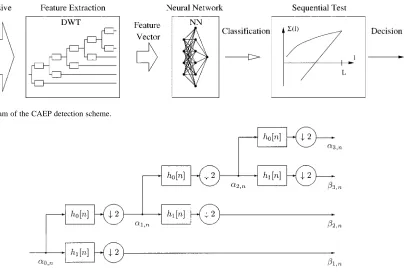
In the approach proposed here, the good parameterization property of the wavelet transform is exploited to build a detector with stopping criterion and specified error rate. This detector is outlined schematically in Fig. 2. First, a selected set of discrete wavelet transform (DWT) coefficients, a so called “feature vector” (FV), is calculated for each measured sweep. The dimen-sion of the FV can be much smaller than the original time-domain signal without loss of too much information on a CAEP [18], [19]. The FVs of successive sweeps are each classified by a neural network (NN), which maps the FV onto a single binary output. A similar approach is implemented by wavelet networks [20], which combine both a wavelet transform for parameterization and an NN in a hybrid classifier. As the binary classification of the NN bears a high type-I-error (incorrect acceptance of ), a sequential statistical test forms the last stage of the detection procedure, judging the number of positive and negative sweep classifications produced by the NN. This test will provide a decision based on a predefined type-I-error rate, and stops the measurement when this confidence limit is reached.
In Section II, the proposed detector is introduced in detail. Section III reports on the EEG equipment at hand and the re-sulting data properties, which are used to adjust the different stages of the detector. This includes the selection of the FV, the dimensioning and training of the NN, and the adjustment of the sequential statistical test. The application of our method to a study using clinical data is reported in Section IV, compared to the results achieved by a human operator. Finally, we draw con-clusions in Section V.
II. AUTOMATICDETECTORMETHODS
This section describes in detail the principles of the proposed detection scheme and its components. The parameterization by DWT coefficients is addressed in Section II-A. Section II-B introduces a NN classification of the features, thus, extracted by the DWT. Finally, a sequential statistical test to assess the classification results of successive sweeps is introduced in Section II-C. The adjustment of the detector components with respect to EEG/CAEP data will be performed in the separate Section III.
A. CAEP Feature Extraction by Wavelet Transform
Fig. 2. Block diagram of the CAEP detection scheme.
Fig. 3. Octave filter bank to compute an MRA of depthD = 3; deeper decompositions are achieved by further splitting .
basis functions, which is advantageous when analyzing transient signals [21]. For the DWT considered here, a set of orthogonal basis functions is obtained by scaling and translation of a mother wavelet.
An efficient calculation of the DWT coefficients in the case of discrete-time data can be achieved with a multiresolution algo-rithm (MRA, [22]). For a dyadic DWT, this MRA is performed by filtering the signal to be analyzed with an octave filter bank as shown in Fig. 3. The high-pass filter forms a quadra-ture mirror filter (QMF) pair [23] with the low-pass of the filter bank. The input sequence to the octave filter bank, , is the signal to be analyzed. Through successive low- and high-pass filtering of the samples in the lower frequency band, , and decimation of the resulting signals by a factor of two (denoted as ), subband samples are obtained, which, except of the lowest frequency band, represent the DWT coeffi-cients. The coefficients are intermediate values and corre-spond to a dual basis function of the wavelet, a so called scaling function [22]. The filters and are sampled version of the underlying scaling function and wavelet and, therefore, deter-mine which DWT—amongst a large variety of possible wavelet functions (see, e.g., [22], [21], and [24])—is being implemented. Since the signal to be analyzed, , is only defined on a fi-nite interval , suitable signal extensions [25] or boundary filters [26] have to be selected. As both yield identical results [26], for ease of implementation the first possibility will be pursued. Zero padding is not viable for decomposition with a deep octave bank, as information will be blurred over large intervals by the transient behavior. Periodization of the original data and all intermediate filtering results however permits to filter in steady-state and, thus, retain all required information within a preserved period of the signal. With the possibilities of odd or even periodization [25], the MRA yields DWT
coeffi-cients that completely describe the original time series com-prising samples. However, restrictions to symmetric wavelets apply, if an odd periodic extension is selected [22].
Based on EEG data, Section III will determine, which wavelet function and periodic extension will be used for the proposed automatic detector and which coefficients can be isolated as sig-nificant. The task will be to identify a subset of coef-ficients collected in a FV, , that can describe the CAEP suf-ficiently well. Section III will also show why these coefficients on their own can only yield a rather unsatisfying indication of a CAEP. This will motivate the requirement of the NN classifi-cation and sequential test performed on the selected significant DWT coefficients in the FV described in Section s II-B and Sec-tion sII-C to ensure a reliable and systematic CAEP detecSec-tion.
B. NN Classification
The aim of this section is to introduce a classification method for single sweeps distinguishing between “containing a CAEP” or “not containing a CAEP” based on the set of DWT coef-ficients in the FV. Due to interindividual variations of CAEP-la-tencies and -amplitudes these FVs do not exhibit a single specific pattern. Instead, many patterns must be regarded as being specific for CAEPs. So far, there exists no theoretical treatment of this dis-crimination problem; hence, heuristic classifiers have to be used. Artificial NNs provide the possibility of learning by groups of sample FVs and require only little computational effort.
A multilayer perceptron was used for classification of the FV calculated for each sweep. This type of NN comprises an input layer with nodes corresponding to the dimension of the FV, one hidden layer with neurons and an output layer with a single
neuron ( network). Since the NN is a nonlinear
-norm are applied to the FV prior to feeding it into the NN. This operation excludes interindividual amplitude differences that might be incurred due to slightly different measurement impedances and anatomical differences. The resulting modified FVs now lie on the surface of an –dimensional hypercube. While the number of nodes in the input layer is determined by the dimension of the FV, the number of neurons in the hidden layer, , has to be selected appropriately. If is chosen too small and not enough hidden neurons are used, during training the NN is unable to classify all FV of the learning set of data. On the other side, a too large number of hidden neurons will cause the NN to be too specific for the learning data set, and prevent the NN to be able to interpolate (or “generalize”) when slightly different CAEP data is presented for classification.
The classification process for a FV , where is the sweep index, can be summarized as
(1)
where tanh is a vector valued hyperbolic tangent and a
Heavyside-function [ 1 for , 0 else] to
pro-duce a binary classification . During the training phase of the NN the parameters in weight matrices , , and bias vectors , are adjusted such that the classifica-tion error for certain training FVs will be minimized. This can be done by the backpropagation algorithm1 [27], [28]. The
de-scription of the FV set used for the NN training to appropriately select and adjust the weight and bias parameters in (1) will be described in detail in Section III-C.
It is obvious that this classification based on single sweeps bears large classification errors. This is unavoidable as the time signal in the spontaneous EEG is known to often exhibit pat-terns similar to a CAEP. In Section III-C, we will establish the exact probability for false detection of a CAEP by the ap-propriately dimensioned and trained NN. This error rate can be interpreted as the fractional area on the surface of the
-dimensional hypercube occupied by those FVs which will be classified as a CAEP.
The relatively high false positive rate that will be encountered here is due to the low SNR of the CAEP within the spon-taneous EEG. Enhancement of this SNR could be achieved by sub-averaging over two or more sweeps with subsequent NN-classification of the FV of the averaged data. This, however, has drawbacks. Firstly, this procedure prolonges measurement time proportionally. Secondly, although the false negative error is reduced, the false positive error classification remains unaffected. A better approach can be achieved by sequential statistical analysis of the NN classification results. The statistical method to perform this final stage of the detector is outlined next.
C. Sequential Statistical Analysis
To assess the classification results yielded by the NN in Sec-tion II-B, usually the statistics of a fixed number of sweeps is tested. Based on this standard method introduced in Sec-tion II-C1, in SecSec-tion II-C2 we derive a sequential test based
1To apply the algorithm, for differentiability during training the output
nonlin-earitys(x) is replaced by a hyperbolic tangent; subsequently the desired output of the NN during training was in ]-1;1[.
on [29], [30], which only defines an upper limit of sweeps, , but can be stopped earlier if the statistics agree.
1) Statistical Test with Fixed Sample Size: Consider a
random series of EEG sweeps measured without any acoustic stimulation and, therefore, without any CAEP. The classification results of the subsequent FVs by the NN gives a sequence of zeros and ones, whereby the probability to misclassify such FVs
as to “containing a CAEP” ( 1) is denoted by .
After recorded sweeps the sum of all classifications
(2)
lies between zero and . Since the single classification results are independent, the sum is binomially distributed. Thus, the problem is to test the null hypothesis : (no CAEP is
inside the EEG) against the alternative : (a CAEP
is present). The binomial distribution can be approximated for sufficiently large by a Gaussian distribution with parameters
(3)
Once the error rate for the NN classification in Sec-tion II-B is established from test data, the probability for after classifications can be set to take on a fixed value by selecting the quantity appropriately. Using the correct values for and instead of the Gaussian approximations in (3), will become slightly smaller. Hence, the approximation is conservative in the sense that the true value for is slightly smaller when based on the assumption of Gaussianity. With these considerations, a statistical test with a predetermined error of false positive classifications (type-I-error) can be created.
Using this statistical test after a fixed sample size of sweep classifications, can be accepted or rejected based on whether the distribution is inside or outside the expected interval with a prespecified confidence. However, it is important to note that this test only works with a fixed number of sweep classifications.
2) Sequential Statistical Test: Sequential testing means that
although the sample size has an upper limit, , the sum of NN classifications
(4)
where is the sweep index, is checked during the entire measure-ment. The measurement will be stopped immediately if certain statistical limits are exceeded, resulting in an acceptance of . Due to the complex distribution of , the statistical limits cannot be directly calculated. Therefore, they were determined using Monte-Carlo simulations based on test data, which are described in detail in Section III.
Example: An example expressing the main idea of the
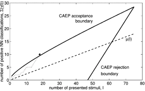
se-quential test is shown in Fig. 4. There, the abscissa represents the number of single sweep measurements, , the ordinate the sum of binary NN classifications. The upper limit in this
example is 75. If after sweeps exceeds the upper
Fig. 4. Sequential test plan with acceptance and rejection boundaries for assessment of NN classification (L =75 and p = 0.24); dashed line: mean value for the sum of positive NN classification for random sweeps; dotted line: example of sweep with CAEP detected afterl = 18 NN classifications.
stopped. If the lower boundary is reached after sweep record-ings, it becomes impossible that the upper boundary is met in the remaining sweeps, a CAEP is rejected and the mea-surement can be stopped. The dashed line in Fig. 4 shows the
mean value for positive NN-classifications in the
absence of a CAEP (type-I-error). An example for is given with the dotted line which, here, passes the acceptance boundary
( 10) after 18 sweep classifications, and a CAEP
is detected. It can be easily calculated that a minimum number of 3 sweep classifications is required before a CAEP can be detected under the conditions of this example.
The above sequential test procedure can be regarded as a semi-adaptive decision algorithm [29]. If the SNR of the CAEP inside the ongoing EEG is high enough, the algorithm will con-siderably shorten the time which is necessary to reach a deci-sion. However, if the SNR is extremely low, a larger number of measurements will be required. In case of the example given above, the test will need an average number of 62 sweeps until a measurement will be rejected as non-CAEP, as indicated by the intersection of the mean sum with the rejection boundary in Fig. 4.
III. ADJUSTMENT OFDETECTORUSINGREALDATA
Now, step by step, the general automatic detector outlined in Section II will be adjusted with respect to our data acquisition equipment and procedure, which is discussed in Section III-A. This has consequences for the tailoring of the DWT and the se-lection of transform coefficients parameterizing CAEPs in Sec-tion III-B. The subsequent dimensioning and training of the NN classifier is described in Section III-C. The false positive clas-sification rate of the NN together with a selected significance finally sets the parameters for tuning the sequential test in Sec-tion III-D.
A. Equipment and CAEP Data
All EEG measurements employed in this work were obtained under clinically proven conditions in an electrically insulated and acoustically anechoic chamber [31], where patients and ex-perimentees are seated in a comfortable armchair in order to
Fig. 5. Examples from the ensemble of synthetic CAEPs for additional NN training.
minimize motoric artifacts inside the EEG. The vigilance of per-sons under test is ensured by monitoring with a video system. The stimulation system (ASTI20, ZLE Corp., Munich) used here produces predefined signals, which are presented via a headphone (Beyerdynamics DT48) to the test persons and pa-tients. The EEG is measured as a voltage from the ipsilateral mastoid (M1, M2) and a contralateral forehead position (FP1, FP2) of the stimulated ear against a ground electrode positioned on the center of the forehead (FZ). After differential EEG ampli-fication by approx. 80 dB, the analog EEG signal is prefiltered by Bessel filters of 4th order with a passband region between 1.6 Hz and 20 Hz. Finally, the stimulation system triggers a 12-bit analog-to-digital converter sampling at 640 Hz for synchronous digital recording, yielding 2 samples for 800 ms seg-ments of EEG represented within each sweep.
Sine-bursts of 300–ms duration at frequencies of 500 Hz, 1 kHz, 2 kHz, and 4 kHz were used as stimuli, with intensities set to 20-, 40-, 60-, and 80-dB sensation level (SL) for individual experimentees. For measurements without CAEP, the stimulus could also be set to zero. The stimuli were separated by ran-domized inter-stimulus intervals of about 1–2 s to avoid artifacts through periodic repetition. For each stimulus situation a set of at least 75–100 sweeps was recorded. Hence, a complete mea-surement for one stimulus situation—defined by the stimulus frequency, stimulus level and the side of the stimulated ear—ex-tends over a duration of 2–3 min.
A set of 600 real CAEP measurements recorded with the above equipment was available for the adjustment of the de-tector. These measurements had been performed in the clinical routine on adult patients with a known psychoacoustic hearing threshold. The presence of CAEPs had been clearly identified by a human expert. The selection of the 600 measurements was done such that stimulation levels between 20- and 80-dB SL were uniformly represented.
Besides the real measurements, 100 synthetic CAEP time se-ries were additionally produced for the later training of the NN. These simulated CAEPs consisted of a combination of subse-quent sine and cosine half-waves with different positions of the maxima and different time scales [32], with examples given in Fig. 5.
B. Feature Vector
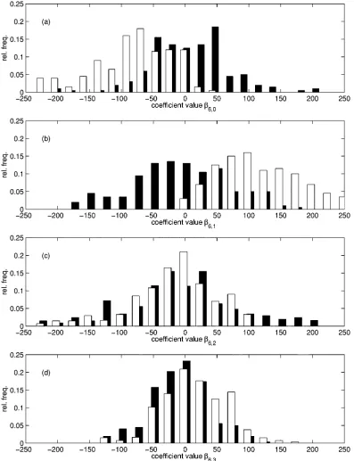
[image:5.612.298.554.62.152.2]Fig. 6. (a)–(d) Frequency distributions of coefficients , , , and , respectively, averaged over eight successive sweeps; white histograms refer to stimulus-synchronized sweeps (1 kHz, 80-dB SL), while black bars belong to coefficient values of data without given stimulus.
compared to the distribution of an EEG measurement with no CAEP. The comparison was realized by taking normally aver-aged and averaged sweeps, whereby the average was taken over a small sample size of eight successive sweeps. A wavelet with good parameterizing properties would then have at least one coefficient, for which a clear difference in the distributions for averaged sweeps could be measured [19].
From standard Daubechies wavelets, near-symmetric wave-lets [21], and Mallat’s wavelet [22], such testing gave best results for the Mallat wavelet with odd periodic extension of the data. This preference for odd extension is likely to be due to the
important components of a CAEP being close to the beginning of the sweep interval and, therefore, sensitive to discontinuities and wrap-around experienced with even periodic extensions [33]. Testing for other symmetric wavelets apart from Daubechies-2 (Haar) and Mallat wavelets was extended to a class of symmetric biorthogonal wavelets [24] which, however, did not produced better results than Mallat [34], [19].
Example: An example of the distributions measured for four
different Mallat-DWT coefficients ( , , , and )
in their distributions depending on the presence of a stimulus
(here, and ) while for others (here, and ) no
difference can be established. In this case, the first two coeffi-cients would be marked as “significant” for a CAEP.
With a measure how well the two distributions separate [19], not only was the Mallat wavelet determined amongst the library of wavelets tested over the data set, but the marking of “sig-nificant” coefficients would be mainly restricted to a subset of seven coefficients
(5)
This FV was optimized over all sweeps in the data set, and represents approximately the first 400 ms and the frequency
in-terval of a sweep. As this covers both
the latencies and the frequency range of 3–6 Hz generally asso-ciated with CAEPs [15], [35], the selection in (5) can be con-sidered robust in capturing the required information. However, not all coefficients in (5) have to be indicative for a CAEP in an individual measurement, as the above example demonstrated.
An initial detector [34] was based on measuring the separa-bility of distributions of averages over six to ten sweeps. This “separability” was based on the overlap and relative dis-tance of mean values of the distributions. If the separability for any coefficient of the set was above a predetermine threshold, a CAEP would be assumed. Over the data set, this gives a false positive error rate of approx. 9.8%. This method, however, re-quires an optimum a priori threshold selection, has no known confidence, and needs a fixed set of measurements [19]. Here, we use this experience as a motivation for the wavelet and coef-ficient selection for the FV, but want to use the systematic NN classification and sequential testing, which will be adjusted next based on the properties of the FV derived over the data set in Section III-A.
C. Dimension and Training of the NN
The FV of seven DWT-coefficients isolated in Section III-B encompasses the time-frequency range important for CAEPs and, therefore, can form the basis for further classification. Since the amplitude of the bioelectric brain signals largely depends on uncontrollable individual parameters of the test person’s vigilance and electrode impedances, no reliable infor-mation regarding CAEPs can be derived from the modulus of specific coefficients. Therefore, each FV was modified as de-scribed in Section II-B. The training of the NN was performed with FVs calculated from the 600 CAEP measurements and from 100 simulated CAEP time series, as outlined in Sec-tion III-A. Besides these FVs containing a CAEP, the learning group included 700 random FVs representing measurements without CAEP.
Different numbers of hidden neurons were used for the training in order to separate the CAEP from the non-CAEP in order to achieve best performance in the sense outline in Section II-B. With hidden neurons the classification for the training data was poorer in the sense that not all of the
FVs containing a CAEP were correctly classified. With 8 hidden neurons 100% of the CAEP and about 76% of the FV from the non-CAEP set were correctly classified. A further increase in the number of hidden neurons, , gave better results for the part of the learning set not containing a CAEP, but would decrease generalization due to the limited amount of sample FVs. The excitation of the NN with a restricted set of training data leads to adaptation of the NN parameters to this special data and is, therefore, only optimal for the training case. Hence, a number of 8 hidden neurons was selected as optimal choice for our classification problem.
In order to evaluate the precise false positive rate of the NN, Monte-Carlo simulations were performed using 10 random input vectors. The positive classification rate for these FV was determined to be 0.24, and proved to be very stable over repeated trials of this experiment.
D. Sequential Test Setup
Once the NN is trained, the false positive rate, 0.24, is fixed, as determined in Section III-C. The sequential test has to check whether the actual positive rate of the NN, , is sig-nificantly higher than the rate . Two parameters of the se-quential test proposed in Section II-C have to be preset. As max-imum number of NN-classification, 75 appears a reason-able number in the light of the usual 30–80 sweeps required for averaging CAEP measurements. The false positive rate (signifi-cance ) of the complete sequential test was selected to be 0.05.
With 0.05 and the known false positive rate 0.24 of NN classifications, can be adjusted. A rough and very conservative estimate for can be derived using the Bonfer-roni-correction [36], resulting in a approximation 3.02. A tighter approximation for can be found by Monte Carlo simulation.
For the Monte Carlo simulation, successive NN-classifica-tions of an EEG measurement with no stimulation and 0.24 were simulated by drawing from a random variable
uni-formly distributed on the interval and applying
the Heavyside function. A resulting value of “0” represents “no CAEP detected,” while “1” represent “CAEP detected.” With a total number of 500 000 random series, each containing 75 dichotome classification results , sequential tests were simulated with an a priori probability for positive
classifica-tions of 0.24. By running the factor from zero to
five in steps of 0.001, was determined such that the sum of NN classifications exceeds the limit at least at one time
in 5% of all series
(6)
where and are defined as in (3) with substituted for . In order to satisfy a 5% type-I-error probability, the numerical simulation resulted in the choice 2.83. Repeated Monte Carlo trials resulted in variations of of less than 0.01. Hence, in the proposed CAEP detector, the parameter
IV. CLINICALEVALUATION ANDDISCUSSION
The proposed sequential detector adjusted in Section III was evaluated in a clinical study, which is discussed in the following. Section IV-A introduces the study group and the measurements taken. The automatic detector is compared to a human expert in CAEP classification in an experiment, for which the conditions are set out in Section IV-B. Section IV-C presents and discusses the results.
A. Subjects
Eleven normal hearing volunteers (five male, six female) took part in the study. The experimentees were students at the Uni-versity of Erlangen-Nürnberg with an average age of
years. The subjects had no indication of hearing deficiencies or neurological diseases and did not take any drugs the day prior to investigation. Their normal hearing status was established by pure tone audiometry, where the hearing loss at all frequencies between 125 Hz and 10 kHz was less than 10 dB. Addition-ally, psycho-acoustical thresholds for the stimulus levels used to evoke CAEPs were determined with the same apparatus. The stimulus levels mentioned in the following represent the levels with respect to the individual hearing thresholds, indicated by decibel sensation level (dB SL).
A total of 32 EEG measurements were obtained form each experimentee, to account for all combinations of four different stimulus level (20-, 40-, 60-, and 80-dB SL), four different fre-quencies (0.5, 1, 2, and 4 kHz), and the testing of both ears. Each measurement consisted of 75 EEG sweeps. In addition to these regular CAEP measurements, for each subject a number of 32 sets of EEG recordings were taken without any auditory stim-ulation but under otherwise identical conditions. For this case, again a minimum number of sweeps of 75 was recorded. Finally, all measurements were randomly ordered to exclude inference from previous decisions on the current measurement under test.
B. Test Setup and Comparison with a Human Operator
For the study, the available measurements from the subject group introduced in Section IV-A totaled 352 data sets from EEG measurements with CAEP (stimulation above hearing threshold) and further 352 data sets without CAEP due to no given stimulus. Since the complete sets of single sweep responses were stored during the EEG recordings, the whole evaluation procedure can be performed off line. Thus, the above measurements were inspected 1) with the automatic method described in this paper and 2) by an experienced human operator. From the automatic CAEP recognition both the number of necessary stimulations for sequential detection and the result of the procedure (CAEP/no CAEP) were stored.
The human operator to evaluate the data was a member of sci-entific staff at the University hospital in Erlangen with 15 years of experience to classify CAEPs for objective hearing assess-ment in the clinical routine. This human operator was placed in a fully realistic situation for EEG recordings: for each stim-ulus condition (stimulated ear, stimulation level and frequency) the averages of subsequent sweeps in a measurement were cal-culated and displayed on a PC monitor. The timing of the dis-play was chosen similar to the interstimulus intervals during real
(a)
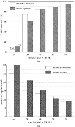
[image:8.612.300.555.60.494.2](b)
Fig. 7. (a) Decision rates for the automatic detector and those of an experi-enced human operator; (b) mean required number of sweeps in a measurement until a decision has been reached; a level of01–dB SL refers to no stimulus given.
measurements. However, the human operator was blind to the actual stimulus level of the presently displayed measurement and he had no information about the AEP at higher/lower level for the same subject. As soon as the operator was able to reach a decision, he could stop the measurement simulation, and both his decision and the required number of stimuli were recorded.
C. Results and Discussion
For the automatic detector, the type-I-error rate had been preset to 5% ( 0.05) as described in Section III-D. This closely agrees with the reached average false positive classi-fication (i.e., an CAEP is incorrectly assumed) of 5.9% for measurements with no given stimulus. It is clear from Fig. 7(a) that the human operator has a considerably higher type-I-error rate, even though he had been informed that half the measure-ments in the database contained no CAEP. This difference was evaluated as significant with the one-sided McNemar-Test [37] on a significance of 5%.
Looking at different stimulus levels, Fig. 7(a) shows a clear increase in the detection rate of CAEPs with the stimulation intensity for both the automatic sequential detector and the human operator, while the corresponding required measure-ment times in Fig. 7(b) decrease. This is due to the fact that stronger stimuli yield clearer pronounced CAEPs with larger amplitude and, thus, higher SNR, as shown in Fig. 1. Hence, detection becomes easier and faster. Differences in the classi-fication results between the human operator and the automatic recognition were significant for the detection rate of CAEPs at a 20-dB SL stimulus level, based the one sided McNemar-Test. Therefore for EEG measurements with a stimulus level close to the hearing threshold, the automatic sequential detector achieves a much sharper discrimination between measurements with and without CAEP than the human operator. The latter yields a 6% higher false positive rate for measurements without CAEP and a performance 15% below the false negative rate of the automatic detector for stimuli 20 dB above the known threshold of hearing. Concerning the decision time shown in Fig. 7(b), longer measurements in case of the human operator are due to hesitation in cases where the decision is difficult. The automatic sequential detector outperforms the human operator for most stimulus levels. The longest measurement times are necessary for the case of no acoustical stimulation, i.e., the absence of a CAEP from the EEG.
The CAEP classification by the human expert was repeated six months after the first assessment with the same data and method. From the total of 704 measurements 570 (81%) were identically classified in both situations. In more clinically ori-ented studies on assessment of hearing via CAEP measure-ments by other human operators “CAEP detection thresholds” are reported to vary between 16 dB [38] and 27 dB [39] above subjective hearing thresholds. The repeated decisions of the human operator consulted in this study were well within these limits.
Although the results obtained by the human operator should be representative for the state of the art in CAEP classification for hearing assessment in clinical routine, differences between the procedure in our study and the standard in clinical routine must be noted. First, the human operator in our study was in-formed about the a priori probability of 50% for a CAEP. As this information is unknown in clinical routine, generally the clinical assessment might be worse compared to decision rate in the study. Secondly, the CAEP analysis in clinical routine is usually based upon a set of CAEP measurements at different stimulus levels. This permits to see the dependency of ampli-tudes and latencies on stimulus levels, which can enhance the correct classification rates in the routine compared to our study.
It should further be noted that the human operator uses the accumulated sweep information differently from the sequential detection. His decision is based on linearly averaged sweeps, while the proposed detection method is based on binary non-linear classifications of single sweeps. For the later, the SNR of the data has to permit retrieval of sufficient information from single sweep data, as otherwise such classification would not be optimal. In the application to CAEPs evidently enough informa-tion is contained in single sweeps for decision making even at low stimulus levels.
In summary, the performance of the sequential classification can be regarded at least as good as the human operator. The rate of correct decisions of the automatic detector is identical to or higher than those attained by the human expert. Therefore, the proposed automatic sequential detector appears to give a supe-rior performance over an experienced human operator, yielding a more accurate decision in shorter time. The better discrim-ination for stimulation levels close to the hearing threshold is particularly important, as it enables to determine the objective audiogram more accurately.
V. CONCLUSION
We have introduced an automatic detection method for CAEPs, based on a DWT for feature extraction, a feature classification using a NN, and a decision mechanism based on a sequential statistical assessment of the NN’s output. Although the presented feature extraction by a dyadic DWT may not optimally represent the CAEP, and despite the very high type-I-error inherent in the NN classification, the final detector stage with the sequential test is able to produce satisfying results. Applied to a study, the comparison of our method to results obtained by an experienced human operator was favorable in reducing both decision errors and measure-ment time, particularly when operating with stimulus levels in the proximity of the hearing threshold. This underlines the suitability of the proposed approach, and the prospect to make clinical audiometric investigations via CAEP more accurate and faster.
Although there exists a considerable quantity of contributions dealing with the signal processing aspect for auditory evoked potentials, only few of these methods have been established in clinical routine since they are not adjusted to the clinical require-ments such as robustness for noisy data, restrictions on mea-surement duration, and exactly known rates of false positives. Clinically, the detection of a CAEP when no CAEP is present (type-I-error) is the most problematic case since it will result in failure to give, for example, a child the help it needs by erro-neously judging hearing to be present, at least in CAEP terms. Therefore, the appeal of the proposed automatic detector lies in its known statistical confidence, together with its good discrim-ination and the reduction in measurement time.
ACKNOWLEDGMENT
und Pädaudiologie, Universität Erlangen-Nürnberg, Germany, for discussion and their kind technical assistance.
REFERENCES
[1] S. Hoth, “Computer-aided hearing threshold determination from cortical auditory evoked potentials,” Scand. Audiol., vol. 22, no. 3, pp. 165–177, March 1993.
[2] A. Parving, C. Elberling, and G. Salomon, “Slow cortical responses and the diagnosis of central hearing loss in infants and young children,”
Scand. Audiol., vol. 22, no. 3, pp. 165–177, 1981.
[3] J. D. Durrant and J. H. Lovrinic, Bases of hearing science, 3rd ed. Baltimore, MD: Williams & Wilkins, 1995.
[4] N. Kraus, T. NcGee, A. Sharma, T. Carell, and T. Nicol, “Mismatch-negativity event related potential elicited by speech stimuli,” Ear Hear., vol. 13, pp. 158–164, 1992.
[5] R. Näätänen and T. Picton, “The N1 Wave of the Human Electric and Magnetic Response to Sound: A Review and an analysis of the compo-nent structure,” Psychophysiology, vol. 24, pp. 375–425, 1987. [6] J. W. Hall III, Handbook of Auditory Evoked Responses. Boston, MA:
Allyn & Bacon, 1992.
[7] P. Finkenzeller, “Die Mittelung von Reaktionspotentialen,” Kybernetik, vol. 6, pp. 22–44, 1969.
[8] C. Elberling and O. Wahlreen, “Estimation of auditory brainstem re-sponse, ABR, by means of Bayesian detection theory,” Scand. Audiol., vol. 14, no. 2, pp. 89–96, 1985.
[9] B. Lütkenhöner, M. Hoke, and C. Pantev, “Possibilities and limitations of weighted averaging,” Biol. Cybern., vol. 52, no. 6, pp. 409–416, June 1985.
[10] M. Wernicke, “Rekonstruktion von Akustisch Evozierten Hirnstamm-Potentialen,” Ph.D. dissertation, Technische Universität, Berlin, Ger-many, 1993.
[11] R. Mühler, “Experimentelle Untersuchungen und Modellrechnungen zur Reduktion der Reststörung bei der Registrierung auditorisch evozierter Potentiale früher Latenz,” Ph.D. dissertation, Univ. Olden-burg, OldenOlden-burg, Germany, 1997.
[12] G. H. Steeger, O. Herrmann, and M. Spreng, “Some improvements in the measurement of variable latency acoustically evoked potentials in human EEG,” IEEE Trans Biomed. Eng., vol. BME-30, pp. 295–303, May 1983.
[13] X. H. Yu, Y. Zhang, and Z. He, “Time-varying adaptive filters for evoked potential estimation,” IEEE Trans Biomed. Eng., vol. 41, pp. 1062–1071, Nov. 1994.
[14] , “Peak component latency-corrected average method for evoked potential waveform estimation,” IEEE Trans Biomed. Eng., vol. 41, pp. 1072–1082, Nov. 1994.
[15] S. Hoth and C. Weber, “Kritische Wertung der Hörschwellenbestim-mung Mittels der Hirnrindenpotentiale, Teil 1,” Audiol. Akustik, pp. 190–200, May 1990.
[16] H. Schimmel, “The+=0 reference: Accuracy of estimated mean com-ponents in average response studies,” Science, vol. 157, pp. 92–94, 1967. [17] M. J. Valdes-Sosa, M. A. Bobes, M. C. Prerez-Abalo, J. A. Carballo, and P. Valdes-Sosa, “Comparison of auditory-evoked potential detection methods using signal detection theory,” Audiology, vol. 26, pp. 166–178, 1987.
[18] E. A. Bartnik, K. J. Blinowska, and P. J. Durka, “Single evoked potential reconstruction by means of wavelet transform,” Biol. Cybern., vol. 67, no. 2, pp. 175–181, Feb. 1992.
[19] S. Weiss and U. Hoppe, “Recognition and reconstruction of late audi-tory evoked potentials using wavelet analysis,” in Proc. IEEE Int. Symp.
Time-Frequency and Time-Scale Analysis, Paris, France, June 1996, pp.
473–476.
[20] H. Dickhaus and H. Heinrich, “Classifying biosignals with wavelet-net-works,” IEEE Eng Med. Biol. Mag., vol. 15, pp. 103–111, Jan. 1996. [21] I. Daubechies, Ten Lectures on Wavelets. Philadelphia, PA: SIAM,
1992.
[22] S. G. Mallat, “A theory for multiresolution signal decomposition: The wavelet representation,” IEEE Trans Pattern Anal. Machine Intell., vol. 11, pp. 674–692, July 1989.
[23] R. E. Crochiere and L. R. Rabiner, Multirate Digital Signal
Pro-cessing. Englewood Cliffs, NJ: Prentice-Hall, 1983.
[24] M. Vetterli and C. Herley, “Wavelets and filter banks: Theory and de-sign,” IEEE Trans Signal Processing, vol. 40, pp. 2207–2232, Sep. 1992.
[25] G. Strang and T. Nguyen, Wavelets and Filter Banks. Wellesley, MA: Wellesley—Cambridge, 1996.
[26] C. Herley, “Boundary filters for finite–length signals without border dis-tortions,” IEEE Trans Circuit Syst. II, vol. 42, pp. 102–114, Feb. 1995. [27] A. Cichocki and R. Unbehauen, Neural Networks for Optimization and
Signal Processing. Chichester, U.K.: Wiley, 1993.
[28] S. Haykin, Neural Networks: A Comprehensive Foundation, 2nd ed. Englewood Cliffs, NJ: Prentice-Hall, 1998.
[29] K. S. Fu, Sequential Methods in Pattern Recognition and Machine
Learning. New York: Academic, 1968.
[30] R. G. Miller, “Sequential signed-rank test,” J. Amer. Stat. Assoc., vol. 65, no. 332, pp. 1554–1561, Dec. 1970.
[31] U. Hoppe, “Beiträge zur Bestimmung des Hörvermögens Mittels Audi-torisch Evozierter Potentiale,” Ph.D. dissertation, Univ. Erlangen-Nürn-berg, Germany, 1997.
[32] E. Fischer, “Untersuchungen zur Anwendbarkeit Neuronaler Netze bei der Klassifikation Akustisch Evozierter Potentiale,” Diplom thesis, Uni-versität Erlangen-Nürnberg, Germany, June 1995.
[33] W. H. Press, S. A. Teukolsky, W. T. Vetterling, and B. P. Flannery,
Numerical Recipes in C, 2nd ed. Cambridge, U.K.: Cambridge Univ. Press, 1992.
[34] S. Weiss, “Rekonstruktion Akustisch Evozierter Potentiale,” Diplom thesis, Univ. Erlangen-Nürnberg, Germany, Dec. 1994.
[35] S. Hoth and C. Weber, “Kritische wertung der hörschwellenbestimmung mittels der hirnrindenpotentiale, teil 2,” Audiol. Akustik, pp. 244–256, June 1990.
[36] R. G. Miller, Simultaneous Statistical Inference. Berlin, Germany: Springer-Verlag, 1981.
[37] J. Hartung, Statistik, 3rd ed. Munich, Germany: Oldenbourg-Verlag, 1985.
[38] D. Stapells, “Studies in Evoked Potential Audiometry,” Ph.D. disserta-tion, Univ. Ottawa, Ottawa, ON, Canada, 1984.
[39] M. I. Mendel, E. C. Hosick, T. R. Widman, and H. Davis, “Audiometric comparison of the middle and late components of the adult auditory evoked potentials awake and asleep,” Electroenceph. Clin. Neurophys., vol. 38, pp. 27–33, 1975.
Ulrich Hoppe (M’98) received the degree of Diplom-Physiker (M.S.) degree in physics from the University of Göttingen, Göttingen, Germany, in 1993 and the Ph.D. degree in engineering from the University of Erlangen-Nürnberg, Erlangen, Germany, in 1997.
Until 2000, he held a Postdoctoral position at the Department of Otorhinolaryngology of the University of Saarland, Homburg, Germany. Since 2000, he has been a Senior Scientist and Lecturer at the Department of Phoniatrics and Pediatric Audiology of the University of Erlangen-Nürnberg. His main research interests include biomedical modeling and signal processing, audiology, and medical pattern recognition.
In 2000, Dr. Hoppe received the Anelie-Frohn-Award from the German So-ciety of Phoniatrics and Pedaudiology (DGPP). He is Member of IEEE and the German Society of Medical Physics (DGMP) and the German Society of Audi-ology (DGA).
Stephan Weiss (S’97–A’98–M’99) received the Diplom-Ingenieur degree from the University of Erlangen-Nürnberg, Erlangen, Germany, in 1995 and the Ph.D. degree from the University of Strathclyde, Glasgow, Scotland, in 1998, both in electronic and electrical engineering.
Since 1999, he has been Research Lecturer in the Communications Group at the University of Southampton, prior to which he held a Visiting Lectureship at the University of Strathclyde. In 1996/1997, he was a Visiting Scholar at the Uni-versity of Southern California, Los Angeles. His research interests are mainly adaptive filtering, multirate systems, and signal expansions, with applications in audio, communications, and biomedical signal processing.
Robert W. Stewart (S’87–M’89) received the B.Sc. and Ph.D. degrees from the Department of EEE, Uni-versity of Strathclyde, Glasgow, Scotland, in 1985 and 1989, respectively.
He is a Senior Lecturer in the Department of EEE, University of Strathclyde. He was a Visiting Faculty at the University of Minnesota, Minneapolis, in 1990, a Research Assistant at the University of Strathclyde in 1987–1989, a Research Assistant at the University of Southern California, Los Angeles, in 1986–1987, and a Design Engineer with Wolfson Microelectronics Ltd. Since 1997, he has also been a part-time Visiting Professor at the University of California Los Angeles Extension School where he presents a course on Digital Signal Processing. He manages a research group in the general area of adaptive digital signal processing algorithms, DSP communication strategies, and real time implementations.
Dr. Stewart is a Member of the IEE. He is the webmaster for EURASIP.
Ulrich Eysholdt was born in Göttingen, Germany, in 1949, where he read Applied Physics and Medicine, and was a Ph.D. Student with M. R. Schroeder. He received both M.D. and Ph.D. degrees from the Uni-versity of Göttingen and specialized in the fields of ENT, phoniatrics and medical physics.
Since 1990, he is the head of the Department of Phoniatrics and Pedaudiology in the Faculty of Medicine at the University Erlangen-Nürnberg, Erlangen, Germany. At the same university, he holds a joint appointment with the faculty of Engineering Sciences since 1998. His research focuses on quantitative voice analysis and acoustical communication.