On an application of extended kalman filtering to activated sludge processes: a benchmark study

10th International Conference on Urban Drainage, Copenhagen/Denmark, 21-26 August 2005

On an application of extended Kalman Filtering to activated

sludge processes: A benchmark study

F. Benazzi1*, U. Jeppsson2 and R. Katebi1

1

Industrial Control Center, Department of Electronic and Electrical Engineering, University of Strathclyde, 50 George Street, Glasgow G1 1QE, UK

2 _{Industrial Electrical Engineering and Automation, Lund University, Box 118, SE-221 00}

Lund, Sweden

*Corresponding author, e-mail [email protected]

ABSTRACT

The growing demand for performance improvements of urban wastewater system operation coupled with the lack of instrumentation in most wastewater treatment plants motivates the need for non-linear observers to be used as virtual sensors for estimation and control of effluent quality. This paper is focused on the development of a general procedure for on-line monitoring of activated sludge processes, using an extended Kalman filter (EKF) approach. The Activated Sludge Model no.1 (ASM1) is selected to describe the biological processes in the reactor. On-line measurements are corrupted by additive white noise and unknown inputs are modelled using fast Fourier transform (FFT) and spectrum analyses. The given procedure aims at reducing the original ASM1 model to an observable and identifiable model, which can be used for joint non-linear state and parameter estimations. Simulation results are presented to demonstrate the effectiveness of the proposed methods and show that on-line monitoring of SND and XND concentrations is achieved when dynamic input data are used to characterize the influent wastewater for the model.

KEYWORDS

Activated sludge; extended Kalman filter; observability; software sensor; wastewater treatment

INTRODUCTION

Wastewater treatment plant (WWTP) control is an active area of research since two decades ago where mathematical models play an important role in understanding the control and operation of the systems. Wastewater treatment processes are generally described by complex non-linear systems that represent biological, physicochemical and biochemical processes. A model which is commonly used and considered state of the art for modeling biological nitrogen removal processes is the Activated Sludge Model No. 1 (ASM1) of the International Water Association (IWA) (Henze et al., 2000).

expensive. Therefore, the use of mathematical models is essential to develop “software sensors” and to enhance on-line performance monitoring and/or automatic control strategies. A “software sensor” (also called state and/or parameter estimator) can be described as a combination of a sensor (hardware) and an estimation algorithm (software), which is used to provide on-line estimations of specific states and/or kinetic parameters. Exploiting all information contained in the measurements supplied by on-line sensors, the “software sensor” performance is related to the process knowledge described by mathematical models. These types of sensors are often based on non-linear observer theory and have been successfully implemented in several cases (e.g. Benazzi et al., 2005; Bernard et al., 2000; Chéruy, 1996). However, it is extremely difficult to discern correct performance evaluation due to the non-uniformity of the simulated plant. Different models are used, combined with different parameter configurations, and most applications do not specify the kind of data used as influent to the WWTP. Therefore, this paper proposes a general procedure for on-line monitoring of activated sludge processes during wet-weather conditions (rain or storm events), using a “software sensor” based on an extended Kalman filter (EKF). The ASM1, where storm events are considered as influent, is selected to describe the biological processes in the activated sludge reactor.

The outline of the paper is as follows: A short introduction to the benchmark plant is provided, since this plant was selected as a suitable case study for this paper. A design procedure, as well as assumptions made, to obtain the reduced-order observable model is proposed. In the result section, joint state and parameter estimations are presented. Finally, some general conclusions are given.

IWA/COST SIMULATION BENCHMARK

Plant layout and process models

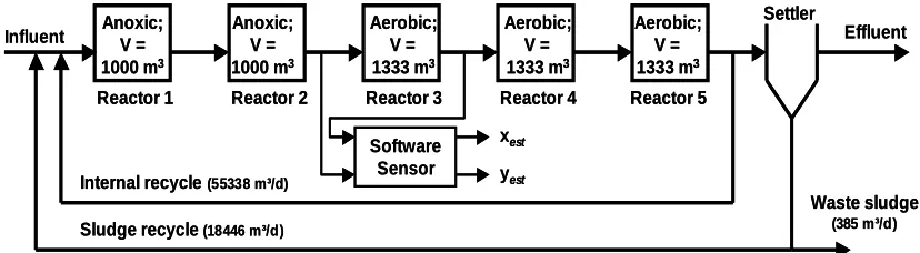
Only a short description of the benchmark plant and its process models is provided. For further information the reader should refer to Copp (2002). As seen in Figure 1, the original benchmark plant is considered to be the real plant and the “software sensor” is implemented on the first aerated reactor. The locations of the on-line sensors are not described and are beyond the scope of this paper. The ASM1 is selected to describe the biological processes in the activated sludge reactors. A ten-layer one-dimensional settler model applying the double-exponential settling velocity function proposed by Takács et al. (1991) is chosen to describe the settling process.

Influent

Reactor 1 Reactor 2 Reactor 3 Reactor 4 Reactor 5

Settler

Effluent

Internal recycle (55338 m³/d)

Sludge recycle (18446 m³/d)

Anoxic; V = 1000 m3

Waste sludge

(385 m³/d)

Anoxic; V = 1000 m3

Aerobic; V = 1333 m3

Aerobic; V = 1333 m3 Aerobic;

V = 1333 m3

Software Sensor

xest

yest Influent

Reactor 1 Reactor 2 Reactor 3 Reactor 4 Reactor 5

Settler

Effluent

Internal recycle (55338 m³/d)

Sludge recycle (18446 m³/d)

Anoxic; V = 1000 m3

Waste sludge

(385 m³/d)

Anoxic; V = 1000 m3

Aerobic; V = 1333 m3

Aerobic; V = 1333 m3 Aerobic;

V = 1333 m3

Software Sensor

xest

yest

10th International Conference on Urban Drainage, Copenhagen/Denmark, 21-26 August 2005

The storm influent wastewater data, which is a variation of the dry-weather data (normal diurnal variations) with two different storm events added, are used to characterize the influent wastewater for the model. In this work, it is assumed that the ASM1 is valid for moderate storm-weather conditions. The first event is of high intensity and short duration and is expected to flush the sewer of particulate material, and the second assumes that the sewers were cleared of particulate matter during the first event. Therefore, only a modest increase in the COD load can be observed during the second storm (Copp, 2002). All simulations are performed using the Matlab/Simulink platform, based on the defined open-loop benchmark configuration.

Non-linear observability

Observability is an important structural property of dynamic systems defined as the probability to infer the state of the system from examining its input and output relationships (and possibly their derivatives). The conditions of observability can govern the subsistence of a full solution to the control system design problem. Therefore, if the system is not observable, solutions to solve the control system design may not exist. Consequently, it is important to investigate the global or local observability of the model under study prior to the observer design. For further details about non-linear observability, the reader is referred to Isidori (1985).

Design procedure

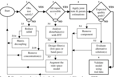
The flow chart diagram presented in Figure 2 illustrates the general procedure for on-line monitoring of activated sludge processes. With reference to the numbers given in Figure 2, the procedure is detailed as follows:

1. Select an appropriate ASM model (initialise and calibrate it) and evaluate the effluent quality goal.

2. Is the model globally observable (all initial condition must be determined uniquely from the output(s) and input(s) in the whole domain of definition)? Or

Is the model locally weakly observable (full rank in the whole domain of definition)? If not, then:

2.1 Reduce the ASM following one of the two different techniques:

2.1a Use a matrix decoupling technique, which allows the user to identify which component(s) is/are not affecting the model.

2.1.b Remove non-essential state variable(s) that is/are not relevant in the specific process (based on experience).

3. Are all plant inputs accessible? If not, model the unknown input(s) (also called disturbances in this paper) using the following technique:

3.1 Use FFT analysis on the disturbance(s) data to produce the disturbance spectrum.

3.2 Design/fit a/some filter(s) (low pass or band-pass), which approximates the frequency spectrum of the disturbance(s).

3.3 Augment the disturbance(s) state-space model to the main filter(s)/”software sensor(s)”.

4. Apply EKF to compute joint state and parameter estimations. 5. Expected quality goal achieved? If not, then:

5.1 Remove component(s) that are not relevant for the process.

5.2 Evaluate alternative solution(s) (e.g. is the augmented model observable? If not, go to Step 1).

Reduce ASM

Matrix decoupling

Analyse disturbance(s)

with FFT

Design filter(s) (low-pass or

band-pass)

Augment the state space

model

Remove component

Validate model

using real data

6 2.1

2.1.b

3.1

3.2

3.3

5.1

Evaluate alternative solution(s)

5.2

Remove concentration(s)

2.1.a

Expected quality goals? Obs.

test satisfy?

All inputs accessible

?

Apply joint state & param.

estimations Start

NO NO NO

Figure 2. General procedure to design “software sensor(s)” based on an EKF.

Reduced-order model used by the software sensor (EKF)

Following the procedure step 2.1b (see Figure 2), the following considerations were made to produce a reduced-order model, using the ASM1 as a starting point. Soluble inert organic matter (SI) contributes to the effluent chemical oxygen demand (COD), and particulate inert organic matter (XI) becomes a part of the total suspended solids in the activated sludge system. However, both SI and XI are excluded from the reduced model because they do not contribute to any other reactions and are not actively involved in any conversion processes. Inclusion of the particulate products arising from biomass decay (XP) in the ASM1 is an approach to account for the fact that not all biomass in the activated sludge system is active (Henze et al., 2000). Description of alkalinity (SALK) in the ASM1 is not essential (no impact on biological transformations) but its incorporation is sometimes advantageous because it provides information by which excessive change in pH can be predicted (Henze et al., 2000). Therefore, these two components are also excluded from the reduced model. Slowly changing variables are assumed constant, which means that the active heterotrophic (XBH) and autotrophic biomass (XBA) are kept constant in the reduced model, similarly to the model described by Ingildsen (2002). Consequently, the extended Kalman filter (EKF)-based observer (or “software sensor”) includes seven state variables, which are: readily and slowly biodegradable substrate (SS and XS), dissolved oxygen (SO), nitrate and nitrite nitrogen (SNO), NH4+ + NH3 nitrogen (SNH), soluble biodegradable organic nitrogen (SND) and particulate biodegradable organic nitrogen (XND) concentrations.

Software sensor implementation

10th International Conference on Urban Drainage, Copenhagen/Denmark, 21-26 August 2005

“WWT plant” Benchmark plant (13 state

variables)

(noise added)

Influent

SOFTWARE SENSOR

REDUCED-ORDER MODEL composed of 5 state variables:

XS, SO, SNO, SNH, XND +

TWO AUGMENTED STATE VARIABLES:

SS, SND

Disturbances filters design noise ˆ ND(t) S ˆ ND(t) X Selected inputs

to reactor 3 SO,in

SNO,in SNH,in Qin KLain

SO,in SNO,in SNH,in

On-line measurements from reactor 3

XS From respirometer Estimated concentrations ˆ S(t) S ˆ S(t) X ˆ O(t) S ˆ NO(t) S ˆ NH(t) S

Figure 3. Software sensor design: The dotted box represents the procedure that must be performed prior to the “software sensor” implementation.

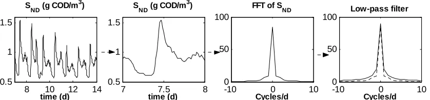
All concentrations estimated by the “software sensor” and its implementation, including state variables that are measured on-line as well as state variables that are not available (e.g. SS, SND), are presented in Figure 3. The unavailable states, referred to as disturbances in this paper, are analysed using fast Fourier transform (FFT) and spectrum analysis techniques prior to the “software sensor” implementation. This method is based on designing filter(s), which cover the frequency spectrum of the disturbances as represented in Figure 4. Firstly, dynamic SND concentration profiles were obtained in the time domain by simulating the benchmark plant for a period of seven days. On the resulting influent data (into the first aerobic reactor), a FFT was applied to convert the set of uniform space points from the time domain to the frequency domain in order to obtain the spectral content of the signal, and to design the appropriate filter. Secondly, a first-order low-pass filter was designed and properly tuned, where its output was used as an augmented state. Finally, the “software sensor” was implemented in parallel with the benchmark plant. It can be observed that this technique was applied over a period of one day (for simplification reasons), to capture the diurnal influent wastewater data dynamics. This FFT technique is applied in the first place theoretically (using the benchmark plant) on the unavailable concentrations such as SS and SND because access to these historic data is impossible in practice. Then, once the outputs of the low-pass filter are obtained and tuned, the “software sensor” can be implemented in practice. This FFT approach is extensively used to estimate non-measurable concentrations using simulated data (from the benchmark plant in this case). For further details about the observer algorithm (joint state and parameter estimation), the reader is referred to Dochain (2001; 2003).

8 10 12 14

0.5 1 1.5

S

ND (g COD/m 3

)

time (d) 7 7.5 8

0.5 1 1.5

S

ND (g COD/m 3

)

time (d) -10 0 10

0 50 100

FFT of S ND

Cycles/d -10 0 10

0 50

100 Low-pass filter

Cycles/d

Variance (σ)

Delay (min.)

Low-level detection limit

Sampling time (min.)

Oxygen (SO,ef) 0.172 - 0.1 continuous

Nitrate and nitrite nitrogen (SNO,ef) 0.654 10 0.1 10

NH4+ +NH3 nitrogen (SNH,ef) 0.5548 10 0.2 10

Influent (= effluent) flow rate(Q3,in) - - - continuous

Slowly bio. substrate (XS) 6.4855 30 0.1 30

RESULTS AND DISCUSSION

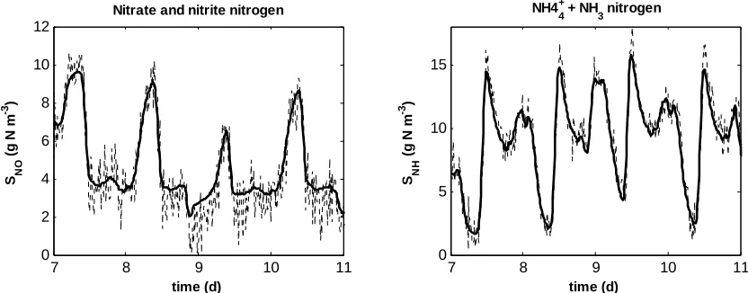
The “software sensor” was implemented following the design procedure described above. Initially, the non-linear observability of the reduced-order model was tested by computing the Lie-derivatives (computation of the outputs derivatives along the trajectories of the non-linear reduced-order model). Subsequently, two low-pass filters where designed to cover the energy of the unknown inputs (SS and SND). Finally, the “software sensor” was designed in order to provide on-line estimation of joint states and parameters. The XS concentration was assumed available from a respirometer with a delay of 30 minutes between each analysis, supposing that the concentration remain constant between two measurements. The “software sensor” estimated SS and XS and their respective concentrations were used on-line in the reduced-order model. Nitrogen (SNO) and ammonia (SNH) concentrations estimated by the “software sensor” are presented in Figure 5, with a standard deviation of 2.2 and 3.56 g N/m3, and a maximum bias of 2.78 and 0.01% occurring during the high intensity event, respectively. It can also be seen (from Figure 5) that the measurement noise is almost entirely filtered by the “software sensor”. Therefore, results show that realistic control strategies, where nitrogen and/or ammonia concentrations are corrupted by white noise, can be implemented using the estimation from the “software sensor” as feedback for PID and/or predictive control. Particulate nitrogen estimation was obtained assuming a ratio of XND to XS of 6.2%. Results displayed in Figure 6 show that SND and XND are estimated on-line by the “software sensor” with a standard deviation of 0.21 and 1.96 g N/m3, and a maximum bias of 0.007 and 0.002% occurring during the high intensity event, respectively.

7 8 9 10 11

0 2 4 6 8 10 12

Nitrate and nitrite nitrogen

S NO

(g

N

m

-3 )

time (d)

7 8 9 10 11

0 5 10 15

NH4

4 +

+ NH

3 nitrogen

S NH

(g

N

m

-3)

time (d)

10th International Conference on Urban Drainage, Copenhagen/Denmark, 21-26 August 2005

7 8 9 10

0.6 0.8 1 1.2 1.4 1.6 1.8

Soluble organic nitrogen

S ND

(g

N

m

-3 )

time (d)

7 8 9 10

2 4 6 8 10 12 14 16

Particulate organic nitrogen

X ND

(g

N

m

-3)

time (d)

Figure 6. Comparison between SND and XND concentrations resulting from simulations with the ASM1 model (dashed line) and estimated SND and XND concentrations by the “software sensor” implemented on the benchmark plant (solid line).

The lag time between the true state values and the “software sensor” estimates are attributed to off-line analysis and on-line measurements delay coefficients introduced in the simulation parameters (see Table 1).

The initial benchmark plant has been designed assuming that all kinetic and stoichiometric coefficients are constants, which is not obvious in a real wastewater treatment plant. Therefore, parameter estimations aim to provide values for the parameters in the model, depending on the quality of the experimental data set available. Coefficient (or parameter) estimation results are presented in Figure 7 for a11 and a22 parameters. These results present non-linear combinations of some traditional model parameters and give an idea of how some amalgamated model parameters act. The remaining coefficients of the system matrix (A matrix) contained in the state-space representation of the reduced-order model behave in a similar manner. A parameter estimation algorithm could probably be implemented in the “software sensor” for kinetic parameter identification (e.g. the heterotrophic growth rate) although this has not been tested yet and is beyond the scope of this paper.

8 8.5 9 9.5 10

4 6 8 10 12

a11

time (d)

8 8.5 9 9.5 10

-0.02 0 0.02 0.04 0.06 0.08

a22

time (d)

wastewater treatment plant rather than on the influent of the third reactor. The “software sensor” can also be used in the anoxic reactor (or on different aerobic tanks) by modifying the reduced-order model mass balance equations. It is important to estimate SND and XND on-line in order to: (1) include these concentrations in the process and obtain accurate information (e.g. of ammonia) and (2) develop robust control strategies in order to achieve efficient plant operation.

CONCLUSIONS

A general procedure for on-line monitoring of an activated sludge processes, using a “software sensor” based on an extended Kalman filter (EKF) has been proposed. On-line estimation of joint states and parameters demonstrates the effectiveness of the proposed method, based on a widely accepted process model, namely the ASM1. Results show that on-line monitoring of SND and XND concentrations is achieved when dynamic input data are used to characterize the influent wastewater for the model.

ACKNOWLEDGEMENTS

The authors wish to thank Dr. Darko Vrecko for insightful comments on the content of the paper. The financial support provided through the European Community’s Human Potential Programme under contract HPRN-CT-2001-00200 (WWT&SYSENG) is gratefully acknowledged.

REFERENCES

Alex J., Beteau J.F., Copp J.B., Hellinga C., Jeppsson U., Marsili-Libelli S., Pons M.N., Spanjers H. and Vanhooren H. (1999). Benchmark for evaluating control strategies in wastewater treatment plants. Proc. ECC’99 Conference, Karlsruhe, Germany, August 31-September 3, 1999.

Benazzi F., Katebi R. and Wilkie J. (2003). Application of Extended Kalman Filter to Activated Sludge Process. Internal publication, EU Research Training Network, HPRN-CT-2001-00200, Copenhagen Workshop (DTU, Denmark).

Benazzi F., Gernaey K.V., Jeppsson U. and Katebi R. (2005). On-line estimation and detection of abnormal substrate concentrations in WWTPs using a software sensor: A benchmark study. 2nd _{IWA conference on}

ICA, May 29-June 2, Busan, Korea (submitted).

Bernard O., Hadj-Sadok Z. and Dochain D. (2000). Software sensors to monitor the dynamics of microbial communities: application to anaerobic digestion. Acta Biotheoretica, 48, 197-205.

Chéruy A. (1996). Software sensors in bioprocess engineering. J. Biotechnol., 52, 193-199.

Copp J.B. (Ed.) (2002). The COST Simulation Benchmark. Description and Simulator Manual. ISBN 92-894-1658-0. Office for official publications of the European communities, Luxembourg.

Dochain D. (2001). State observation and adaptive linearizing control for distributed parameter (bio)chemical reactors. Int. J. Adapt. Control Signal Process., 15, 633-653.

Dochain D. (2003). State and parameter estimation in chemical and biochemical processes: a tutorial. J. Process Control, 13, 801-818.

Henze M., Gujer W., van Loosdrecht M. and Mino T. (2000). Activated Sludge Models ASM1, ASM2, ASM2d and ASM3. Scientific and technical report No 9, IWA Publishing, London, UK. ISBN-1 900222-24-8. Ingildsen P. (2002). Realising full-scale control in wastewater treatment systems using in situ nutrient sensors.

PhD thesis, Department of Industrial Electrical Engineering and Automation, Lund University, Lund, Sweden. ISBN 91-88934-00-4.

Isidori A. (1985). Nonlinear Control Systems. (Fettweis A., Massey J.L., Modestino J.W. and Thoma M. (2nd Edition)), pp 5-14, Springer-Verlag Edition, Germany.