An Adaptive Time Step Backward Differentiation Algorithm to Solve Stiff Ordinary Differential Equations: Application to Solve Activated Sludge Models

(1)

ISSN Online: 2161-1211 ISSN Print: 2161-1203

An Adaptive Time-Step Backward Differentiation

Algorithm to Solve Stiff Ordinary Differential

Equations: Application to Solve Activated

Sludge Models

Jamal Alikhani1,2_{, Bahareh Shoghli}3_{, Ujjal Kumar Bhowmik}1_{, Arash Massoudieh}2*

1_{Department of Electrical Engineering and Computer Science, The Catholic University of America, Washington DC, USA} 2_{Department of Civil Engineering, The Catholic University of America, Washington DC, USA}

3_{Department of Civil Engineering, University of North Dakota, Grand Forks, ND, USA}

Abstract

A backward differentiation formula (BDF) has been shown to be an effective way to solve a system of ordinary differential equations (ODEs) that have some degree of stiffness. However, sometimes, due to high-frequency variations in the external time series of boundary conditions, a small time-step is required to solve the ODE system throughout the entire simulation period, which can lead to a high computational cost, slower response, and need for more memory resources. One possible strategy to overcome this problem is to dynamically adjust the time-step with respect to the sys-tem’s stiffness. Therefore, small time-steps can be applied when needed, and larger time-steps can be used when allowable. This paper presents a new algorithm for ad-justing the dynamic time-step based on a BDF discretization method. The parame-ters used to dynamically adjust the size of the time-step can be optimally specified to result in a minimum computation time and reasonable accuracy for a particular case of ODEs. The proposed algorithm was applied to solve the system of ODEs obtained from an activated sludge model (ASM) for biological wastewater treatment processes. The algorithm was tested for various solver parameters, and the optimum set of three adjustable parameters that represented minimum computation time was identified. In addition, the accuracy of the algorithm was evaluated for various sets of solver parameters.

Keywords

Adaptive Time-Step, Backward Differentiation Formula, Activated Sludge Model, Ordinary Differential Equation, Stiffness, Computation Time

How to cite this paper: Alikhani, J., Shog-hli, B., Bhowmik, U.K. and Massoudieh, A. (2016) An Adaptive Time-Step Backward Differentiation Algorithm to Solve Stiff Ordinary Differential Equations: Applica-tion to Solve Activated Sludge Models. American Journal of Computational Ma-thematics, 6, 298-312.

http://dx.doi.org/10.4236/ajcm.2016.64031

Received: September 27, 2016 Accepted: November 8, 2016 Published: November 11, 2016

(2)

1. Introduction

The use of suspended microorganisms to remove undesired components, including or-ganic carbon, nitrogen, and phosphorus species, is referred to as activated sludge processes and is widely used around the world in municipal wastewater treatment

plants (WWTPs) [1] [2] [3]. Mathematical models of activated sludge processes,

re-ferred to as Activate Sludge Models (ASMs), provide a cost-effective way to evaluate design, control, and optimization of the processes and have been used extensively in practical applications and academic research [4] [5] [6] [7]. Henze et al. [8] proposed the first ASM (ASM1), and since then, several other versions of ASMs have been

pro-posed [9]. ASM1 represents wastewater composition using 13 constituents, where each

constituent may interact with each other through 8 reactions in which the general mass balance of each variable results in a system of ordinary differential equations (ODEs) describing the change in concentrations over time. Non-linear reaction rates based on Monod Kinetic cause a system of highly nonlinear ODEs. In some applications, the computation time of the ASM is critical due to a long simulation period, the need for

online simulation [10], and the use of parameter estimation algorithms that require

numerous simulations. For example, Alikhani et al. [11] modeled a large scale WWTP

with an ASM by using Markov-Chain Monte Carlo (MCMC) sampling and solved a large system of ODEs for 500,000 times to obtain the ASM’s parameter posterior prob-ability distribution. Therefore, applying a fast algorithm to solve ASMs that can signifi-cantly decrease the computation time of such applications would be highly desired. In addition to the non-linearity of the system of ODEs comprising ASMs, they typically cover a wide range of biochemical reaction rate scales, ranging from seconds (for ex-ample, oxygen transfer rate) to days (for exex-ample, microbial growth rates) and result in

a mixed (stiff/nonstiff) system of ODEs [12] that generally requires small time-steps

when conventional ODE solver algorithms are used. Furthermore, due to the inherent fluctuating behavior of the external forcing vectors, including variation in the time se-ries of the influent rate and the characteristics in wastewater treatment streams, the op-timal time-step size can vary greatly during the course of a simulation.

Explicit and semi-explicit ODE solvers have been shown not to perform well for sys-tems of ODEs with high degrees of stiffness, while backward differentiation formulas

(BDFs) have been shown to be much more suitable [13] [14] [15] [16]. In addition,

be-cause the degree of stiffness during the course of the simulation can vary, using a fixed but small time-step can translate to a heavy computational burden. A dynamically adaptive time-step algorithm can automatically adjust the time-step according to the degree of stiffness, resulting in a more optimal use of computational resources. For example, Celaya et al. [17] proposed a method to select or reject a proposed time-step in adaptive algorithms by evaluating the local truncation error at each time-step to maintain the error below a given threshold.

(3)

properly adjusting the solver parameters and can be used in other numerical method

applications such as advection-dispersion-diffusion equations solution [18], Bayesian

parameter estimation framework [19], and other application of numerical methods (e.g.

[20] [21] [22]). The proposed adaptive BDF algorithm in this study contains three ad-justable parameters that can be manipulated to achieve the minimum computation time for a given system of ODEs. In addition, a sensitivity analysis is conducted to identify the optimally adjustable parameters of the adaptive algorithm for a system of ODEs obtained for a sample ASM problem.

2. Methods

2.1. Adaptive Backward Differentiation Algorithm

The system of ODEs can be written in the following general form [23]:

( ) ( )

(

)

d

, ,

dt = t t t

C

f C U (1)

( )

t0 = 0,

( )

t is given

C C U

where, t is the time, C

( )

t is the state variables vector, and C0 is the initial condition.

( )

t

U is the boundary condition or the external forcing vector given for the entire

si-mulation period. The first and second order BDFs can be represented considering a va-riable time-step hi=ti+1−ti in a given time-step (i) as [17] [24]:

1

1 1 1 0

st

i+ = i+ − i−hi i+ =

F C C f (2)

2

1 1 1 1

1 1

1.5 1.5 0.5 0.5 0

nd i i

i i i i i i

i i h h h h h + + − + − −   = −_ + _ + − =  

F C C C f (3)

where i indicates the time-step with non-constant step size hi, fi = f

(

ti,C Ui, i

)

represents the discretized form of Equation (1) when Ci =C

( )

ti and Ui=U

( )

ti . In

Equations (2) and (3), 1

1 st i+

F and 2

1 nd i+

F are the first and second order BDFs

consider-ing non-constant step size at each time-step, respectively, which will be henceforth

de-noted as F for the sake of generality. The conventional Newton-Raphson (NR)

me-thod for solving the system of non-linear F to find C_i₊₁ can be formulated as:

( )1 ( ) ( )

1 1 1 1 k k l k

i i J i

− +

+ = + − × +

C C F (4)

where k is the iteration index beginning from 0, 1

l

J− is the inverse of Jacobian matrix (Equations (5) and (6)). Due to the fact that inverting the Jacobian matrix is computa-tionally intensive, especially as the size of the matrix grows, it is beneficial if the inverse of the Jacobian matrix can be reused and is recalculated only when necessary. Therefore, in the proposed method, Jl in Equation (4) is a recycled Jacobian matrix evaluated at some previous time tl.

(

)

1 , ,

I

l l l

st

l ij _{n n} l K

l _{n n}

(4)

(

)

2 , ,

1.5

I

l l l

nd

l ij n n l K

l _{n n}

f t

J h

c

δ _×

×

∂ 

 

= _{ } −  _∂ 

 

 

C U

(6)

where n is the size of the ODEs, δij is the Kronecker Delta, 1st l

J and J_l2nd denote

the Jacobian matrix for the first and second order F, respectively, where K

l

c is the Kth_{element of vector}

l

C , and similarly, I

f is the Ith element of vector f at tl. In addition, to further speed up the NR convergence, the following initial guess of the state variables is used at the first iteration (initial guess) of the NR [25]:

( )0 1

i+ = i+ ∆ i

C C C (7)

where ∆ =Ci Ci−Ci−1.

The adaptive time interval scheme adjusts the size of time-steps based on monitoring

the convergence of the NR method [25] [26]. The time-step size keeps growing by the

factor of 1 + ρ (ρ ≥ 0) until the NR’s iteration k in Equation (4) remains smaller than a

threshold kmax, and this inverse of Jacobian matrix ( 1

l

J− ) will be used in Equation (4). The iteration continues until the number of iterations to achieve convergence in the NR method exceeds kmax. At this time, a new Jacobian matrix will be computed and/or the

time-step size will be reduced by the factor of 1

1+γ (γ ≥0). Figure 1 depicts a de-

tailed flowchart of this algorithm, in which ρ, γ, and kmax are, respectively, the time-step inflation factor, the time-step depression factor, and the desired maximum iteration number of NR method that can be manipulated for each particular case of ODEs to achieve the minimum computation time.

2.2. Activated Sludge Model

(5)

[image:5.595.197.552.66.467.2]

Figure 1. Adaptive time-step BDF algorithm with adjustable parameters of ρ, γ, and kmax.

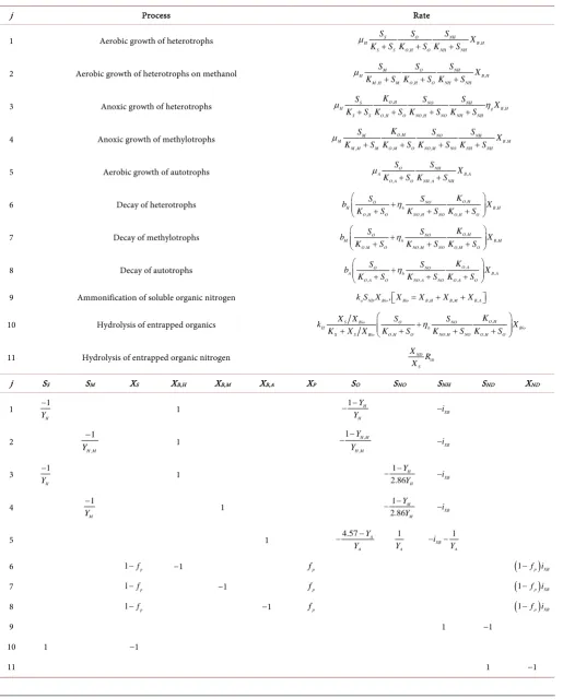
[image:5.595.199.550.505.662.2]

(6)

[image:6.595.44.560.84.725.2]

Table 1. Process reaction rates (R) and constituents stoichiometeries (∅).

j Process Rate

1 Aerobic growth of heterotrophs ,

,

S O NH

H B H

S S O H O NH NH

S S S

X

K S K S K S

µ

+ + +

2 Aerobic growth of heterotrophs on methanol ,

, ,

M O NH

H B H

M H M O H O NH NH

S S S

X

K S K S K S

µ

+ + +

3 Anoxic growth of heterotrophs ,

,

, ,

O H

S NO NH

H g B H

S S O H O NO H NO NH NH

K

S S S

X

K S K S K S K S

µ η

+ + + +

4 Anoxic growth of methylotrophs ,

,

, , ,

O M

M NO NH

M B M

M M M O M O NO M NO NH NH

K

S S S

X

K S K S K S K S

µ

+ + + +

5 Aerobic growth of autotrophs ,

, ,

O NH

A B A

O A O NH A NH

S S

X

K S K S

µ

+ +

6 Decay of heterotrophs ,

,

, , ,

O H

O NO

H h B H

O H O NO H NO O H O

K

S S

b X

K S η K S K S

 

+

 

 ₊ ₊ ₊ 

 

7 Decay of methylotrophs ,

,

, , ,

O M

O NO

M h B M

O M O NO M NO O M O

K

S S

b X

K S η K S K S

 

+

 

 ₊ ₊ ₊ 

 

8 Decay of autotrophs ,

,

, , ,

O A

O NO

A h B A

O A O NO A NO O A O

K

S S

b X

K S η K S K S

 

+

 

 ₊ ₊ ₊ 

 

9 Ammonification of soluble organic nitrogen k S Xa ND Bio,XBio=XB H, +XB M, +XB A, 

10 Hydrolysis of entrapped organics ,

, , ,

O H

S Bio O NO

H h Bio

X S Bio O H O NO H NO O H O

K

X X S S

k X

K X X K S η K S K S

 

+

 

+ _ + + + _

11 Hydrolysis of entrapped organic nitrogen 10

ND S

X R X

j SS SM XS XB,H XB,M XB,A XP SO SNO SNH SND XND

1 1

H

Y

−

1 1 H

H

Y Y

−

− −i_XB

2 , 1 H M Y −

1 ,

, 1 H M

H M Y Y − − XB i −

3 1

H

Y

−

1 1

2.86 H H Y Y −

− −i_XB

4 1

M

Y

−

1 1

2.86 M M Y Y −

− −i_XB

5 1 4.57 A

A Y Y − − 1 A Y 1 XB A i Y − −

6 1−fp −1 fp

(

1−fp

)

iXB

7 1−f_p −1 f_p

(

1−fp

)

iXB

8 1−fp −1 fp

(

1−fp

)

iXB

9 1 −1

10 1 −1

(7)

[image:7.595.47.553.63.355.2]

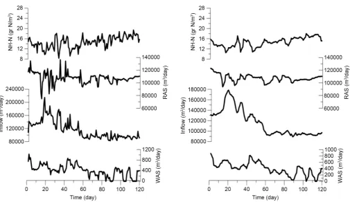
Figure 3. Influent flow and ammonia concentration, RAS and WAS over time: (Left) Unfiltered; (Right) Filtered using moving average technique over a 7-day span.

Governing ODEs

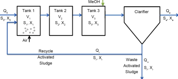
In ASMs, the activated sludge process is commonly represented as a series of attached, mixed reactors. These reactors hold a series of processes that can occur simultaneously, resulting in changes in the concentration of constituents. Figure 2 depicts a schematic of the activated sludge process of this study in the WWTP. A transient mass balance can be mathematically performed for each state’s variables, consisting of the concentra-tion of each model constituent, resulting in a system of ODEs, as expressed in Equaconcentra-tion (8). Therefore, Equation (8) expresses the changes in constituents’ concentrations over time as controlled by influents, effluents, reactions, and various mass-transfer processes

[9] [23]:

(

)

(

)

(

)

,

, , , , , ,

, , ,

*

, , , ,

1 d

d

m

r

N j m

m ret m ret j ret m in j in m m m m i m

m m N

m m m m j m

m m N

m r j r j m m m j m j m

r

C

V Q C Q C H Q Q C

t

H Q Q C

V R F V C C m

ω ω ′ ′ ′

′≠

′ ′

′≠

=

= + +

 

+_ − _

 

+ ∅ + − +

∑



(8)

(T−1_{) is the mass transfer rate,} *

C (M∙L−1) is the saturated concentration, and m (M∙L−1_{) is the external mass flow rate. And as for the indices, j indicates a constituent,} m represents a tank, “ret” indicates a return flow, “in” shows conditions in influent, and r indicates the reaction. In addition, Nm is the total number of tanks, and Nr is the total number of reactions. Qm m′, is the flow rate from tank m' to tank m, due either to

se-quential stages or through feedback or bypass (a positive Qm m′, value means to flow

into tank m). In Equation (8), the term on the left side is the rate of change in the total mass of the constituents j in tank m. The first term on the right side of Equation (8) is the mass inflow due to return flow; the second term is the mass inflow of the influent; the third term represents inflow from the preceding stage or feedback flow if it is present; the fourth term is the outflow of constituents; the fifth term is the production or disappearance of constituents due to reactions; the sixth term is the effect of rate-limited mass transfer (for example, aeration); and the last term is the direct addi-tion of the constituents (for example, the addiaddi-tion of a carbon source for denitrifica-tion). To obtain solid-particle concentrations in the return flow (Cj ret, ), a dynamic

cla-rifier model [27] or a quasi-steady-state approximation (that is, performing mass bal-ance while ignoring the solid storage changes in the clarifier) can be applied. The study described in this paper used the former approach.

3. Results and Discussion

The resulting system of ODEs, consisting of 15 state variables and 45 ODEs, was solved with a range of adjustable parameters for both unfiltered and filtered external vectors, and the running time for each set of solver’s parameters was recorded. The solver algo-rithm was implemented into the BioEst program, which was developed using the C++ language. The results presented in the next section were obtained by running the ex-ecutive version of the C++ code on a desktop computer with a quad-core Intel® 2.67 GHz Xenon® CPU and 8 Gb RAM.

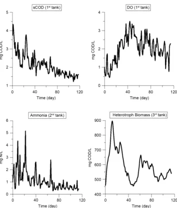
Figure 4 shows the results of the simulation for soluble chemical oxygen demand (sCOD), dissolved oxygen (DO), ammonia, and heterotroph biomass concentrations based on unfiltered influent obtained using the solver parameters ρ = 0.01, γ = 0.01, and kmax = 10.

3.1. Optimum Adjustable Parameters

To get the minimum computation time (running time) and acceptable accuracy, the user can assign the three adjustable parameters, including the inflation growth rate of the time-step (ρ), the depression rate of the time-step (γ), and the maximum NR’s ite-ration (kmax). A small initial time-step of h0 = 10−5_{day is chosen for all the cases. First,} the effect of changing ρ and γ is investigated by varying ρ between 0.0001 and 0.1 and γ between 0.0001 and 1 at the fixed kmax of 4. Figure 5 shows the results for effect of ρ and γ on running time. In both scenarios, filtered and unfiltered U

( )

t , the running time is

very sensitive to ρ, and the minimum running time occurs at ρ = 0.01. Figure 5 also

(9)

Figure 4. Results obtained for 120 days by using adaptive BDF method in a 3 tanks in series scheme with solver parameters of ρ = 0.01, γ = 0.01, and kmax = 10.

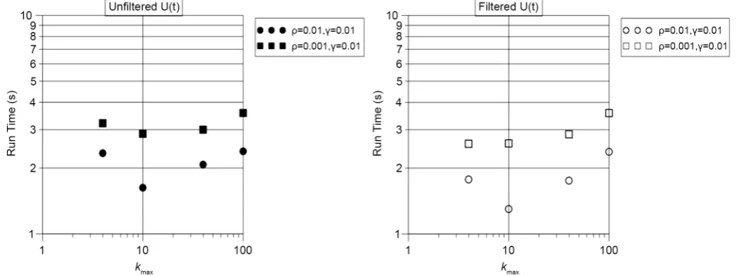
unfiltered scenarios. For example, at ρ = 0.01, in the case of unfiltered influent, γ = 0.01 gives a minimal running time and γ = 0.1 gives a similar running time, showing the low sensitivity of the algorithm to γ. The effect of the maximum number of iteration kmax is examined by assigning the values of 4, 10, 40, and 100. Figure 6 shows the effect of kmax on the running time for two sets of inflation-depression parameters. In both scenarios,

the algorithm shows a reasonably high sensitivity to kmax, and a minimum running time

occurs at kmax = 10. In conclusion, for the selected system of ODEs, the minimum

computation time is achieved at ρ = 0.01, γ = 0.01, and kmax = 10.

[image:9.595.196.551.63.479.2]

(10)

[image:10.595.46.554.68.266.2]

Figure 5. Effect of ρ and γ in a constant kmax = 4 in run-time for solving the system of 45 ODEs during 120 days. (Left) Unfiltered (t);

(Right) Filtered U(t).

Figure 6. Effect of kmax in run-time for solving the system of 45 ODEs during 120 days. (Left) Unfiltered (t); (Right) Filtered U(t).

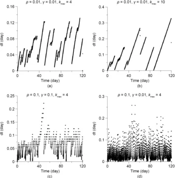
3.2. Variable Time-Step Pattern

The adaptive time-step algorithm increases the size of the time-step in the case when the NR algorithm continues converging and decreases the size of the time-step when the NR fails to converge. This pattern can be seen in Figure 7, which shows the varia-tion of the accepted time-steps during the course of the simulavaria-tion for four sets of ad-justable parameters. The results show that the pattern of variation in the time-step is substantially affected by different sets of adjustable parameters. For example, as Figure

7 shows, at kmax = 10, the time-step can reach a maximum value of 0.35 days, whereas,

[image:10.595.40.557.313.507.2]

(11)

Figure 7. Adaptive time-step (dt) variation for 120 days of applying adaptive BDF method on unfiltered U(t) for different adjustable parameters.

the effort needed in the Jacobian inverting process relative to the computational cost of NR iterations, which are mainly matrix-vector multiplications. Therefore, the optimal kmax can also depend on the size of the Jacobian matrix (that is, the number of state va-riables) and how well-posed the Jacobian matrix is.

As Figure 7 shows, at any given kmax, when γ is varied from 0.1 to 0.01, the pattern of

the time-step variation differs significantly and shows more fluctuation at a lower γ.

This indicates that the solver parameters ρ and γ essentially control how much the

time-step is increased or decreased. A smaller ρ and γ lead to more conservative

creases or decreases of the time-step and a larger ρ and γ lead to less conservative in-creases or dein-creases.

3.3. Error Assessment

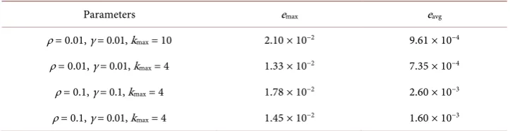
[image:11.595.195.552.72.435.2]

(12)

[image:12.595.193.555.101.194.2]

Table 2. Maximum and the average error of the ABDF algorithm using various parameter selec-tions as compared with RK4.

Parameters emax eavg

ρ = 0.01, γ = 0.01, kmax = 10 2.10 × 10−2 9.61 × 10−4

ρ = 0.01, γ = 0.01, kmax = 4 1.33 × 10−2 7.35 × 10−4

ρ = 0.1, γ = 0.1, kmax = 4 1.78 × 10−2 2.60 × 10−3

ρ = 0.1, γ = 0.01, kmax = 4 1.45 × 10−2 1.60 × 10−3

numerical error of the proposed adaptive BDF method can be evaluated. For this

rea-son, to evaluate the accuracy of the method, the well-known Runge-Kutta 4th_order

(RK4) method is used to solve the presented system of ODEs with a small constant time-step size. The selected time-step size is small enough that the truncation error

re-mains below 10−8_[26]_{. Then, the numerical results obtained from the RK4 method are}

used as a reference to assess the maximum and average error of the proposed adaptive BDF algorithm.

Since the oxygen mass transfer rate in Tank 1 is set at FO₂ = 190 day

−1_(Equation

(8)), resulting in the highest order of stiffness in the system of ODEs, the dissolved oxygen concentration in Tank 1 is susceptible to showing higher sensitivity to the ap-plied numerical method. Therefore, relative error is calculated based on the following equation:

( )

_{( )}

RK4

( )

RK4

So t So t

e t

So t

−

= ₍₉₎

where So t

( )

and So_RK4

( )

t show oxygen concentrations at Tank 1, obtained by the

proposed algorithm and RK4, respectively. Table 2 lists the relative maximum (emax)

and average (eavg) of e t

( )

for four sets of adjustable parameters. The accuracy assess-ment results show acceptable accuracy for the proposed algorithm. Specifically, for the four cases, the maximum and average errors contain less than 2 and 0.3 percent error, respectively.

4. Conclusion

(13)

model containing 15 constituents in each of 3 reactors. The sensitivity analysis is con-ducted, and the optimum adjustable parameters of the adaptive algorithm are identified. The accuracy analysis shows an acceptable level of accuracy for the proposed algorithm.

Acknowledgements

The authors would like to thank the Innovation section of the DC Water and Sewer Authority (DCWASA) for providing the data and financially support the research.

References

[1] Gernaey, K.V., van Loosdrecht, M.C.M., Henze, M., Lind, M. and Jørgensen, S.B. (2004)

Activated Sludge Wastewater Treatment Plant Modelling and Simulation: State of the Art.

Environmental Modelling & Software, 19, 763-783.

http://dx.doi.org/10.1016/j.envsoft.2003.03.005

[2] Hauduc, H., Rieger, L., Ohtsuki, T., Shaw, A., Takacs, I., Winkler, S., Heduit, A., Vanrol-leghem, P.A. and Gillot, S. (2011) Activated Sludge Modelling: Development and Potential Use of a Practical Applications Database. Water Science & Technology, 63, 2164-2182.

http://dx.doi.org/10.2166/wst.2011.368

[3] Alikhani, J., Al-Omari, A., Clippeleir, H.D., Murthy, S., Takacs, I. and Massoudieh, A. (2016) Assessment of the Endogenous Respiration Rate and the Observed Biomass Yield for

Methanol-Fed Denitrifying Bacteria under Anoxic and Aerobic Conditions. Water Science

and Technology, In Press. http://dx.doi.org/10.2166/wst.2016.486

[4] Le Moullec, Y., Potier, O., Gentric, C. and Leclerc, J.P. (2011) Activated Sludge Pilot Plant: Comparison between Experimental and Predicted Concentration Profiles Using Three Dif-ferent Modelling Approaches. Water Research, 45, 3085-3097.

http://dx.doi.org/10.1016/j.watres.2011.03.019

[5] Busch, J., Elixmann, D., Kühl, P., Gerkens, C., Schlöder, J.P., Bock, H.G. and Marquardt, W. (2013) State Estimation for Large-Scale Wastewater Treatment Plants. Water Research, 47, 4774-4787. http://dx.doi.org/10.1016/j.watres.2013.04.007

[6] Hauduc, H., Rieger, L., Oehmen, A., van Loosdrecht, M.C., Comeau, Y., Heduit, A.,

Va-nrolleghem, P.A. and Gillot, S. (2013) Critical Review of Activated Sludge Modeling: State of Process Knowledge, Modeling Concepts, and Limitations. Biotechnology and Bioengi-neering, 110, 24-46. http://dx.doi.org/10.1002/bit.24624

[7] Han, H.-G., Qian, H.-H. and Qiao, J.-F. (2014) Nonlinear Multiobjective Model-Predictive Control Scheme for Wastewater Treatment Process. Journal of Process Control, 24, 47-59.

http://dx.doi.org/10.1016/j.jprocont.2013.12.010

[8] Henze, M., Leslie Grady Jr, C.P., Gujer, W., Marais, G.V.R., Matsuo, T., Henze, M., Leslie Grady Jr, C.P., Gujer, W., Marais, G.V.R. and Matsuo, T. (1987) A General Model for Sin-gle-Sludge Wastewater Treatment Systems. Water Research, 21, 505-515.

http://dx.doi.org/10.1016/0043-1354(87)90058-3

[9] Henze, M., Gujer, W., Mino, T. and van Loosdrecht, M. (2000) Activated Sludge Models

ASM1, ASM2, ASM2d and ASM3. IWA Publishing, London.

[10] Alikhani, J., Takacs, I., Al-Omari, A., Murthy, S., Mokhayeri, Y. and Massoudieh, A. (2015) Time Series Analysis for Uncertainty Evaluation of Performance of Biological Wastewater Treatment. Proceedings of the Water Environment Federation, 15, 3519-3526.

(14)

Plains Wastewater Treatment Plant in Washington, DC. Proceedings of the Water Envi-ronment Federation, 19, 4556-4567. http://dx.doi.org/10.2175/193864714815942620

[12] Lindberg, C.-F. and Carlsson, B. (1996) Adaptive Control of External Carbon Flow Rate in an Activated Sludge Process. Water Science and Technology, 34, 173-180.

http://dx.doi.org/10.1016/0273-1223(96)84212-0

[13] Cash, J.R. (2000) Modified Extended Backward Differentiation Formulae for the Numerical Solution of Stiff Initial Value Problems in ODEs and DAEs. Journal of Computational and Applied Mathematics, 125, 117-130. http://dx.doi.org/10.1016/S0377-0427(00)00463-5

[14] Hojjati, G., Rahimi Ardabili, M.Y. and Hosseini, S.M. (2004) A-EBDF: An Adaptive

Me-thod for Numerical Solution of Stiff Systems of ODEs. Mathematics and Computers in Si-mulation, 66, 33-41. http://dx.doi.org/10.1016/j.matcom.2004.02.019

[15] Jannelli, A. and Fazio, R. (2006) Adaptive Stiff Solvers at Low Accuracy and Complexity.

Journal of Computational and Applied Mathematics, 191, 246-258.

http://dx.doi.org/10.1016/j.cam.2005.06.041

[16] Akinfenwa, O.A., Jator, S.N. and Yao, N.M. (2013) Continuous Block Backward

Differen-tiation Formula for Solving Stiff Ordinary Differential Equations. Computers & Mathemat-ics with Applications, 65, 996-1005. http://dx.doi.org/10.1016/j.camwa.2012.03.111

[17] Celaya, E.A., Aguirrezabala, J.J.A. and Chatzipantelidis, P. (2014) Implementation of an

Adaptive BDF2 Formula and Comparison with the MATLAB Ode15s. Procedia Computer

Science, 29, 1014-1026. http://dx.doi.org/10.1016/j.procs.2014.05.091

[18] Alikhani, J., Shayegan, J. and Akbari, A. (2015) Risk Assessment of Hydrocarbon

Contami-nant Transport in Vadose Zone as It Travels to Groundwater Table: A Case Study.

Ad-vances in Environmental Technology, 2, 77-84.

[19] Alikhani, J., Deinhart, A., Visser, A., Bibby, R., Purtschert, R., Moran, J., Massoudieh, A. and Esser, B. (2016) Nitrate Vulnerability Projections from Bayesian Inference of Multiple Groundwater Age Tracers. Journal of Hydrology, In Press.

http://dx.doi.org/10.1016/j.jhydrol.2016.04.028

[20] Shoghli, B. and Lim, Y.H. (2015) Predictive Scheme for Failures of Embankment Dams with

High Overtopping Potential: Case Studies Using Remote Sensing Data. World

Environ-mental and Water Resources Congress, Austin, 17-21 May 2015, 1332-1340.

http://dx.doi.org/10.1061/9780784479162.131

[21] Shoghli, B., Lim, Y.H. and Alikhani, J. (2016) Evaluating the Effect of Climate Change on the Design Parameters of Embankment Dams: Case Studies Using Remote Sensing Data.

World Environmental and Water Resources Congress, West Palm Beach, 22-26 May 2016, 575-585. http://dx.doi.org/10.1061/9780784479872.059

[22] Zhang, X., Scheving, B., Shoghli, B., Zygarlicke, C. and Wocken, C. (2015). Quantifying Gas Flaring CH4 Consumption Using VIIRS. Remote Sensing, 7, 9529-9541.

http://dx.doi.org/10.3390/rs70809529

[23] Sharifi, S., Murthy, S., Takács, I. and Massoudieh, A. (2014) Probabilistic Parameter

Esti-mation of Activated Sludge Processes Using Markov Chain Monte Carlo. Water Research,

50, 254-266. http://dx.doi.org/10.1016/j.watres.2013.12.010

[24] Ashino, R., Nagase, M. and Vaillancourt, R. (2000) Behind and beyond the Matlab ODE

Suite. Computers & Mathematics with Applications, 40, 491-512.

http://dx.doi.org/10.1016/S0898-1221(00)00175-9

[25] Shampine, L.F. and Reichelt, M.W. (1997) The Matlab ODE Suite. SIAM Journal on

Scien-tific Computing, 18, 1-22. http://dx.doi.org/10.1137/S1064827594276424

(15)

Time Simulation of Biologically Activated Sludge Process. Simulation Practice and Theory, 7, 629-643. http://dx.doi.org/10.1016/S0928-4869(99)00015-4

[27] Takács, I., Patry, G.G. and Nolasco, D. (1991) A Dynamic Model of the Clarification-

Thickening Process. Water Research, 25, 1263-1271.

http://dx.doi.org/10.1016/0043-1354(91)90066-Y

Submit or recommend next manuscript to SCIRP and we will provide best service for you:

Accepting pre-submission inquiries through Email, Facebook, LinkedIn, Twitter, etc. A wide selection of journals (inclusive of 9 subjects, more than 200 journals)

Providing 24-hour high-quality service User-friendly online submission system Fair and swift peer-review system

Efficient typesetting and proofreading procedure

Display of the result of downloads and visits, as well as the number of cited articles Maximum dissemination of your research work

Submit your manuscript at: http://papersubmission.scirp.org/