using off-line Optimal Power Flow and Machine Learning Techniques
.
White Rose Research Online URL for this paper:
http://eprints.whiterose.ac.uk/143765/
Version: Accepted Version
Article:
Karagiannopoulos, S, Aristidou, P orcid.org/0000-0003-4429-0225 and Hug, G (2019)
Data-driven Local Control Design for Active Distribution Grids using off-line Optimal Power
Flow and Machine Learning Techniques. IEEE Transactions on Smart Grid, 10 (6). pp.
6461-6471. ISSN 1949-3053
https://doi.org/10.1109/TSG.2019.2905348
© 2018 IEEE. This is an author produced version of a paper published in IEEE
Transactions on Smart Grid. Personal use of this material is permitted. Permission from
IEEE must be obtained for all other uses, in any current or future media, including
reprinting/republishing this material for advertising or promotional purposes, creating new
collective works, for resale or redistribution to servers or lists, or reuse of any copyrighted
component of this work in other works. Uploaded in accordance with the publisher's
self-archiving policy.
[email protected] https://eprints.whiterose.ac.uk/ Reuse
Items deposited in White Rose Research Online are protected by copyright, with all rights reserved unless indicated otherwise. They may be downloaded and/or printed for private study, or other acts as permitted by national copyright laws. The publisher or other rights holders may allow further reproduction and re-use of the full text version. This is indicated by the licence information on the White Rose Research Online record for the item.
Takedown
If you consider content in White Rose Research Online to be in breach of UK law, please notify us by
Data-driven Local Control Design for Active
Distribution Grids using off-line Optimal Power
Flow and Machine Learning Techniques
Stavros Karagiannopoulos,
Student Member, IEEE,
Petros Aristidou,
Member, IEEE,
and Gabriela Hug,
Senior Member, IEEE
Abstract—The optimal control of distribution networks often requires monitoring and communication infrastructure, either centralized or distributed. However, most of the current distri-bution systems lack this kind of infrastructure and rely on sub-optimal, fit-and-forget, local controls to ensure the security of the network. In this paper, we propose a data-driven algorithm that uses historical data, advanced optimization techniques, and machine learning methods, to design local controls that emulate the optimal behavior without the use of any communication. We demonstrate the performance of the optimized local control on a three-phase, unbalanced, low-voltage, distribution network. The results show that our data-driven methodology clearly outperforms standard industry local control and successfully imitates an optimal-power-flow-based control.
Index Terms—data-driven control design, decentralized con-trol, active distribution networks, OPF, backward forward sweep power flow, machine learning, distributed energy resources
I. INTRODUCTION
Some of the most notable developments foreseen in power systems target Distribution Networks (DNs). In the future, DNs will host a large percentage of Distributed Generators (DGs), including Renewable Energy Sources (RES), to sup-ply a growing share of the total demand. These units, in combination with other Distributed Energy Resources (DERs) such as electric vehicles, Battery Energy Storage Systems (BESSs) and Flexible Loads (FLs), will elevate the role of Distribution System Operators (DSOs), allowing them to provide ancillary services and support the bulk transmission system [1]. However, this new paradigm introduces significant challenges to the DN operation [1].
Traditionally, to address these challenges, DSOs have relied only on grid reinforcement and ignored the flexibility offered by DERs. This approach is now unable to cope with the new challenges while keeping the cost for the consumer low and achieving high security and reliability goals. It is apparent that DSOs need to operate DNs actively, involving DERs to ensure secure, reliable and cost-effective operation.
Based on the communication infrastructure available for controlling the DERs, operational schemes can be broadly classified as centralized, distributed and decentralized or lo-cal. Centralized schemes require extensive monitoring and
S. Karagiannopoulos and G. Hug are with the Power Systems Labora-tory, ETH Zurich, 8092 Zurich, Switzerland. Email: {karagiannopoulos |
hug}@eeh.ee.ethz.ch.
P. Aristidou is with the School of Electronic and Electrical Engineering, University of Leeds, Leeds LS2 9JT, UK. Email: [email protected]
communication infrastructure and usually leverage the per-formance of powerful optimization-based control techniques. The capabilities of extensive monitoring and communication infrastructure allow for system-wide optimal operation by coordinated control of DERs [2], [3]. This type of control has lately attracted significant attention thanks to advances in com-putational power, wireless communication, and new theoretical developments in approximations of the nonlinear AC power flow equations [4], [5]. A lot of methods rely on semi-definite relaxations, e.g. [4], which find global optimal solutions in many practical cases with specific conditions, but not in the general case [6]. Lately, many researchers started dealing with multi-phase systems, e.g. [7], [8]. A very efficient method is presented in [8] based on linear manifold approximants, while in [7] the authors use an iterative algorithm to solve the OPF as a nonconvex quadratically constrained quadratic program. However, they do not model explicitly the power losses in LV grids, neither consider uncertainties.
Nevertheless, the infrastructure required for this type of control is rarely available in DNs, and the financial benefit for investing in such capabilities not clear. Decentralized control strategies, e.g. [9], [10], tackle power quality and security problems using only local measurements. These type of con-trols are widely used in DNs today and have been embedded in several grid codes. The benefit of these methods lies in the simplicity and the relatively low cost of implementation. No communication infrastructure is needed, keeping the required investment at a minimum. However, these methods usually employ a one-size-fits-all approach, where the same control parameters are employed in all DNs, different generator types, and operating conditions. This approach can lead to unforeseen problems, especially in a rapidly changing environment.
Finally, distributed approaches, e.g. [11], [12], use limited communication between different DERs to coordinate them and achieve a close-to-optimal operation. While these methods try to bridge the gap between local and centralized meth-ods, they still require some communication infrastructure and usually employ consensus-based control algorithms which are sensitive to communication delays and errors.
Seasonal historical data with uncertainty
Centralized Chance-Constrained
OPF
Optimal DER setpoint data
Local control
training Validation
Optimized local controls
[image:3.612.53.562.54.104.2]for real-time operation
Fig. 1. Overview of the proposed data-driven control design method.
sampling errors in the data. In [14], the authors demonstrate the method to mitigate overvoltages, assuming balanced phase loading. However, this approach requires a centralized scheme as well as reliable and accurate monitoring and communication infrastructure. Using machine learning techniques to represent the optimal behavior is studied in [15]–[19]. Reference [15] uses non-linear control policies to calculate the real-time reactive power injections of the inverter-based DGs. Although it uses a linearized version of the grid, assumes balanced operation and focuses only on one measure, i.e. reactive power control, this scheme is very flexible due to the various kernel functions which are able to model complex and non-linear behaviors. In [17] and [16], multiple linear regression is used in an open-loop fashion to calculate a function for each inverter that maps its local historical data to pre-calculated optimal reactive power injections. However, both references consider only reactive power control, neglecting possible combinations with other available controls, and reference [17] assumes a balanced DN, i.e. using a single-phase representation.
The focus of this work is on distribution grids where communication and monitoring infrastructures have not been deployed yet. Thus, in this paper, we propose a data-driven control design method to derive optimized local controls for several types of DERs. However, it should be mentioned that even in an environment with deep penetration of communi-cation capabilities, local controls are valuable as they provide a scalable approach to efficiently utilize an increasingly large number of distributed resources. The methodology is sketched in Fig. 1 and detailed hereafter.
First, we use a model of the DN under study along with historical generation and consumption data. Then, we employ an offline centralized optimization algorithm to compute the
optimal DER control setpoints for different operating condi-tions. The objective of the offline algorithm is to minimize the system losses and adjustments of DER resources while ensuring system security and power quality. The formulation takes into account the uncertainty coming from RES and the unbalanced, three-phase, operation. Finally, we use Machine Learning (ML) techniques applied on the optimal setpoints ob-tained from this optimization to design local DER controls for the real-time operation of the DN. In this way, we derive sim-ple and efficient optimized local controls that can mimic the behaviour of centralized optimization-based schemes, without the need of any communication infrastructure.
This paper extends and completes our previous work in [18]–[20]. In [18], we presented the idea of designing customized control schemes for each DER based on off-line centralized optimization. However, we only considered reactive power control and active power curtailment, and the derivation of the local volt-var curves was not based on ML techniques, but on rule-based heuristics. In [20], we added
controllable loads in our methodology with a simple rule-based real-time control scheme. Finally, in [19] we utilized Support Vector Machines (SVMs) to derive local volt-var curves, but we accounted ex-post for the needed monotonicity and slope constraints of the final curves.
In this paper, we consider reactive power control, active power curtailment, controllable load shifting and battery en-ergy storage systems. The local schemes are derived by several machine learning techniques, such as segmented regression and SVMs as regressors and classifiers. More specifically, the contributions of this paper can be summarized as follows:
• A computationally tractable off-line centralized control algorithm based on a three-phase, multi-period, Chance-Constrained Optimal Power Flow (CC-OPF), considering RES uncertainty and unbalanced operation.
• A novel data-driven local control design methodology for
the optimal operation of several types of DERs, using different regression and classification ML techniques. It should be noted that in this work, we use the centralized scheme off-line, i.e. it does not require real-time monitoring and communication infrastructure. Instead, we use historical values collected in the past. Although any OPF formulation suitable for DNs can be used to derive the optimal DER setpoints, the proposed formulation allows us to use atractable
three-phase multi-time OPF formulation that can consider
uncertaintiesand various models of DERs.
The remainder of the paper is organized as follows: In Section II, we present the mathematical formulation of the CC-OPF algorithm used to obtain the optimal DER setpoints. Then, in Section III, we describe the ML methods used for deriving the optimized local control schemes of the DERs. In Section IV, we introduce the case study and simulation results that show the performance of the optimized controllers. Finally, we draw conclusions in Section V.
II. CENTRALIZEDCHANCE-CONSTRAINEDOPF In this section, the centralized CC-OPF scheme used to compute the optimal DER setpoints for different operating conditions is presented. The objectives and constraints of the OPF-based algorithm are vital for the overall methodology as they will be reflected in the generated optimal DER setpoint data and will in turn influence the local control design.
It should be noted that having enough data to run an OPF is critical to the process. The data can be gathered using low-cost energy monitoring devices and if some data are missing or noisy, we can extrapolate using historical data, public domain information, or information from neighbouring systems.
A. Centralized OPF
losses, over all of the network nodes (Nb), phases (z) and
branches (Nbr) for the entire time horizon (Nhor). This is
described by:
min u
Nhor
X
t=1
X
z∈{a,b,c} Nb
X
j=1
CP·Pcurt,j,z,t+CQ·Qctrl,j,z,t
+ X
z∈{a,b,c} Nbr
X
i=1
CP·Ploss,i,z,t
·∆t (1)
+CH·
||ηV||∞+||ηI||∞+||ηVUF||∞
whereuis the vector of the available active control measures
and∆tis the length of each time period. The curtailed power of the DGs connected at phase z, at node j and time t is given by Pcurt,j,z,t = Pg,j,z,tmax −Pg,j,z,t, where Pg,j,z,tmax is the
maximum available active power and Pg,j,z,tthe active power
injection of the DGs. The use of reactive power support Qctrl,j,z,t=|Qg,j,z,t|for each DG connected to phasezof nodej
and timetis also minimized;Qg,j,z,trepresents the DG reactive
power injection or absorption. The coefficients CP and CQ
represent, respectively, the DG cost of curtailing active power and providing reactive power support (DG opportunity cost or contractual agreement). The assumption that CQ ≪ CP
is made, which prioritizes the use of reactive power control over active power curtailment. In our case, we follow the method of [21] and perform Kron’s reduction in order to use a three-phase three-wire power flow representation. In this case, the phase voltages and currents are obtained with acceptable accuracy, but as it is shown in [22], calculating the losses using the current magnitude squared times the resistance formula, leads to high overestimation of the correct total losses. Thus, in this case, one can calculate the total losses, by using the difference between input and output power in each phase [23]. Thus,Ploss,i,z,t=|Re(Sif,z,t+Sit,z,t)|, where Sif,z,t
and Sit,z,t represent the apparent power flowing into branch i from each end; if and it are the sending and receiving
ends of the branch. Finally, CH is a large penalty associated
with violating the security and power quality constraints. It is used in conjunction with the variables (ηV, ηI, ηVUF) to relax
respectively the voltage, thermal or balancing constraints and avoid infeasibility. When one of these limits is binding, the output of the overall objective function gets dominated by this term and might lose a real monetary meaning (unless the cost of violating the security and power quality constraints is quantified and monetized by the DSO).
2) Power balance constraints: The power injections at every node j, phasez and time steptare given by
Pinj,j,z,t=Pg,j,z,t−Plflex,j,z,t−(P ch B,j,z,t−P
dis
B,j,z,t) (2a)
Qinj,j,z,t=Qg,j,z,t−Plflex,j,z,t·tan(φload) +QB,j,z,t (2b)
where Plflex,j,z,t and Plflex,j,z,t · tan(φload) are the active and
reactive node demands (after control) of constant power type, with cos(φload) being the power factor of the load; QB,j,z,t
the reactive power of the BESS and, Pch
B,j,z,t and P dis B,j,z,t are
respectively the charging and discharging BESS active powers.
3) Power flow constraints: The non-linear AC power-flow equations that model the DN network make solving the OPF problem computationally challenging. Since the OPF will be used to process several scenarios in a multi-period framework, it is necessary to use some approximations to increase its computational performance. For this reason, the iterative Back-ward/Forward Sweep (BFS) power flow [24] method is used in this work, extending the formulation presented by the authors in [20], [25], [26] for a three-phase, unbalanced system.
Following our previous work [26], a single iteration of the BFS flow method is used to replace the AC power-flow constraints in the OPF formulation. This is written as (j= 1, . . . Nb,z∈ {a, b, c}):
Iinj,j,z,t=
(Pinj,j,z,t+jQinj,j,z,t)∗ ¯
V∗ j,z,t
!
Ibr,t=BI BC·Iinj,t
∆Vt=BCBV ·Ibr,t Vt=Vslack−∆Vtap·ρt+ ∆Vt
ρmin≤ρt≤ρmax, (3)
where V¯∗
j,z,t is the voltage of phase z, at node j at time t, ∗indicates the complex conjugate and the bar indicates that the
value from the previous iteration is used (details will be given later);Iinj,t andIbr,t are respectively the vectors of the
three-phase bus injection and branch flow currents; and, BI BC
(Bus Injection to Branch Current) is a matrix with ones and zeros, capturing the three-phase topology of the DN (including any single-phase laterals);∆Vt is the vector of voltage drops
over all branches and phases; BCBV (Branch Current to
Bus Voltage) is a matrix with the complex impedance of the lines as elements (including mutual coupling); Vslack is the
three-phase voltage in per unit at the slack bus (here assumed to be {1<0◦,1<−120◦,1<120◦}); ∆V
tap is the voltage
magnitude change caused by one tap action of the On-Load Tap Changer (OLTC) transformer and assumed constant for all taps for simplicity; and,ρt is an integer value defining the
position of the OLTC position. The parameters (ρmin, ρmax) are
respectively the minimum and maximum tap positions of the OLTC transformer.
This convex formulation provides a good approximation to the nonlinear AC OPF [2], is computationally tractable even in a three-phase model [26], and results in AC feasible solutions which can account for uncertainties, see [25] and Section II-B.
4) Thermal loading and voltage constraints: The constraint for the current magnitude for branchi and phase z at timet is given by
|Ibr,i,z,t| ≤Ii,z,max+ηI,i,z,t, ηI,i,z,t≥0 (4)
where Ibr,i,z,t is the branch current; Ii,z,max is the maximum
thermal limit; and, ηI,i,z,t is used to relax the constraint when
the thermal constraints cannot be met.
Similarly, the voltage constraints are given by
Vmin−ηV,j,z,t≤ |Vj,z,t| ≤Vmax+ηV,j,z,t, ηV,j,z,t ≥0 (5)
where (Vmax, Vmin) are respectively the upper and lower
ac-ceptable voltage limits andηV,j,z,tis used to relax the constraint
Unfortunately, (5) is non-convex due to the minimum voltage magnitude requirement. In order to avoid the non-convexity, we rotate the three voltage phases{a, b, c}byR= {1<0◦,1<120◦,1<−120◦} so that they lie close to the
reference axis 0◦ and we define the same feasible space for
each of the three phases (see [26] for more details)
(
|RVj,z,t| ≤Vmax+ηV,j,z,t
Re{RVj,z,t} ≥Vmin−ηV,j,z,t
(6)
5) Balancing constraint: A balancing constraint is used to improve the power quality of the DN by balancing the three phase voltages. We use the IEC unbalance definition [27], [28] of Voltage Unbalance Factor (V U F), which is given by V U F(%) = 100%|V−|
|V+|, where V− and V+ are respectively
the negative and positive sequence derived by symmetrical component analysis.
The balancing constraint for node j and time tis given by V U Fj,t(%) ≤ V U FMAX, where V U FMAX is the acceptable
voltage unbalance factor (e.g. 2% for 95% of the week ac-cording to EN50160 [29]). Since this constraint is non-convex, we approximateV U F by the negative voltage sequence [26], assuming the positive voltage sequence is very close to 1pu, i.e. V U Fj,t ≈ |V-,j,t|. This gives
|V-,j,t| ≤V U FMAX+ηVUF,j,t, ηVUF,j,t≥0 (7)
whereηVUF,j,t relaxes the constraint when it cannot be met. 6) DER constraints:
a) DG limits: In this work, without loss of generality, we only consider inverter-based DGs such as PVs. Their limits are thus given by
Pmin
g,j,z,t≤Pg,j,z,t≤P max
g,j,z,t (8a)
Qmin
g,j,z,t≤Qg,j,z,t≤Q max
g,j,z,t (8b)
wherePmin g,j,z,t,P
max g,j,z,t,Q
min
g,j,z,tandQ max
g,j,z,tare the upper and lower
limits for active and reactive DG power at each nodej, phase z and time t. These limits vary depending on the type of the DG and the control schemes implemented. Usually, small DGs have technical or regulatory [30] limitations on the power factor they can operate at or reactive power they can produce. This restriction can be included by linking the active and reactive power limits in (8) through the maximum power factor value.
b) Controllable loads: Moreover, we consider flexible loads which can shift a fixed amount of energy consumption in time. The behavior of the loads is given by
Plflex,j,z,t=Pl,j,z,t+nj,z,t·Pshift,j,z,
Nhor
X
t=1
nj,z,t= 0 (9)
wherePlflex,j,z,tis the controlled active power demand at phase
z of node j and at time t, Pshift,j,z is the load that can be
shifted (assumed constant) andnj,z,t∈ {−1,0,1}is an integer
variable indicating an increase or a decrease of the load when shifted from the initial demandPl,j,z,t. We assume that the final
total daily energy demand needs to be maintained.
c) Battery Energy Storage Systems: Finally, the con-straints related to the BESS are given as
SoCbat min·E
bat cap,j,z≤E
bat j,z,t≤SoC
bat max·E
bat
cap,j,z (10a)
Ebat
j,z,1=Estart (10b)
Ebat j,z,t=E
bat
j,z,t-1+ (ηbat·PB,j,z,tch −
Pdis B,j,z,t
ηbat
)·∆t (10c)
0≤Pch B,j,z,t≤P
bat
max, 0≤P dis B,j,z,t≤P
bat
max (10d)
Pch B,j,z,t+P
dis
B,j,z,t ≤max(P ch B,j,z,t, P
dis
B,j,z,t) (10e)
Q2B,j,z,t≤(Smaxbat)2−max((PB,j,z,tch )2,(PB,j,z,tdis )2) (10f)
where Ebat
cap,j,z is the installed BESS capacity connected to
phasezat nodej;SoCbat
minandSoCmaxbat are the fixed minimum
and maximum per unit limits for the battery state of charge; and,Ebat
j,z,t is the available energy at node j, phasezand time
t. The initial energy content of the BESS in the first time period is given by Estart, and (10c) updates the energy in the
storage at each period t based on the BESS efficiency ηbat,
time interval ∆t and the charging and discharging power of the BESS Pch
B,j,z,t and P dis
B,j,z,t. The charging and discharging
powers are defined as positive according to (10d), while (10e) is re-casted as mixed-integer constraint with 2 binaries for each time step, and ensures that the BESS is not charging and discharging at the same time.
B. Accounting for Uncertainty through Chance Constraints
To account for the effect of generation uncertainty and to limit possible adverse effects on the security constraints, we reformulate the problem using chance constraints. Chance-constrained optimization problems aim to keep the probability of certain random events below targeted values. In this work, we assume that the PV power injection is the only source of uncertainty. However, load uncertainty can be also included in a similar way. The interested reader is referred to [31] for a general overview of risk-aware control under uncertainties.
tightenings, and evaluating the optimal constraint tightening based on the solution of the deterministic problem [25]. A feasible solution is found when the tightenings do not change between iterations. Thus, we interpret the probabilistic constraints as tightened deterministic versions of the original constraints, and we express (4) and (6) as
(
|RVj,z,t| ≤Vmax−ΩupperV j,z,t+ηV,j,z,t
Re{RVj,z,t} ≥Vmin+ ΩlowerV j,z,t−ηV,j,z,t
(11)
|Ibr,i,z,t| ≤Ii,z,max−ΩIbr,i+ηI,i,z,t (12)
whereΩlower V , Ω
upper
V are the tightenings for the lower and upper
voltage magnitude constraints and ΩIbr are the tightenings of the current magnitude constraints. The procedure is explained in more detail in [25].
2) Uncertainty margin evaluation based on Monte Carlo Simulations: to evaluate the uncertainty margins, we use a Monte Carlo method. The uncertainty margins are considered constant within the OPF solution, but then evaluated outside of the OPF iterations. The advantages of this method lie in the ability to use the non-linear AC power-flow and to have any uncertainty probability distribution.
First, empirical distributions for the voltage and current chance constraints are formed at each time step based on the Monte Carlo simulations. To enforce a chance constraint with
1−ǫprobability we need to ensure that the1−ǫquantile of the distribution remains within the bounds. Thus, the tightening corresponds to the difference between the forecasted value with zero forecast error and the1−ǫquantile value evaluated based on the empirical distribution resulting from the Monte Carlo Simulations, e.g. |V0
bus,j,t| and |V 1-ǫ
bus,j,t| for the voltage
constraints. The empirical uncertainty margins to be used in the next iteration are then given by
ΩupperV j,t =|V 1-ǫ
bus,j,t| − |Vbus,j,t|0 (13a)
Ωlower V j,t =|V
0
bus,j,t| − |Vbus,j,tǫ | (13b) ΩupperIbr,i =|Ibr,i,t| − |1-ǫ Ibr,i,t|0
(13c)
where superscript0indicates the values at the operating point with zero forecast error.
3) Iterative Solution Algorithm: Since the uncertainty mar-gins rely on the selected DER setpoints, an iterative algorithm is used to solve the problem [35], [36]. It alternates between solving a deterministic OPF with tightened constraints, and calculating the uncertainty margins Ωlower
V , Ω upper V , Ω
upper Ibr . When the change in the tightening values between two sub-sequent iterations is below a threshold (ηΩ
V, ηIΩ), then the
algorithm has converged.
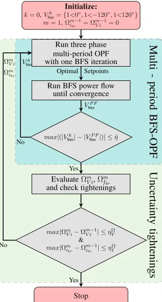
C. Solution Algorithm
In this section, we summarize the proposed solution method for the centralized CC-OPF scheme, sketched in Fig. 2. First, the initialization stage sets the uncertainty margins to zero and initializes the voltage levels of the three phases to a flat voltage profile. At the core of the proposed methodology lies the formulation of the three-phase multi-period centralized CC-OPF, which is summarized as
min u Nhor X t=1 X
z∈{a,b,c} Nb
X
j=1
CP·Pcurt,j,z,t+CQ·Qctrl,j,z,t
+ X
z∈{a,b,c} Nbr
X
i=1
CP·Ploss,i,z,t
·∆t
+CH·
||ηV||∞+||ηI||∞+||ηVUF||∞
(14)
subject to
Pinj,j,z,t=Pg,j,z,t−Plflex,j,z,t−(P ch B,j,z,t−P
dis B,j,z,t)
Qinj,j,z,t=Qg,j,z,t−Plflex,j,z,t·tan(φload) +QB,j,z,t
Iinj,j,z,t=
(Pinj,j,z,t+jQinj,j,z,t)∗ ¯
V∗ j,z,t
!
Ibr,t=BI BC·Iinj,t
∆Vt=BCBV ·Ibr,t Vt=Vslack−∆Vtap·ρt+ ∆Vt
ρmin≤ρt≤ρmax
|V-,j,t| ≤V U FMAX+ηVUF,j,t, ηVUF,j,t≥0
Pg,j,z,tmin ≤Pg,j,z,t≤P max g,j,z,t
Qmin
g,j,z,t≤Qg,j,z,t≤Q max g,j,z,t
Plflex,j,z,t=Pl,j,z,t+nj,z,t·Pshift,j,z,
Nhor
X
t=1
nj,z,t= 0
SoCbat min·E
bat cap,j,z≤E
bat j,z,t≤SoC
bat max·E
bat cap,j,z
Ebat
j,z,1=Estart
Ebat j,z,t=E
bat
j,z,t-1+ (ηbat·PB,j,z,tch −
Pdis B,j,z,t
ηbat )·∆t
0≤Pch B,j,z,t≤P
bat
max, 0≤P dis B,j,z,t≤P
bat max
Pch B,j,z,t+P
dis
B,j,z,t ≤max(P ch B,j,z,t, P
dis B,j,z,t)
Q2B,j,z,t≤(S bat
max)2−max((P ch B,j,z,t)2,(P
dis B,j,z,t)2) (
|RVj,z,t| ≤Vmax−Ω upper
V j,z,t+ηV,j,z,t
Re{RVj,z,t} ≥Vmin+ ΩlowerV j,z,t−ηV,j,z,t |Ibr,i,z,t| ≤Ii,z,max−ΩIbr,i+ηI,i,z,t.
Initialize: k= 0,Vk
bus={1<0◦,1<−120◦,1<120◦}
m= 1,Ωm−1
ibr = Ωm−1V i = 0
Run three phase multi-period OPF with one BFS iteration
Run BFS power flow until convergence
max|(|Vk bus| − |V
P F bus|)| ≤η˜
EvaluateΩm V i,Ω
m Ibr
and check tightenings
max|Ωm
V i−Ωm−1V i | ≤ηVΩ
& max|Ωm
ibr−Ωm−1ibr | ≤ηΩI
Stop
Yes No
Yes No
Multi
-period
BFS-OPF
Uncertainty
tightenings
Optimal Setpoints
VP F bus
Vk bus Ωm
[image:7.612.96.255.55.352.2]V i Ωm ibr
Fig. 2. Proposed centralized CC-OPF scheme for the computation of the optimal DER setpoints.
uncertainty loop bym. The iterative procedure continues until all parts of the algorithm have reached convergence.
The convergence characteristics of the proposed method are analyzed in [25], [32]. In [25], we show that the algorithm works well for practical cases where the OPF solution does not change significantly, i.e. does not show sudden changes from iteration to iteration. In this case, the tightenings do not change much, and convergence is reached after a few iterations. However, there might be cases where the algorithm does not converge. As explained in [32], subsequent iterates in the algorithm might cycle between repeated points that have large differences in the associated tightenings. In that paper, the authors followed a cut-and-branch approach to interrupt the cycling and enforce convergence. In our case, when we are faced with non-convergent cases, the algorithm uses an acceleration factor changing the solution less aggressively to avoid oscillations between repeated points, but at the cost of increasing the needed number of iterations.
III. OPTIMIZED LOCAL CONTROL DESIGN
In this section, we describe the core idea of the paper as summarized in Fig. 1. First, we discuss what kind of data are needed to perform the offline CC-OPF, which is explained in detail in Section II-A. Then, after deriving the optimal DER setpoints, we explain how we design the individual local controls for each DER using various ML techniques.
A. Optimal DER setpoint data generation
The first step is to generate the optimal DER setpoint data that will be used for the training of the local controls. To
do this, several operating scenarios are selected from seasonal historical data. Then, the CC-OPF of Section II is used to compute off-linethe optimal DER setpoints. The selection of the scenarios is critical, since they will form the basis for the training of the local schemes.
The DSO does not know the exact generation of all PVs in the LV system in the operational stage (as this would require detailed monitoring of all PVs). However, the DSO is aware of the installed DG capacity and the PV generation can be estimated with some uncertainty, using historical expected PV injection data and the installed capacity. These estimates are used in the CC-OPF solution.
The proposed method can be used with different seasonal data to account for seasonalities in terms of the DG injections and load. By changing the local control schemes based on the season, e.g. using the actual date, or when the topology of the DN changes, one can easily derive a behavior close to the optimal during the whole year.
B. Derivation of DG local controls
For the DGs, we derive optimized local controls for Active Power Curtailment (APC) and Reactive Power Control (RPC). These controls take the form of simple, piece-wise linear char-acteristic curves (such as in [18]), much like the local control schemes used today in industry. Unlike the current industry standards, these characteristics might have an arbitrarily large number of piece-wise linear segments and are optimized for each individual DG and DN.
Defining the location of the break-points and the slope coefficients is a non-linear and non-differentiable problem. Thus, we employ the method in Algorithm 1 coming from [37] that iteratively refines the location of the break-points while solving a constraint residual sum-of-squares (RSS) optimiza-tion problem for the slope coefficients.
Algorithm 1 Local DG control design (x∈ {p, q})
Input:Optimal DG setpoints
Output: Optimized local characteristic curve
1: Setns, initialize the break-pointss,i= 1,RSS0= 1000
2: Iterate:
RSSi:= min
˜
x0,β,s,γ T X
t
Pg,t·(xt−x˜t)2+ ns
X
k=1 γ2
k
subject to
˜
xt= ˜x0+β0·vt+ ns
P k=1
βk·(vt−sik)·I(vt>sik) +
− Pns k=1
γk·I(vt>sik)
Monotonicity and slope constraints
3: Update si+1
k = γk
βk +s
i
k and iteration indexi=i+ 1 4: Until: |RSSi−RSSi-1|<0.0001
5: Post-process the derived characteristic curves to be com-plete for all voltage values.
Return: Break-points s and slope factorsβ for each DG as
First, we define the number of break-pointsnsand initialize
them. Then, we use the iterative steps 2−4, where we solve the residual sum of squares problem using the active power injections as weights in the objective function, fitting the linear equivalent estimation model taking into account monotonicity and slope constraints. As inputs, we use the voltage vt for
each sample t, ∀t = 1, . . . , T. Then, we fit the linear model based on the known breakpoints si
k, ∀k = 1, . . . , ns at the
current iteration i, the left slope β0 and difference-in-slopes βk. The indicator functionI(·)becomes one when the inside
statement is true. Finally, x˜0 is the model intercept and γ a parameter which updates the location of the breakpoints towards the optimal one.
Omitting the indices for clarity, the key idea is to substitute the non-linear function β ·(v−s)·I(v > s) where both the difference-in-slope and the break-points are unknown, with its Taylor expansion using fixed break-points at each iteration i β·(v−si)·I(v >si)−γ·I(v >si)[37].
The same method is used both for the APC and RPC curves, using respectively the PV optimal active (p) and reactive (q) setpoints from the CC-OPF.
C. Local control of Battery Energy Storage Systems
Due to the more complex behavior of BESSs, e.g. inter-temporal constraints, we chose an SVM regression model to approximate the optimal setpoints of active and reactive power for the BESSs. An SVM regression model calculates a function, which deviates from the training data by a value no greater than a predetermined margin (ǫ in Algorithm 2), and at the same time is as flat as possible. SVM models are very powerful because they can also model nonlinear functions (or decision boundaries). This is achieved, by mapping the training set from the input space into higher dimensional spaces, called feature spaces, by performing a non-linear transformation using suitably chosen basis functions (kernels). Then, they solve the linear model in the new space problem, which describes a nonlinear behavior in the original (input) space [38]. The procedure of training the SVM controllers follows [19] and is summarized in Algorithm 2. We use as features (Φ) the local active and reactive power demand (Pload, Qload), the active power injection of the PV at the same
Algorithm 2 Local BESS control design (x∈ {p, q})
Input:Optimal BESS setpoints
Output: SVM model for the real-time BESS response
1: For each BESS unit form Φ = [V, Pload, Qload, Pg] and
assume a functionf(Φ) =
w,Φ +b.
2: Apply the linear, polynomial and radial-basis function kernels toΦ.
Solve: min w,b,ξ
1
2wTw+C
T P t=1
(ξ+ξ∗)
subject to x−
w,Φi
−b≤ǫ+ξ,∀ (Φi, x)
w,Φi
+b−x≤ǫ+ξ∗,∀ (Φi, x)
3: Identify the kernel with the lowest out-of-sample error
Return: {P, Q}B=f(V, Pload, Qload, Pg)
node (Pg) and the local voltage measurement (V). We then use
these local features, in their actual or a higher dimensional space through Kernels, to create a model that mimics the optimal response by the CC-OPF setpoints.
In order to derive the best SVM model, we test three different Kernels: the linear (
Φ,ΦT
in which case C in the objective function is a free parameter), the polynomial ((γ
Φ,ΦT
+r)d where C and the polynomial order d are
free parameters) and the Radial-Basis Function (RBF) Kernel (e(−γ|Φ−ΦT|)2
whereCand the kernel scaleγare free param-eters). Assuming a regression function f(Φ) =
w,Φ +b, we solve the convex optimization problem shown in Step 2, for all these Kernels in order to identify the most suitable one. The constantC, also called box constraint, takes positive values and penalizes the observations that lie outside the region defined by ǫ, helping to prevent overfitting (regularization). The value ofC assesses the trade-off between the flatness of the regression function and the amount up to which deviations larger than ǫ are tolerated. Finally, we keep the model with the kernel resulting in the lowest overall out-of-sample error through a 5-fold cross validation process.
D. Local control of Controllable Loads
For the controllable loads, we use an SVM model as a classifier, where we define three classes yc ∈ {−1,0,1} for
the ‘load decrease’, ‘no shifting’ and ‘load increase’ cases, respectively. As features we use Φ = [V, Pg], where V
is the local voltage measurement and Pg the active power
injection of the PV at the same node. Intuitively, high PV injections increase local voltages triggering a load increase action. The optimization problem is similar to the BESS case, withG(Φ) =sign(f(Φ)) being the classifier.
SVMs are able to deal with datasets with imbalanced class observations. This can be done by assigning different values for the box constraint (constantC) for ‘positive and ‘negative classes, i.e. changing the misclassification penalty for each class. This is equivalent to changing the class observation frequencies, i.e. oversampling the minority class. For example, ifCpos= 2·Cneg this is in principle equivalent to training a
standard SVM with C =Cneg after considering the positive
training samples twice. Such an approach implementing the so-called class-weighted SVM has been introduced in many references such as [39]. In our model, the classes of ‘load increase’ and ‘load decrease’ are balanced by design, due to constraints (9), that impose preservation of the daily load. Thus, since only the class no load shifting can comprise different amount of observation samples, we considered a different weight in this classification class.
IV. CASESTUDY- RESULTS
To analyze the performance of the proposed control design algorithm, we use a typical European radial LV grid [21], sketched in Fig. 3. The neutral is assumed to be earthed in several points, and due to the short lengths of cables the capacitance is neglected. The pole grounding impedance is
1 2
3 4 5 6 7 8 9 10 11
12 17 19
13
14 15 16
18
LV
[image:9.612.316.564.48.178.2]a,b,c
Fig. 3. Typical residential European LV grid [21].
effect of the ground return path is considered in the primitive impedance matrices. The interested reader is referred to [23] for modeling details.
The load and PV panels are distributed to the three phases unevenly, in order to simulate unbalanced conditions. More specifically, the total load taken from [21] is shared25%-60%
-15%among the three phases. The installed PV capacity, is set to SPV
rated = 150% of the total maximum load of the entire
feeder to the PV nodes= [3,5,7,10,12,16,17,18,19], and is shared 25%-25%-50% among the three phases.
Furthermore, a BESS is located on node 19 of phase C with capacity 12SPV
rated kWh, whereS PV
rated is the rated power of
the PV unit at that particular node. A flexible load of 5 kW connected to phase C of Node 16, whose total daily energy consumption needs to be constant. Please note that we assume single-phase connections for both the loads and the PV panels. For comparison, we perform three different investigations for the operation of the system:
• Method 0: The DGs are operating according to the
German grid-code rules [30], and no other DERs are allowed to be controlled by the DSOs. This corresponds to the current practice in industry.
• Method 1: All DERs are controlled based on the OPF-based algorithm described in Section II assuming perfect communication and monitoring infrastructure. As this serves as the benchmark of the best achievable perfor-mance, we consider perfect measurements and predictions for the whole time horizon without any uncertainty.
• Method 2: All DERs are operating according to the
individual controls derived in Section III.
The implementation was done in MATLAB. For the cen-tralized OPF-based control, YALMIP [40] was used as the modeling layer and Gurobi [41] as the solver. The results were obtained on an Intel Core i7-2600 CPU and 16 GB of RAM.
A. Derived local control
To derive the local control schemes of all DERs, we use a 30-day summer dataset with forecasts of the PV production with 1-hour time resolution. Thus, for all cases, the training set comprises 30∗24 = 7200 samples. Then, the algorithm described in Section II is used to generate the optimal DER setpoint data. The operational costs are assumed to be CP= 0.1CHF
kWh andCQ= 0.01·CP. The BESS, CL, and OLTC costs
are considered in the planning stage [20] and their use does not incur any operational cost to the DSO. Finally,CH= 1000·CP
is used to avoid infeasible solutions. For the CC-OPF, we
0
.
85
0
.
9
0
.
95
1
1
.
05
1
.
1
−
1
−
0
.
5
0
0
.
5
1
Voltage magnitude (p.u.)
Q
g/Q
m
a
x
(p
.u
.)
PV 3 PV 5 PV 7 PV 10 PV 12
PV 16 PV 17 PV 18 PV 19
Fig. 4. Individual local characteristic curves for reactive power control of the PV units at phase C.
use forecast error distributions from [42], and draw 1000
samples from the 9-hour ahead forecast error distribution of the summer power profiles similar to [25]. We assume a perfect spatial correlation, implying that all PVs follow the same distribution. An acceptable violation probability of ǫ= 5%is used. Then, from the generated optimal DER setpoint data, we derive the local controls as described in Section III. Figure 4 shows the individual local characteristic curves derived with Algorithm 1 for the RPC of the PV units in phase C. It can be seen that the units closer to the secondary of the substation, i.e. 3, 5 and 12 show a capacitive behavior optimizing the losses, while the ones facing overvoltage problems at the end of the feeder, e.g. 16and 19, show an inductive behavior at smaller voltages than the maximum of1.04p.u.
To obtain BESS and controllable load models that behave well on unseen data, we perform cross-validation (or out-of-sample testing), which is a re-sampling procedure to test the models performance on new data. This procedure helps identifying overfitting or selection bias issues and to provide intuition on how the model generalizes to an independent dataset. In both SVM models, we followed a 5-fold cross-validation procedure, partitioning the sample data into 5 sets of 144 samples. We train the SVM models using 4 folds, and use the remaining to measure the performance. Finally, after combining (averaging) the results of multiple rounds of
0.98 0.99 1 1.01 1.02 1.03
0
0.2
0.4
0.6
0.8
1
Voltage magnitude (p.u.)
Lo
cal
PV
injection
(p.u.)
[image:9.612.62.290.62.162.2]no load shifting load decrease load increase
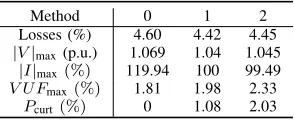
[image:9.612.315.557.534.713.2]TABLE I
SUMMARIZED MONTHLY RESULTS FOR ALL METHODS(ONLY THE
LARGEST OBSERVED VALUE IS LISTED)
Method 0 1 2
Losses (%) 4.60 4.42 4.45
|V|max(p.u.) 1.069 1.04 1.045
|I|max(%) 119.94 100 99.49
V U Fmax(%) 1.81 1.98 2.33
Pcurt(%) 0 1.08 2.03
cross-validation, we derive a more accurate estimate of model prediction performance. For the BESS models, derived with Algorithm 2, the RBF kernel functions resulted in the best behavior in terms of out-of-sample validation procedure with the following parameters: constant C = 236.78, ǫ= 0.0025, γ= 1.12, showing an overallRM SEof 0.158.
Finally, for the controllable loads, the method detailed in Section III-D gives a classifier with overall accuracy of
100%since the data are perfectly linearly separable. Figure 5 shows the decision boundaries that define the three classes in the space of the two features. As can be observed, for PV injections higher than 0.3 p.u. the load is increased to reduce the local voltage in combination with the other available measures. In low PV injections, e.g. during evening hours, the load is decreased to maintain the total daily demand constant, or is not shifted.
[image:10.612.102.249.85.145.2]B. Results
Table I summarizes the results from applying the three methods in real-time operation for a test period of one month. Method 1 corresponds to the benchmark as it satisfies all security constraints and minimizes the objective function. Method 0 (standard industry practice) results in higher losses than the OPF-based approach, due to increased needs for re-active power by the PV units, without solving the overvoltage, overload, or balancing issues. Finally, Method 2 mitigates adequately the overvoltages and overloads to values acceptable by grid codes, while being capable of mimicking the OPF-based control without the need of communication. Moreover, it significantly improves the balancing problems with only small violations during 5 hours in the month, which is also acceptable as defined by the grid codes. Figure 6 displays the real-time control behaviour of the BESS and PV unit at Node 19, phase C, operating according to Methods 1 and 2. It can be seen that the proposed local control (Method 2) of the BESS and PV is more conservative than the OPF-based approach (Method1) where the PV unit absorbs the maximum reactive power for most voltage levels due to the overvoltage problems. This conservative behavior is due to the CC-OPF approach we employ (Section II) to generate the data used for deriving the controls of Method 2. On the contrary, the OPF-based control (Method 1) uses the actual data, assuming full knowledge of the network, load and production values through an ideal communication system without delays. Despite this, the response using the proposed local controls mimics the OPF response in a satisfactory way.
Finally, Fig. 7 shows the evolution of the voltage at Node 19 over the ten days. It can be seen that operating with the current regulations (Method0) leads to frequent overvoltages.
Fig. 6. Real-time control schemes of the BESS and PV unit of Node 19 phase C.
24 48 72 96 120 144 168 192 216 240 1
1.02 1.04 1.06
Time (h)
V
ol
tage
(p
.u
.)
[image:10.612.319.555.266.399.2]0 1 2 Vmax
Fig. 7. Voltage magnitude evolution at phase C of Node 19.
24 48 72 96 120 144 168 192 216 240 0
50 100
Time (h)
T
h
er
m
al
load
in
g
(%
)
0 1 2 |I|maxFig. 8. Current magnitude evolution at phase C of Cable 2–3
On the contrary, the OPF-based approach (Method1) and the proposed local control satisfy the voltage security constraints. Similar observations can be made for the thermal loading, shown for Cable 2–3 in Fig. 8.
V. CONCLUSION
[image:10.612.316.555.423.541.2]In this paper, we propose a data-driven local control design methodology to derive local DER controls that can mimic the centralized controller optimal behavior, without the need for monitoring and communication infrastructure. This is based on using ML techniques to derive optimized local controls based on historical data processed through a CC-OPF. The controllers are simple to compute, understand, and implement. Yet, we have shown through the examples used that the proposed local controls can tackle security problems in an un-balanced and challenging environment while at the same time optimize its operation. Future work will focus on comparing data-driven control schemes using other ML techniques, and subsequently, on assessing risks and challenges of using such schemes at operating conditions, which were not seen in the training dataset.
REFERENCES
[1] N. Hatziargyriou, O. Vlachokyriakou, T. Van Cutsem, J. Milanovi´c, P. Pourbeik, C. Vournas, M. Hong, R. Ramos, J. Boemer, P. Aristidou, V. Singhvi, J. dos Santos, and L. Colombari, “Task Force on Contribution to Bulk System Control and Stability by Distributed Energy Resources connected at Distribution Network,” IEEE PES, Tech. Rep., 2017. [2] P. Fortenbacher, M. Zellner, and G. Andersson, “Optimal sizing and
placement of distributed storage in low voltage networks,” in Pro-ceedings of the 19th Power Systems Computation Conference (PSCC), Genova, Jun 2016.
[3] S. Karagiannopoulos, P. Aristidou, A. Ulbig, S. Koch, and G. Hug, “Op-timal planning of distribution grids considering active power curtailment and reactive power control,”IEEE PES General Meeting, 2016. [4] J. Lavaei and S. H. Low, “Zero duality gap in optimal power flow
problem,” IEEE Transactions on Power Systems, vol. 27, no. 1, pp. 92–107, 2012.
[5] D. K. Molzahn and I. A. Hiskens, “Sparsity-Exploiting Moment-Based Relaxations of the Optimal Power Flow Problem,”IEEE Transactions on Power Systems, vol. 30, no. 6, pp. 3168–3180, Nov 2015. [6] D. K. Molzahn, B. C. Lesieutre, and C. L. DeMarco, “Investigation
of Non-zero Duality Gap Solutions to a Semidefinite Relaxation of the Optimal Power Flow Problem,” in2014 47th Hawaii International Conference on System Sciences. IEEE, jan 2014, pp. 2325–2334. [7] A. S. Zamzam, N. D. Sidiropoulos, and E. Dall’Anese, “Beyond
Relax-ation and NewtonRaphson: Solving AC OPF for Multi-Phase Systems With Renewables,”IEEE Transactions on Smart Grid, vol. 9, no. 5, pp. 3966–3975, Sep 2018.
[8] S. Bolognani and F. D¨orfler, “Fast power system analysis via implicit linearization of the power flow manifold,” inProc. 53rd Annual Allerton Conference on Communication, Control, and Computing, 2015. [9] R. Tonkoski, L. A. C. Lopes, and T. H. M. El-Fouly, “Coordinated
active power curtailment of grid connected PV inverters for overvoltage prevention,”IEEE Transactions on Sustainable Energy, vol. 2, no. 2, pp. 139–147, 2011.
[10] P. Kotsampopoulos, N. Hatziargyriou, B. Bletterie, and G. Lauss, “Review, analysis and recommendations on recent guidelines for the provision of ancillary services by Distributed Generation,” in IEEE IWIES, 2013, pp. 185–190.
[11] S. Bolognani and S. Zampieri, “A distributed control strategy for reactive power compensation in smart microgrids,”IEEE Transactions on Automatic Control, vol. 58, no. 11, pp. 2818–2833, Nov. 2013. [12] F. Olivier, P. Aristidou, D. Ernst, and T. V. Cutsem, “Active management
of low-voltage networks for mitigating overvoltages due to photovoltaic units,”IEEE Transactions on Smart Grid, vol. 7, no. 2, pp. 926–936, March 2016.
[13] Y. Guo, K. Baker, E. Dall’Anese, Z. Hu, and T. Summers, “Data-based distributionally robust stochastic optimal power flow, Part I: Methodologies,”IEEE Transactions on Power Systems, 2018. [14] ——, “Data-based distributionally robust stochastic optimal power flow,
Part II: Case studies,”IEEE Transactions on Power Systems, 2018. [15] A. Garg, M. Jalali, V. Kekatos, and N. Gatsis, “Kernel-Based
Learning for Smart Inverter Control,” July 2018. [Online]. Available: https://arxiv.org/pdf/1807.03769.pdf
[16] R. Dobbe, O. Sondermeijer, D. Fridovich-Keil, D. Arnold, D. Callaway, and C. Tomlin, “Data-Driven Decentralized Optimal Power Flow,” 2018. [Online]. Available: http://arxiv.org/abs/1806.06790
[17] O. Sondermeijer, R. Dobbe, D. Arnold, and C. Tomlin, “Regression-based Inverter Control for Decentralized Optimal Power Flow and Voltage Regulation,”IEEE PES General Meeting, 2016.
[18] S. Karagiannopoulos, P. Aristidou, and G. Hug, “Hybrid approach for planning and operating active distribution grids,”IET Generation, Transmission & Distribution, pp. 685–695, Feb 2017.
[19] F. Bellizio, S. Karagiannopoulos, P. Aristidou, and G. Hug, “Optimized local control schemes for active distribution grids using machine learning techniques,” inIEEE PES General Meeting, June 2018.
[20] S. Karagiannopoulos, P. Aristidou, and G. Hug, “Co-optimisation of Planning and Operation for Active Distribution Grids,” inProceedings of the 12th IEEE Power and Energy Society PowerTech Conference, Manchester, Jun 2017.
[21] K. Strunz, E. Abbasi, C. Abbey, C. Andrieu, F. Gao, T. Gaunt, A. Gole, N. Hatziargyriou, and R. Iravani, “Benchmark Systems for Network Integration of Renewable and Distributed Energy Resources,”CIGRE, Task Force C6.04, no. 273, pp. 4–6, 4 2014.
[22] L. Ochoa, R. Ciric, A. Padilha-Feltrin, and G. Harrison, “Evaluation of distribution system losses due to load unbalance,” Power Systems Computation Conference, Li`ege, Belgium, 2005, vol. 5, no. August, p. 4, Nov 2005.
[23] W. H. Kersting,Distribution System Modeling and Analysis, 2002. [24] J. H. Teng, “A direct approach for distribution system load flow
solutions,”IEEE Transactions on Power Delivery, vol. 18, no. 3, pp. 882–887, 2003.
[25] S. Karagiannopoulos, P. Aristidou, L. Roald, and G. Hug, “Operational Planning of Active Distribution Grids under Uncertainty,” inIREP 2017, X Bulk Power Systems Dynamics and Control Symposium, Aug 2017. [26] S. Karagiannopoulos, P. Aristidou, and G. Hug, “A Centralised Control
Method for Tackling Unbalances in Active Distribution Grids,” in
in Proceedings of the 20th Power Systems Computation Conference (PSCC), Dublin, June 2018.
[27] P. Pillay and M. Manyage, “Definitions of Voltage Unbalance,”IEEE Power Engineering Review, vol. 21, no. 5, pp. 49–51, 2001.
[28] IEC 61000-3-14:, “Electromagnetic compatibility (EMC) - Part 3-14: Assessment of emission limits for harmonics, interharmonics, voltage fluctuations and unbalance for the connection of disturbing installations to LV power systems.” Tech. Rep., 2011.
[29] EN 50160, “Standard EN 50160, voltage characteristics of electricity supplied by public electricity networks,” 2010.
[30] VDE-AR-N 4105, “Power generation systems connected to the LV distribution network.” FNN, Tech. Rep., 2011.
[31] D. Bienstock, M. Chertkov, and S. Harnett, “Chance-Constrained Op-timal Power Flow: Risk-Aware Network Control under Uncertainty,”
SIAM Review, vol. 56, no. 3, pp. 461–495, Jan. 2014.
[32] L. A. Roald, D. K. Molzahn, and A. F. Tobler, “Power System Opti-mization with Uncertainty and AC Power Flow: Analysis of an Iterative Algorithm,” inIREP 2017, X Bulk Power Systems Dynamics and Control Symposium, Aug 2017.
[33] L. Roald, F. Oldewurtel, B. Van Parys, and G. Andersson, “Security Constrained Optimal Power Flow with Distributionally Robust Chance Constraints,” aug 2015. [Online]. Available: http://arxiv.org/abs/1508.06061
[34] L. Roald, F. Oldewurtel, T. Krause, and G. Andersson, “Analytical refor-mulation of security constrained optimal power flow with probabilistic constraints,” inProceedings of the 10th IEEE Power and Energy Society PowerTech Conference, Grenoble, Jun 2013.
[35] L. Roald and G. Andersson, “Chance-Constrained AC Optimal Power Flow: Reformulations and Efficient Algorithms,” Jun. 2017. [Online]. Available: https://arxiv.org/abs/1706.03241
[36] J. Schmidli, L. Roald, S. Chatzivasileiadis, and G. Andersson, “Stochas-tic AC optimal power flow with approximate chance-constraints,” in
IEEE Power and Energy Society General Meeting (PESGM), Jul 2016. [37] V. M. R. Muggeo, “Estimating regression models with unknown break-points,”Statistics in Medicine, vol. 22, no. 19, pp. 3055–3071, oct 2003. [38] T. Hastie, R. Tibshirani, and J. Friedman, The elements of statistical
learning: data mining, inference and prediction. Springer, 2009. [39] E. E. Osuna, R. Freund, and F. Girosi, “Support Vector Machines :
Training and Applications,”MIT, vol. 9217041, no. 1602, 1997. [40] J. L¨ofberg, “Yalmip : A toolbox for modeling and optimization in
matlab,” inIn Proceedings of the CACSD Conference, Taiwan, 2004. [41] I. Gurobi Optimization, “Gurobi optimizer reference manual,” 2016.
[Online]. Available: http://www.gurobi.com
Stavros Karagiannopoulos (S’15) was born in Thessaloniki, Greece. He received a Diploma in Electrical and Computer Engineering from the Aris-totle University of Thessaloniki, Greece, in 2010, and a M.Sc. degree in Energy Science and Technol-ogy from the Swiss Federal Institute of TechnolTechnol-ogy (ETH), Zurich, Switzerland, in 2013. After that, he worked at ABB Corporate Research Center in Switzerland, and since 2015, he has been pursuing the Ph.D. degree with the Power Systems Labora-tory, ETH Zurich, Zurich, Switzerland. His main research focuses on planning and operation of active distribution grids.
Petros Aristidou(S’10-M’15) received a Diploma in Electrical and Computer Engineering from the National Technical University of Athens, Greece, in 2010, and a Ph.D. in Engineering Sciences from the University of Li`ege, Belgium, in 2015. He is currently a Lecturer (Assistant Professor) in Smart Energy Systems at the University of Leeds, U.K. His research interests include power system dynamics, control, and simulation.

![Fig. 3. Typical residential European LV grid [21].](https://thumb-us.123doks.com/thumbv2/123dok_us/1863254.143232/9.612.315.557.534.713/fig-typical-residential-european-lv-grid.webp)