City, University of London Institutional Repository
Citation
:
Turkay, C., Kaya, E., Balcisoy, S. and Hauser, H. (2017). Designing Progressive
and Interactive Analytics Processes for High-Dimensional Data Analysis. IEEE Transactions
on Visualization and Computer Graphics, 23(1), pp. 131-140. doi:
10.1109/TVCG.2016.2598470
This is the accepted version of the paper.
This version of the publication may differ from the final published
version.
Permanent repository link:
http://openaccess.city.ac.uk/15205/
Link to published version
:
http://dx.doi.org/10.1109/TVCG.2016.2598470
Copyright and reuse:
City Research Online aims to make research
outputs of City, University of London available to a wider audience.
Copyright and Moral Rights remain with the author(s) and/or copyright
holders. URLs from City Research Online may be freely distributed and
linked to.
Supplementary Material for:
“Designing Progressive and Interactive Analytics Processes for
High-Dimensional Data Analysis”
Cagatay Turkay, Erdem Kaya, Selim Balcisoy, Helwig Hauser
1 CASESTUDY
1.1 Dataset
The data analyzed during the case study comprises credit card transaction features, customer demographics and financial metrics, and normalized features.
1.1.1 Credit Card Transaction Features
• cust idCustomer ID
• tx dateTransaction Date
• tx timeTransaction Time
• tx amountTransaction Amount
• merch typeMerchant Type (MMC Code)
• merch idAnonymized Merchant ID
• online txOnline Transaction Flag (True or False)
• exp typeExpenditure Type
• currencyCurrency
• pos xLongitude of the Transaction Location
• pos yLatitude of the Transaction Location
1.1.2 Customer Demographic and Financial Metrics
• marital statMarital status of the customer making the transaction
• edu statEducational status of the customer making the transaction
• job typeThe category of the job of the customer making the transaction
• incomeMonthly income of the customer making the transaction
• ageAge of the customer making the transaction
• bank ageThe number years spent as a customer of the bank of the customer making the transaction
• cc mean riskA score showing how risky the customer is from the bank’s perspective
• total num ccTotal number of the credit cards owned by the customer making the transaction
• other total num ccTotal number of credit cards issued by other banks and owned by the customer making the transaction
• bank cc max limitThe maximum credit card limit given to the customer by the bank during the data collection period
• all cc max limitThe maximum credit card limit given to the customer by all banks during the data collection period
• total transferThe total within-bank wired transfer made by the customer making the transaction during the data collection period.
• mean transferThe mean within-bank wired transfer amount made by the customer making the transaction during the data collection period
• mean eftThe total within-bank wired transfer made by the customer making the transaction during the data collection period
• total eftThe total between-banks EFT (Electronic Funds Transfer) amount made by the customer making the transaction during the data collection period
• eft entropyA measure of the customer showing his/her diversity in issuing EFT to other banks. Higher value indicates that the customer distributed his/her EFT transfers evenly over the banks to which he/she performed an EFT transfer.
• total atm withdrawalThe total amount of the ATM withdrawals made by the customer throughout the data collection period.
• total atm depositThe total amount of the ATM deposits made by the customer throughout the data collection period.
• accept percentThe rate of the total number of acceptance of the customers for various offerings made by the bank to the number of total offerings.
• resp score meanThe average response score of the customers, calculated by the bank, indicating the responsiveness of the customers with respect to any interactions initiated by the bank.
• resp score stddevThe standard deviation of the response scores of the customers calculated by the bank.
• risk score meanThe average risk score of the customers, calculated by the bank.
• mobile total transferThe total within-bank wired transfer made by the customer over mobile application during the data collection period.
• mobile total eftThe total between-banks EFT amount made by the customer over the mobile application during the data collection period.
• mean expThe average credit card expenditures of the customer over the data collection period.
• total expThe total credit card expenditures of the customer over the data collection period.
1.1.3 Normalized Features
• tx amount nThe linear mapping of the tx amount feature to the range [0,1].
• income nThe linear mapping of the income feature to the range [0,1].
• age nThe linear mapping of the age feature to the range [0,1].
• bank age nThe linear mapping of the bank age feature to the range [0,1].
• total num cc nThe linear mapping of the total num cc feature to the range [0,1].
• bank cc max limit nThe linear mapping of the bank cc max limit feature to the range [0,1].
• all cc max limit nThe linear mapping of the all cc max limit feature to the range [0,1].
• total transfer nThe linear mapping of the total transfer feature to the range [0,1].
• mean transfer nThe linear mapping of the mean transfer feature to the range [0,1].
• mean eft nThe linear mapping of the mean eft feature to the range [0,1].
• total eft nThe linear mapping of the total eft feature to the range [0,1].
• total atm withdrawal nThe linear mapping of the total atm withdrawal feature to the range [0,1].
• total atm deposit nThe linear mapping of the total atm deposit feature to the range [0,1].
• mobile total transfer nThe linear mapping of the mobile total transfer feature to the range [0,1].
• mobile total eft nThe linear mapping of the mobile total eft feature to the range [0,1].
• mean exp nThe linear mapping of the mean exp feature to the range [0,1].
• total exp nThe linear mapping of the total exp feature to the range [0,1].
1.1.4 Data Pruning
The data has been pruned in order to prevent various kinds of distortions in the visualizations such as stacking of data points to a relatively small area due to extremely high-valued points. The data has been pruned with respect to conditions listed below. For any condition, no more than 0.5% of the data has been pruned. As a result of pruning process, approximately 4% of the data have been dropped.
All the transaction tuples satisfyingallof the following conditions formed the dataset used in the study.
• income<10000
• total transfer<1000000
• mean transfer<100000
• mean eft<100000
• total eft<1500000
• total atm withdrawal<80000
• total atm deposit<250000
• mobile total transfer<500000
• mobile total eft<800000
1.2 Tasks
The tasks and example workflow utilizing these tasks are discussed in detail in the paper. Below is the mapping between our high-level tasks and the task abstractions of Yi et al. [5].
Task # High-level Task Abstract Actions
Task-1 Automatic Feature-based Subsegment Generation selection, filtering, clustering, comparison Task-2 User-defined Subsegment Definition selection, filtering, clustering, comparison
Task-3 Segment Composition retrieve, reconfigure
Task-4 Segment Fine-tuning retrieve, filtering, comparison, selection
[image:4.612.112.508.103.182.2]Task-5 Composed Segment Description retrieve, elaborate
Table 1. Mapping between high-level tasks and abstract actions based on Yi et al.’s [5] taxonomy.
1.3 Selectable Features
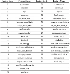
Selectable features in the difference view of the DimXplorer are listed in Table 1.3 and in “Normalized Features” subsection.
Feature Code Feature Name Feature Code Feature Name
1 tx amount 21 tx amount n
2 income 22 income n
3 age 23 age n
4 bank age 24 bank age n
5 cc mean risk 25 total num cc n
6 bank cc max limit 26 bank cc max limit n
7 all cc max limit 27 all cc max limit n
8 total transfer 28 total transfer n
9 mean transfer 29 mean transfer n
10 mean eft 30 mean eft n
11 total eft 31 total eft n
12 eft entropy 32 total atm withdrawal n
13 total atm withdrawal 33 total atm deposit n
14 total atm deposit 34 mobile total transfer n
15 accept percent 35 mobile total eft n
16 resp score mean 36 mean exp n
17 resp score stddev 37 total exp n
18 mobile total transfer
19 mean exp
[image:4.612.163.458.265.580.2]20 total exp
Table 2. Selectable features.
1.4 Feature Set Selection
The set of features selected by the analysts during the analysis sessions were recorded and represented in Table 3. Moment shows the time elapsed during the start of the corresponding sub-session until a feature set selection made by the analysts. Duration represents the time elapsed that the analysts spent on working on the selected feature set. The numbers in the feature set selection column are the index numbers of the features listed in Table 1.3. The progression below, recorded as multiples of 25, shows the maximum percentage of the whole data contributed to the calculations as of the moment the analysts renounced the selected feature set. Insights-Questions-Hypotheses column shows the total number of insights, questions, and hypotheses arose during the time period analysts worked with corresponding feature set.
Sub-session Moment Duration Feature Set Selection Progression Below Insights-Questions-Hypotheses
2-1 1:23 2:10 1,3,7 75 0-2-0
2-2 0:05 7:11 1,4,8 75 1-0-0
2-2 17:30 7:10 1,9 75 2-0-0
2-3 00:00 4:45 1,9 100 1-0-1
2-3 5:58 4:19 3,6 50 1-0-1
2-3 10:23 9:32 3,12,17,18 100 2-2-0
2-4 5:14 4:55 1,3 50 0-2-0
2-4 10:09 1:35 1,3,6,12 25 0-0-0
2-4 11:59 5:26 1,3,9,10,15 25 0-0-0
2-4 20:32 9:50 3,5,7 75 2-1-0
3-1 2:02 4:03 22,23,26 25 1-0-0
3-1 27:00 6:05 22,23,27,34,35 50 0-2-0
3-1 33:05 4:15 23,27,34,35 25 1-0-0
3-1 37:20 17:10 23,27,32,33 75 2-0-0
3-2 0:00 4:03 23,27,29,33 25 0-0-0
3-2 4:03 4:37 12,15,16,24,25 50 0-0-1
3-2 12:40 4:29 12,15,16,36 25 0-0-1
3-2 17:09 3:22 12,15,16,37 50 0-0-1
4-1 2:00 6:06 25,31,33 NP 0-0-1
4-1 10:42 8:53 12,15,26,36 NP 0-3-0
4-1 24:34 25:34 22,23,25 NP 0-0-0
4-1 25:34 11:35 22,23,25,26 NP 1-0-0
[image:5.612.51.557.350.749.2]4-2 19:03 11:54 25,32,33,36,37 NP 1-1-0
Table 3: Feature set selections performed by analysts during the course of the analysis sessions. NP stands for “non-progressive.”
1.5 Insights-Questions-Hypotheses
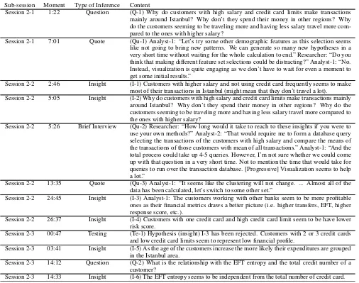
Important take-away points were extracted from the analysis video records and are listed as follows.
Sub-session Moment Type of Inference Content
Session 2-1 1:22 Question (Q-1) Why do customers with high salary and credit card limits make transactions mainly around Istanbul? Why don’t they spend their money in other regions? Why do the customers seeming to be traveling more and having less salary travel more com-pared to the ones with higher salary?
Session 2-1 7:01 Quote (Qu-1) Analyst-1: “Let’s try some other demographic features as this selection seems like not going to bring new patterns. We can generate so many new hypotheses in a very short time without waiting for the whole calculation to end.” Researcher: “Do you think that making different feature set selections could be distracting?” Analyst-1: “No. Instead, visualization is quite engaging as we don’t have to wait for even a moment to get some initial results.”
Session 2-2 2:46 Insight (I-1) Customers with higher salary and not using credit card frequently seems to make most of their transactions in Istanbul (might mean that they don’t travel a lot). Session 2-2 5:05 Insight (I-2) Why do customers with high salary and credit card limits make transactions mainly
around Istanbul? Why don’t they spend their money in other regions? Why do the customers seeming to be traveling more and having less salary travel more compared to the ones with higher salary?
Session 2-2 5:26 Brief Interview (Qu-2) Researcher: “How long would it take to reach to these insights if you were to use your own methods?” Analyst-2: “That would require me to form a database query selecting the transactions of the customers with high salary and compare the means of the transactions of those customers with mean of all transactions.” Analyst-1: “And the total process could take up 4-5 queries. However, I’m not sure whether we could come up with that question in a very short time. Not to mention the time that would take for queries to run over the transaction database. [Progressive] Visualization seems to help a lot.”
Session 2-2 13:35 Quote (Qu-3) Analyst-1: “It seems like the clustering will not change. ... Almost all of the data has been calculated, let’s switch to some other set.”
Session 2-2 24:45 Insight (I-3) Analyst-1: The customers working with other banks seem to be more profitable ones as their financial metrics draws a better picture (i.e. higher transfers, EFT, higher response score, etc.).
Session 2-2 26:37 Insight (I-4) Customers with one credit card and high credit card limit seem to be have lower risk score.
Session 2-3 00:47 Testing (Te-1) Hypothesis (insight) I-3 has been rejected. Customers with 2 or 3 credit cards and low credit card limits seem to represent low financial profile.
Session 2-3 03:41 Insight (I-5) As the age of the customers increase the more likely their expenditures are grouped in the Istanbul area.
Session 2-3 14:12 Question (Q-2) What is the relationship with the EFT entropy and the total credit number of a customer?
Session 2-3 15:49 Insight (I-7) Customers working with other banks seem to be managing their credit cards and their assets via those other banks, not via our bank. (Analyst-1)
Session 2-3 17:01 Question (Q-3) Why do customers having more than one credit card have lower EFT entropy? Session 2-4 5:17 Question (Q-4) Can the transaction amount and the age of the customer be a good discriminator
in terms of facilitating good segmentation? Can the transaction amount and the age of the customer be related to money deposit or withdrawal amount?
Session 2-4 11:24 Quote (Qu-4) Analyst-4 accidentally deleted all the selections including the features, which immediately stopped all ongoing clustering and PCA calculations. Analyst-3: “Sigh, all the computations have gone.” Analyst-1 “No worries. Make the selection again, please. They (clusters) should show up soon.” However, after this dialog, they ended up starting with a slightly different feature set.
Session 2-4 12:06 Brief Interview (Qu-5) Researcher: “To what extend do you think this tool (progressive visual analytic system) can effect your current analysis processes?” Analyst-1: “Recently we changed our policy which could be summarized as ’work on old but important hypotheses’ to a stance encouraging our analyst teams for the production of new hypotheses. This ap-proach, I believe, can take us one step forward as we will be trying out new alternatives. It seems like this tool is a good fit, at least conceptually, as our analysis is now more data-driven rather than goal-driven. ... (16:03) It is quite a new concept for my team to have almost-real-time response from a clustering calculation. ... (17:09) Typically, given the usual dataset size and analysis goals, we spare more than a day for clustering a model.”
Session 2-4 21:18 Insight (I-8) There seems to be a positive correlation with the age and income of the customer. Session 2-4 25:47 Question (Q-5) Do the transactions mostly done close to coastal line of the city form a cluster
based on the feature set with age, mean risk and maximum credit card limit? Session 2-4 29:25 Insight (I-9) Online transactions seem to be clustered around the west half of the city. Session 3-1 2:12 Quote (Qu-6) Just after a new feature set has been selected, Analyst-3: “I think we can start as
we have a good view of the clusters.”
Session 3-1 3:10 Quote (Qu-7) The team tried a new set of features and immediately observed a ‘good’ sepa-ration of data points. However, after only 15-20 seconds, the sepasepa-ration dramatically changed. After this, Analyst-2: “Well, I think waiting for a while might be a good thing.”
Session 3-1 3:35 Insight (I-10) As expected, there is a correlation between the credit card limit and income. Session 3-1 27:29 Question (Q-6) Are the features age and income together predictor of credit card limit or total
transfer amount?
Session 3-1 30:02 Question (Q-7) How do the clusters differ from each other in terms of total transfer amount? Session 3-1 40:47 Insight (I-11) The number of the credit card of the customer and the amount of expenditures
made by him/her are not correlated.
Session 3-1 50:47 Observation (Qu-8) Analyst-3 started to pose his idea and requested one of his fellow analyst to modify a particular visualization parameter. As soon as he noticed that visualization was changing on the screen, he said: “Well, let’s wait for a moment to let it settle down.” They waited for a couple of seconds so that DimXplorer could processed some more data.
Session 3-1 51:03 Design Informant (Qu-9) During the course of the analysis, Analyst-3: “I’ve just seen a high response score for the selected cluster, but it has just gone away.” As the clustering algorithm con-tinued to its calculations, the relevant data points have moved to other clusters changing the pattern Analyst-3 previously discovered: “Wouldn’t it be nice to have a button that simply pauses the progressive visualization?”
Session 3-2 08:11 Hypothesis (H-1) The customers with low EFT entropy are also the ones with high response scores. Session 3-2 08:40 Technical Problem The analysis session has been paused. The session continued after approximately 4
minutes.
Session 3-2 14:59 Testing (Te-2) H-1 has been verified. Customers with high response scores were also the ones with low EFT entropy. The reverse was also true, as it was clear on the comparison with PCA and cluster views.
Session 3-2 20:31 Brief Interview (Qu-10) Researcher: “I have been observing that you are making quick and brief infer-ences from the data.” They were able to interactively try out many different filters and features for the clustering in a short time. Previously, they reported that these kind of changes would actually require a workday. “How do you think these brief findings can contribute to your actual analysis activities?” Analyst-3: “Well, we can further elabo-rate on the hypotheses that we derived from this tool. For example, we have seen that the customers with high EFT entropy tend to have low response scores. Well, we could verify this in more detail and, maybe, we can also investigate the outliers, the customers with high response scores and high EFT entropy, to find out why they discriminate from the majority.” Analyst-2: “For example, if they are not credit card customers, I would try to ‘get deep with them’ with credit card offers.” Analyst-3: “Moreover, if they make more EFT than they actually need, I would recommend them to apply for automatic payment services.” Analyst-4: “It could also help us to locate a customer group that we have never been aware of. In that case, we could devise new actions for that new particular group.”
Session 3-2 22:07 Brief Interview (Qu-11) Researcher: “How do you usually go about inferring hypotheses during your daily analysis activities?” Analyst-4: “Experience and limited visualizations usually form a basis for our hypotheses extraction processes.” Analyst-3: “Well, first of all, we couldn’t get all those results that quickly. As we get some results from our data analytic models, we become aware of even more other options that we feel like we need to try. Well, we don’t have that much time.” Analyst-2: “And this situation may lead to indolence, particularly when your models take so much time to be calculated.” Analyst-3: “And [when working on this tool] we are able to look at the model altogether which is way better than one person working on his own.” Analyst-4: “Due to time limitations, we regularly eliminate the minor or insignificant cases, but we are able try them here in a short time.” Research: “Aren’t there situations that you work on the models as a team?” Analyst-2: “Of course there are. For example, one of us develops a model and we brainstorm on it. However, we usually get the feeling that the analyst working on that model must have spent much time on it and we cannot easily give up and try new models. However, during study I noticed that we can reject our own models as quickly as we generate them. It is easy to reject them on this tool.” Analyst-4: “Analysis, especially exploratory one, is usually like a lottery, the more ticket you have, the more likely you win the prize. With this tool, we have many more tickets.”
Session 4-1 2:30 Injection DimXplorer has been configured to work in non-progressive mode. For any calculation, if the calculations are completed in less than 60 seconds, the DimXplorer will respond in at least 60 seconds.
Session 4-1 2:53 Observation During the delay (60 seconds) that was intentionally inserted to simulate non-progressive analytics, Analyst-4 started to talk about what they would be expecting at the end of the clustering calculation.
Session 4-1 2:58 Hypothesis (H-3) There is a positive correlation between EFT entropy and total number of credit cards per customer.
Session 4-1 12:17 Observation At the end of the NP clustering calculation they were satisfied with the result of the clustering; however, they noticed that they forgot to change the feature on the axes of cluster small multiples. Instead of having the result to be recalculated, they decided to continue to the analysis with the old view.
Session 4-1 17:17 Question (Q-8) How does the campaign acceptance rate of the customers change with high EFT entropy and high number of credit cards?
Session 4-1 17:36 Question (Q-9) There are customers with high EFT entropy but also falling into one of the sub-groups with high and low acceptance rate. What causes this discrimination?
Session 4-1 19:01 Question (Q-10) Is there a positive correlation between the credit card number and the credit card limit that was granted by our bank?
Session 4-1 22:29 Quote (Qu-12) Analyst-3: “I think it might also be beneficial to be able to set the step size of the progression. For example, it can be distracting to look at an ever-changing visual-ization. Can we follow a different approach, say, process a certain fraction of the data at each step of calculation. This way we can have some time to talk about intermediate results.”
Session 4-2 0:20 Quote (Qu-13) Analyst-4: “This new [non-progressive] version of the calculations are better from my point of view. In the progressive version, I was having hard time to men-tion about the patterns and express my ideas as the clusters were changing so quickly.” Analyst-3: “Rather than having the results continuously updated, it might be better to have them with lags, step by step, with a considerable amount of time between the steps. By the way, I suspect that the sampling mechanism gets the data rows randomly. If it did, I would expect a little more uniform distribution across the clusters. However, even if we worked on the same set for a long time, we could barely see such a result.” Analyst-4: “Even getting updates at every five minutes is also a great improvement for us as we get a clustering model developed in ten minutes or so with small datasets in commercial [monolithic, non-progressive] tools.” Analyst-3: “I believe it would be great to define the amount of the data to be calculated in each step of the calculation. If I know the size of my data, I would divide it, say, into 10 chunks and set progression step accordingly.”
Session 4-2 11:34 Injection DimXplorer has been configured in a way that it will respond to calculations in at least 20 seconds.
Session 4-2 19:18 Question (Q-11) Is there a correlation between the number of credit cards and expenditure, and money withdrawal from ATMs?
Session 4-2 21:51 Insight (I-13) The customers using their credit cards more often seem to withdraw money from ATMs less often.
Table 4: Insights derived, questions formed, hypotheses generated by the analysts during the case study.
1.6 Self-reported Advantages of Progressive Approach on the Analysis Process
Subjective evaluations of progressive visualization and analytics were collected from the analysts verbally. Below is the summarized transcript relevant to the progressive aspect of the tool.Brief Interviewsand notableQuoteslisted on Table 4 are also additional sources used as subjective measures that were not listed below.
Analyst-3: “The progressive visualization provides instant feedback on the filtering of the data. We usually filter our data with database queries and if we can think better queries during the data retrieval, we are not able to apply it immediately. When the data is big, this becomes overwhelming.” (Qu-13)
Analyst-2: “To add more on that, even the effort in finding the proper filter to the data can sometimes be time consuming. With this tool, I felt like I had more ideas, and maybe due to the visual matter we saw, we worked hands-on together and carried more fruitful brainstorming sessions.” (Qu-14)
Researcher: “Do you do ‘hands-on team work’ together as a part of your daily analytic tasks?”
Analyst-3: “Well, it is usually quite impractical as we frequently have to wait for a certain period of time even for simple queries.” (Qu-15) Analyst-1: “What we look at during the analyses is usually the numbers supported with traditional visualizations. At the end of the day, if we happen to doubt our model and say, ‘What if we tried this?’, well, this instantly become a story for another day. And start all over again!” (Qu-16)
Analyst-2: “Well, from this perspective, we had many chances to try out different ideas today. And the visualization also facilitated emergence of many ideas.” (Qu-17)
Analyst-4: “And, we try many clustering variants throughout an analysis period. The tool enabled us to try many options today. Well, I think I’ve become experienced with this data more quickly than I used to do in my other analysis activities.” (Qu-18)
Analyst-3: “During the analysis, we feel obliged to look at to the portion of the data corresponding to the analysis goals and it is not quite often to run into different findings. With the visualization, we could notice also some interesting patterns that were not related to what we were supposed to analyze.” (Qu-19)
Researcher: “Did you ever feel interrupted, distracted or disengaged during your analysis sessions today?”
2 NUMERICALEVALUATION OFONLINECOMPUTATIONS– FURTHERDETAILS
In the following tests, we use the NPR metric suggested by van der Maaten and Hinton [4] which is computed by finding the set ofknearest neighbors of each pointxiin both of the projectionsρandρ0, which are denoted asGiandG
0
irespectively. We then compute theNPRbetween
ρandρ0as: 1/n·
n
∑
i=1 (
Gi∩G
0
i
/k).
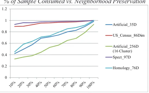
We run 5 comparative tests (usingk=10) with 5 different datasets which are either artificial or taken from the UCI repository [1]. The datasets are:
1. Artificial datasetn=4050,p=35 where the dimensions have distinct characteristics, e.g., normal, log-normal, uniform. 2. US Census Datasetwithn=2216,p=86.
3. An artificial dataset withn=1024,p=256 where the dimensions all together encode 16 clusters. 4. Low Resolution Spectrometerdataset withn=532,p=97.
[image:9.612.174.431.273.433.2]5. Protein Homology Datasetwithn=10498,p=77.
Figure 1 displays theNPRscores for each of the dataset for 10% sample size increments. We observe that with the datasets that are taken from the UCI repository, even with 10% of the data, we obtainedNPRscores close to 1, meaning that there is little difference with the projections computed by using only 10% of the data and those computed by an offline algorithm. However, for artificial datasets with structures, i.e., such as the 16 clusters in Test-3, or with dimensions that have very skewed distributions, i.e., such as log-normal distributions in Test-1, theNPR
scores tend to be lower. This is due to the variability in sampling from these structured dimensions and more advanced sampling schemes may be utilized to overcome these problems [3]. These results show that even with very small portions of the data used, the online algorithm manages to provide approximate results that are reasonably reliable. It has been reported for PCA that in order to obtain reliable results, one has to use
% of Sample Consumed vs. Neighborhood Preservation
0 0.2 0.4 0.6 0.8 1 1.2
Artificial_35D
US_Census_86Dim
Artificial_256D (16 Cluster) Spect_97D
Homology_76D
Fig. 1.Neighborhood preservation ratiovalues computed for 10 different sample sizes for 5 datasets.
at least around 400 items or keep a 10:1 item to dimension ratio, i.e., at least 10 items per dimension [2]. When the amount of data that can be processed by our algorithm in 1 sec. is considered in the above tests (listed in Table 5), we observe that our algorithm manages to process sample sizes that are sufficient to achieve reliable results. The results also show that the number of data items consumed by the algorithm depends on the number of dimensions of the data. As a result, for the 256 dimensional dataset, our sampling method was not able to keep the 10:1 item to dimension ratio in 1 sec. but was able to maintain the 400 items consideration. This implies that for datasets with very large dimension counts, the results of the algorithm may be unstable due to the low number of samples that can be consumed within the temporal limitations.
Moreover, we cross the % of samples in Table 5 with theNPRscores in Figure 1. or three to four iterations (tests 3 and 5).
Test ID # of dimensions # of processed % of data
1 35 1700 41%
2 86 1200 55%
3 256 210 20%
4 97 532 100%
5 77 1330 22%
Table 5. Performance evaluation for online PCA computations (the # and % of items processed in 1 second).
REFERENCES
[1] A. Frank and A. Asuncion. UCI machine learning repository, 2010.
[2] J. Osborne and A. Costello. Sample size and subject to item ratio in principal components analysis. Practical assessment, research & evaluation, 9(11):8, 2004.
[3] M. Pechenizkiy, S. Puuronen, and A. Tsymbal. The impact of sample reduction on pca-based feature extraction for supervised learning. InProceedings of the 2006 ACM symposium on Applied computing, pages 553–558. ACM, 2006.
[4] L. Van der Maaten and G. Hinton. Visualizing non-metric similarities in multiple maps.Machine learning, 87(1):33–55, 2012.