This is a repository copy of
Conceptual design of AM components using layout and
geometry optimization
.
White Rose Research Online URL for this paper:
http://eprints.whiterose.ac.uk/134305/
Version: Accepted Version
Article:
He, L., Gilbert, M. orcid.org/0000-0003-4633-2839, Johnson, T. et al. (1 more author)
(2018) Conceptual design of AM components using layout and geometry optimization.
Computers & Mathematics with Applications. ISSN 0898-1221
https://doi.org/10.1016/j.camwa.2018.07.012
[email protected]
https://eprints.whiterose.ac.uk/
Reuse
This article is distributed under the terms of the Creative Commons Attribution (CC BY) licence. This licence
allows you to distribute, remix, tweak, and build upon the work, even commercially, as long as you credit the
authors for the original work. More information and the full terms of the licence here:
https://creativecommons.org/licenses/
Takedown
If you consider content in White Rose Research Online to be in breach of UK law, please notify us by
Please cite this article in press as: L. He, et al., Conceptual design of AM components using layout and geometry optimization, Computers and Mathematics
Conceptual design of AM components using layout and
geometry optimization
Linwei He
a, Matthew Gilbert
a,*
, Thomas Johnson
b, Tom Pritchard
baFaculty of Engineering, University of Sheffield, UK bLimitState Ltd, Sheffield, UK
a r t i c l e i n f o
Article history: Available online xxxx
Keywords: Layout optimization Geometry optimization Truss
Additive manufacturing
a b s t r a c t
In this paper truss layout optimization is used in conjunction with geometry optimization to provide the basis for a powerful conceptual design tool for additively manufactured (AM) components, particularly useful when the degree of design freedom is high. With layout op-timization the design domain is discretized using a grid of nodes which are interconnected with discrete line elements, forming a ‘ground structure’. Linear optimization can then be used to identify the subset of elements forming the minimum volume structure required to carry the applied loading. A nonlinear geometry optimization step, which involves adjusting the positions of the nodes, can subsequently be undertaken to simplify and improve the solution. Simple geometrical rules can then be used to automatically transform a line element layout into a 3D continuum, ready for validation and/or manufacture. Various extensions to the basic method are described in the paper, including AM build direction constraints and techniques to permit user-interaction with candidate designs, which has been found to be invaluable at the conceptual design stage. Finally the approach described is applied to a range of design problems, including the redesign of an airbrake hinge for the Bloodhound Supersonic Car.
©2018 The Author(s). Published by Elsevier Ltd. This is an open access article under the CC BY license (http://creativecommons.org/licenses/by/4.0/).
1. Introduction
Additive manufacturing (AM, or ‘3D printing’) techniques are developing rapidly, and are now sufficiently mature to be used to produce high value components. However, to benefit from the design freedom AM offers, effective design optimization techniques are required. Although continuum topology optimization techniques such as SIMP [1] have, to date, proved popular for this application, these tend not to perform well if the volume fraction is low (i.e., if the component occupies only a small proportion of the available design space). Also, topology optimization approaches can be computationally expensive and often require labour intensive post-processing in order to realize a practical component. An alternative is to use numerical layout optimization; employing a ground structure [2] to generate least-weight truss designs, which are usually found to be very structurally efficient when the degree of design freedom is high. Using this method, linear programming (LP) can be used to obtain solutions, which ensures the process is robust and computationally efficient, especially when adaptive solution strategies are employed [3,4]. Although the solutions obtained via layout optimization can be complex in form, many such forms can readily be manufactured via AM, leading to renewed interest in the method [5–7]. Furthermore, automatic rationalization techniques (e.g., [8]) can potentially help increase the practicality of a design.
*
Corresponding author.E-mail addresses:[email protected](L. He),[email protected](M. Gilbert),[email protected](T. Johnson),
[email protected](T. Pritchard).
https://doi.org/10.1016/j.camwa.2018.07.012
Please cite this article in press as: L. He, et al., Conceptual design of AM components using layout and geometry optimization, Computers and Mathematics
Although AM can be used to produce components with complex shapes, with many AM processes there are limitations on what can easily be manufactured. For example, in many processes overhanging elements, inclined at shallow angles to the horizontal, can be difficult or impossible to fabricate without support structures. Support structures introduce extra cost and normally require labour to remove them. Addressing this has been the subject of significant attention recently, e.g., [9–13]. Typically continuous topology optimization methods have been used to date, with highly non-linear functions used to impose build direction constraints. This can adversely affect the computational efficiency of the continuum formulation employed (e.g., SIMP), usually already comparatively computationally expensive. On the other hand, when working with a truss idealization the associated optimization problem is much less computationally expensive, and introducing build direction constraints has little or no impact on computational cost. In [14] an optimized truss model is used as a guide that is later mapped onto a continuous model for use by topology optimization methods. However, an inefficient layout optimization formulation is employed, and the mapping process does not appear to take account of the physical sizes of members and joints, limiting the potential benefit of the approach. In the present paper a more computationally efficient truss model idealization is used and the build direction problem is addressed via the use of either (i) a hard constraint approach, whereby shallow inclined members are eliminated from the design problem at the outset, or (ii) a soft constraint approach, whereby a cost penalty is associated with members oriented at angles below a specified minimum.
One issue which arises when using layout and geometry optimization in the process is the need to restrict the optimized form to lie entirely within the problem domain. To achieve this there is a need to take account of the physical sizes of the members and joints, rather than to working with dimensionless line element models. If the physical sizes of members are not considered, any geometrically expanded solid model may cross the domain boundary, potentially leading to an unusable design (which, to the authors’ knowledge, has not been considered in previous works, e.g., [7,14]). There is also a need to ensure that geometry optimization keeps the optimized design entirely within the potentially non-convex 3D domain. Furthermore, stress concentrations can occur at joints, and these should be considered when calculating joint geometry. In this paper the sizes of joints and members are included in both the layout and geometry optimization phases, building on the work of [6] with a view to generating practically useable designs.
Real-world AM design requirements can be quite complex and, although mathematical programming formulations can be adapted to enable a wide range of constraints to be included, the associated optimization problems can become challenging to solve. Furthermore, it will often be difficult to foresee all design requirements in advance. Thus here a non-mathematical user-interaction step is included, giving rise to a ‘human-in-the-loop’ optimization process. This concept can be traced back as far as the early 1970s, in the context of multi-objective optimization problems [15,16], and remains the subject of considerable interest, e.g., [17–19]. However, although it has become mainstream in many industrial sectors, little attention appears to have been given to its use in the field of structural optimization. In this case the concept of an ‘optimum’ is replaced with ‘best compromise’, with the aim of providing a fluid, flexible, and efficient design framework capable of meeting the needs of an AM component designer.
The paper is organized as follows: firstly, the fundamental optimization methods employed, i.e., layout and geometry optimization, are reviewed. Then extensions are described to enable build direction constraints, domain restrictions and interactive design problems to be treated. Practical applications of these extensions are then described, with salient issues discussed and conclusions drawn.
2. Layout and geometry optimization
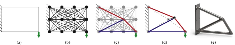
The standard layout optimization process [2–4] involves a series of steps, as shown inFig. 1(a–c). Firstly, the design domain, load and support conditions are specified,Fig. 1(a); secondly, nodes are generated inside the design domain and potential members are created by interconnecting these nodes,Fig. 1(b), forming a ‘ground structure’; finally, the optimal layout is identified by solving the underlying LP problem,Fig. 1(c). The basic single load case rigid-plastic layout optimization formulation can be written as follows:
minV
=
lTa (1a)s.t. Bq
=
f (1b)−
σ
−a≤
q≤
σ
+a (1c)a
≥
0,
(1d)whereVis the volume of the truss structure;l
= [l
1,
l2, . . . ,
lm]
Tis a vector of truss member lengths withmdenoting thenumber of members, anda
= [a
1,
a2, . . . ,
am]
Tis a vector containing the member cross-sectional areas.q= [q
1,
q2, . . . ,
qm]
Tis a vector containing the internal member forces andf
= [f
1x,
f1y,
f1z,
f2x,
f2y,
f2z, . . . ,
fnx,
fny,
fnz]
Tis a vector containing theexternal forces applied on nodes, withndenoting the number of nodes. Also
σ
+andσ
−are limiting tensile and compressive stresses respectively.Bis a 3n×
mequilibrium matrix comprising direction cosines; for memberi, its contribution toBcan be written as:Bi
= [
xIi
−
xIIi li,
y I i−
yII i
li
,
zI i
−
zII i
li
,
xII i
−
xI i
li
,
yII i
−
yI i
li
,
zII i
−
zI i
li
]
TPlease cite this article in press as: L. He, et al., Conceptual design of AM components using layout and geometry optimization, Computers and Mathematics
Fig. 1. Steps in the optimization process: (a) specify design domain, loads and supports; (b) discretize domain using nodes and interconnect these with
potential members, forming a ‘ground structure’; (c) use optimization to identify the subset of members forming the optimal structural layout (blue: compressive; red: tensile); (d) use geometry optimization to improve the solution; (e) convert to a solid geometry model, ready for AM. (For interpretation of the references to colour in this figure legend, the reader is referred to the web version of this article.)
wherexI
i,yIi,zIi,xiII,yIIi andziIIare the nodal positions of the two connected nodes. The optimization variables in(1)are member
areasaand internal forcesq; therefore,(1)is a LP problem, which can be solved efficiently using modern LP solvers such as MOSEK. In addition, by using an adaptive ‘member adding’ scheme (e.g., [3]), medium scale problems (e.g., 1,000,000 design variables) can be solved in a few seconds on a modern desktop PC, with large scale problems (e.g.,
>
1,000,000,000 design variables) also solvable, albeit in a longer time frame.However, in practice, the layout obtained by solving(1)may contain many members having non-zero area, leading to complex truss layouts. This issue was reported in [5,6], where it was also pointed out that the presence of overlapping members and/or nodes in close proximity could be problematic. To address this, geometry optimization [8] can be performed as a post-processing rationalization step (Fig. 1d), which allows the positions of nodes to also be considered as optimization variables. In this case the length termlnow becomes non-linear, resulting in a non-linear programming (NLP) problem. To solve this efficiently, the gradient-based interior point method is adopted, with first and second-order derivatives of all expressions in(1)provided to increase computational efficiency. For example in(1a), assuming the optimization variables for memberiare ordered as
[
xI
i
,
yIi,
ziI,
xIIi,
yIIi,
ziII,
ai,
qi]
, the gradient of member volumeVican be derived as:
▽Vi
=
[
−
Xiaili
−
Yiai li−
Ziai liXiai
li
Yiai
li
Ziai
li
li 0
]
T,
(3)where,Xi
=
xII i−
xI
i,Yi
=
yIIi−
y IiandZi
=
ziII−
z Ii are the projected length of the member of lengthliin the x, y and z axis
directions respectively. Also the Hessian matrix can be derived as:
HVi=
⎡ ⎢ ⎢ ⎢ ⎢ ⎢ ⎢ ⎢ ⎢ ⎢ ⎢ ⎢ ⎢ ⎢ ⎢ ⎢ ⎢ ⎢ ⎢ ⎢ ⎢ ⎢ ⎢ ⎢ ⎢ ⎢ ⎢ ⎢ ⎢ ⎢ ⎣
ai(Y2
i +Z
2
i) l3
i
−aiXiYi l3
i
−aiXiZi l3
i
−ai(Y
2
i +Z
2
i) l3
i
aiXiYi l3
i
aiXiZi l3
i
−Xi li
0
−aiXiYi l3
i
ai(X2
i +Z
2
i) l3
i
−aiYiZi l3
i
aiXiYi l3
i
−ai(X
2
i +Z
2
i) l3
i
aiYiZi l3
i
−Yi li
0
−aiXiZi l3i
−aiYiZi l3i
ai(X2
i +Y
2
i) l3i
aiXiZi l3i
aiYiZi l3i
−ai(X
2
i +Y
2
i) l3i
−Zi li
0
−ai(Y
2
i +Z
2
i) l3i
aiXiYi l3i
aiXiZi l3i
ai(Y2
i +Z
2
i) l3i
−aiXiYi l3i
−aiXiZi l3i
Xi li
0
aiXiYi l3i
−ai(X
2
i +Z
2
i) l3i
aiYiZi l3i
−aiXiYi l3i
ai(X2
i +Z
2
i) l3i
−aiYiZi l3i
Yi li
0
aiXiZi l3i
aiYiZi l3i
−ai(X
2
i +Y
2
i) l3i
−aiXiZi l3i
−aiYiZi l3i
ai(Xi2+Y
2
i) l3i
Zi li
0
−Xi li
−Yi li
−Zi li Xi li Yi li Zi li 0 0
0 0 0 0 0 0 0 0
⎤ ⎥ ⎥ ⎥ ⎥ ⎥ ⎥ ⎥ ⎥ ⎥ ⎥ ⎥ ⎥ ⎥ ⎥ ⎥ ⎥ ⎥ ⎥ ⎥ ⎥ ⎥ ⎥ ⎥ ⎥ ⎥ ⎥ ⎥ ⎥ ⎥ ⎦ .(4)
Please cite this article in press as: L. He, et al., Conceptual design of AM components using layout and geometry optimization, Computers and Mathematics
The resulting structure is normally rational in form, and can then be converted to a solid model by geometrically expanding active nodes/joints to spheres and members to solid cylinders [6], although other, more buckling resistant, cross-sectional types can be used if desired. Finally, a Boolean operation is carried out to generate a unioned solid geometry model suitable for further manipulation, validation via finite element analysis, and/or conversion to a file format readable by an AM machine to enable manufacture,Fig. 1(e).
3. Extensions for the design of AM components
3.1. Build direction in AM
As mentioned earlier, with many AM processes it is not possible to build members inclined at a shallow angle to the horizontal without supports. This gives rise to two challenges: (i) generating an optimized structure that satisfies a specified minimum member inclination requirement; (ii) identifying the build direction which produces the most efficient (e.g., lightest) optimized structure satisfying the latter requirement. To address the first challenge, both a hard constraint approach (which ensures all membersmusthave inclination angles greater than the minimum specified angle) and a soft constraint approach (in which members inclined at shallow angles are penalized, but not prohibited) are now explored.
3.1.1. Hard constraint on member inclination
Using layout optimization, a hard constraint (or limit) on member inclination can be imposed directly since members which do not satisfy this can simply be omitted from the initial ground structure. In the geometry optimization phase, constraints can be added to ensure member directions remain restricted.
Thus, if
θ
mindenotes the minimum member inclination angle, the following constraint can be added for each memberi:sin
θ
min−
⏐
⏐
⏐
⏐
Xidx
li
+
Yidy li+
Zidz li⏐
⏐
⏐
⏐
≤
0,
(5)where,dx,dy,dzare components of a normalized build direction expressed in global Cartesian coordinates.
However, since no members inclined at shallow angles to the horizontal are available for use in the optimization problem, the hard constraint approach may have a severe impact on the structural efficiency of the optimized design. Given that in practice shallow inclined members are usually still manufacturable, albeit at a higher ‘cost’ (due to the need for support structures and post-processing labour work), an alternative soft constraint approach is also investigated.
3.1.2. Soft constraint on member inclination
Using a soft constraint approach, members inclined at an angle to the horizontal below a specified minimum remain present in the problem formulation, but are penalized. This can be achieved by adding a penalty factor that scales up the associated member areas in the objective function(1a):
minV
=
lTPa,
(6)wherePis a diagonal penalty factor matrix with each elementpicalculated using:
pi
=
χ
+
12
+
χ
−
12 tanh(
µ
si−
2),
(7)where
χ
(χ >
1) is a chosen penalty factor for members that do not comply the minimum inclination requirement;µ
is a predefined multiplier (µ
=
20 in this paper), andsiis derived from the inclination constraint(5):si
=
sinθ
min−
⏐
⏐
⏐
⏐
Xidx
li
+
Yidy li+
Zidz li⏐
⏐
⏐
⏐
.
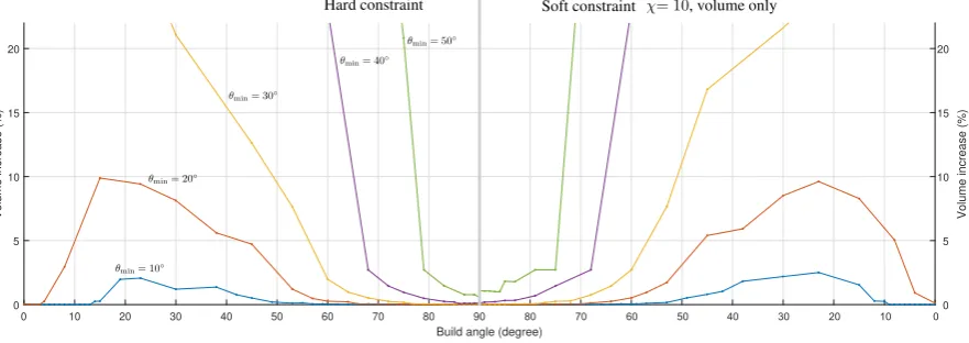
(8)Expression(7) is a smooth Heaviside function used to ensure that members inclined at angles above the specified minimum inclination angle have penalty factors very close to 1.0, whilst members inclined well below this have penalty factors close to the chosen factor
χ
. There exists a transition zone which rapidly increases the penalty from 1.0 toχ
, with the width of this zone primarily governed by the value of multiplierµ
, as shown inFig. 2. Due to the presence of these penalty factors, the optimizer will favour members inclined at angles above the specified minimum inclination angle. In layout optimization, since the angles of members do not change during the optimization process, the linearity of the formulation and associated high computational efficiency are preserved. Note also that after the optimization process has terminated the true volumeVof the structure can readily be computed.3.1.3. Identifying optimal build direction
Please cite this article in press as: L. He, et al., Conceptual design of AM components using layout and geometry optimization, Computers and Mathematics
Fig. 2.Penalty factor applied to members when the specified minimum angle of inclination is 30◦.
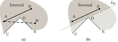
Fig. 3. Restricting member movement in a 2D concave domain: (a) line AB′crosses the design domain boundary after B moves to B′; (b) concave part of
design domain (hatched area) cut off via lineLD.
3.2. Restricting members to lie within a non-convex design domain
In [8] only convex design domains were considered, whereas many real world design examples will involve non-convex design domains. During the geometry optimization stage, nodes and members are required to stay inside the design domain, and this requirement can be achieved by imposing additional constraints on nodal position variables. When convex design domains are involved, it was proposed in [8] that linear constraints be introduced to allow nodes to only move in feasible directions. However, when non-convex design domains are involved, restricting nodes to lie inside the domain is not sufficient, since members can still intersect the boundary (e.g., seeFig. 3(a)). One solution is to convert a concave region into a series of convex ones using domain decomposition, similar to the approach used in [21]. However, for 3D design domains this approach becomes cumbersome. Also, decomposition can significantly reduce the search space, leading to less optimum designs. Here, an alternative approach is adopted: first, the closest point on the boundary to a line segment is identified (e.g., vertex D inFig. 3); second, intersection is prevented by cutting off the concave part via a linear constraint (Fig. 3(b)).
3.3. Restricting finite sized members and joints to lie entirely within a design domain
Traditionally the ground structure based layout optimization method uses a line element representation of members. However, when a generated layout is converted to a solid model, the structure may intersect one or more domain boundaries. Thus if layout optimization is to be used to generate AM components it is essential that the resulting geometry is restricted so as to lie entirely within the design domain. This means that the sizes of members and joints need to be included in the optimization problem formulation. Whilst member sizes can be calculated directly for given cross-section types, calculation of joint size is more complex due to the potential for members to partially overlap in the vicinity of joints, leading to stress concentrations. A pragmatic solution was proposed in [6], which led to satisfactory results being obtained in load test experiments. Here a similar approach is adopted, where for thejth node, the radius of the resulting joint is calculated using:
rj
=
max(rj,i),
i=
1,
2, . . .,
mj,
(9)and,
rj,i
=
√
1 2
π
mj
∑
k=1
[image:6.544.146.399.257.347.2]Please cite this article in press as: L. He, et al., Conceptual design of AM components using layout and geometry optimization, Computers and Mathematics
where,mjis the number of members connected at nodej,
⃗
lj,kandaj,kare the normalized line direction and area of thekthconnected member of nodej, and
⃗
lj,iis the normalized direction of theith connected member. Comparing(10)with theexpression used in [6],(10)does not include non-smooth Macaulay brackets, and leads to more conservative outcomes (i.e., larger joint radii). Also, in [6], joint expansion is a post-processing step, after which joints can potentially intersect a domain boundary, such that a further post-processing iteration is required, whereas the sizes of joints and members are here included directly in the optimization problem formulation.
3.3.1. Layout optimization stage
In the layout optimization stage node positions are fixed. In this case maximum node radii depend on the proximity of a domain boundary. Thus, nodes lying on a boundary must have zero joint radius, which means that they cannot be used in the final design. To address this, the nodal grid can be effectively offset into the design domain so that all nodes initially lie within it. Here, to identify their final position, an iterative approach is used:
1. Solve the layout optimization problem without accounting for the sizes of joints and members.
2. Calculate the joint radius for each node using(9)and(10)and then check if all unsupported and unloaded joints lie entirely within the design domain. If yes, terminate; else proceed to the next step.
3. Find joints that intersect a design domain boundary and offset them into the design domain. If the maximum offset distance for all joints is smaller than a given tolerance, terminate; else proceed to the next step.
4. Update problem matrices using new nodal positions and all active members. Repeat from step 1.
Note that, in cases where the design domain is very restrictive, it may be impossible to fit joints and/or members entirely within it due to their large physical sizes; in such cases, corresponding to cases where the volume fraction is high, a continuum topology optimization approach may be more appropriate.
3.3.2. Geometry optimization stage
In the geometry optimization stage nodes can be moved, such that the allowable joint radius increases when a node is moved away from a boundary and vice versa. The optimizer will seek to find the best outcome and corresponding minimum structural volume. This only requires inclusion of the joint radius variablerjin the design domain constraints. Thus, for
example, a plane constraint becomes:
Txxj
+
Tyyj+
Tzzj+
rj+
Tc≤
0,
(11)whereTx,Ty,TzandTcare coefficients determined by plane normal and the initial position of nodej.
3.4. Interactive design
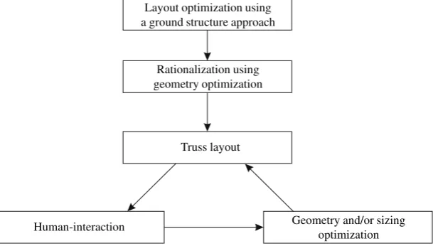
In practice, a design engineer will seldom be able to foresee all possible design considerations in advance of performing an optimization. Also, some design requirements are difficult to define mathematically (e.g., aesthetic considerations). Thus it is useful to include the possibility for human intervention in the design process, allowing a generated design to be modified. A flowchart for the proposed interactive design optimization approach is shown inFig. 4. Firstly an optimum truss design is generated by solving the associated layout and geometry optimization problems, providing a good starting point. The designer can then interact with the model, such as manually editing the layout by adding, moving or deleting structural elements, or specifying new design requirements. Once an intervention has been made, the design can, if desired, then be improved via application of geometry and/or sizing optimization techniques.
However, after a truss has been edited by the user it is likely that equilibrium will have been lost. To address this, and to allow the optimization process to be continued, equilibrium constraints are relaxed and the residuals are penalized, for example, constraint(1b)is relaxed to:
Bq
=
f+
fs,
(12)and the objective function(1a)is changed to:
minV
=
lTa+
µ
s∥
fs∥
1,
(13)where,fsis a ‘virtual’ external force vector, and
µ
sis a penalty factor (here its value is taken as 20V0, whereV0is a reference volume). While equilibrium conditions are now satisfied temporarily, geometry optimization is used to seek to drivefsto zero, whilst also satisfying all existing constraints.Please cite this article in press as: L. He, et al., Conceptual design of AM components using layout and geometry optimization, Computers and Mathematics
Fig. 4.Flowchart for interactive (‘human-in-the-loop’) design optimization approach.
4. Design examples
A range of design examples illustrating the methods described will now be presented, initially using idealized 2D line element models to avoid the results being coloured by extraneous considerations, and then switching to more realistic solid geometry models. In the former case, the methods have been incorporated in a MATLAB script whilst, in the latter case, these have been incorporated in the publicly available LimitState:FORM design optimization software [22]. Note that although many of the examples considered are, for sake of simplicity, 2D forms, which could in many cases be additively manufactured without build direction constraints in practice (if a given truss is constructed with its plane parallel to the build plate, starting directly on the build plate), the methods described are applicable to more complex 3D forms where build direction constraints are potentially useful.
4.1. AM build direction examples
4.1.1. Influence of nodal density
The efficacy of the build direction constraint is affected by the nodal grid employed when using layout optimization. To investigate this the Messerschmidt–Bölkow–Blohm (MBB) beam problem is considered, as shown inFig. 5. This design problem has already been studied by a number of workers in the context of AM build direction constraints (e.g., [9,13,14]). The number of nodal divisions used to discretize lengthLof the design domain is specified, e.g., 4 nodal divisions results in 13
×
5 nodes evenly distributed in a grid, assuming only half the domain is modelled due to symmetry.It is found that when a favourable build direction is employed (e.g., left to right in this case), and a low minimum inclination angle
θ
minis specified, that the use of a coarse nodal grid does not have a significant impact on the results, as shown inFig. 6(a). Also, the impact on the structural volume is less than 3%, compared to the solution obtained without build direction constraints, using 32 nodal divisions. However, after increasing the minimum inclination angleθ
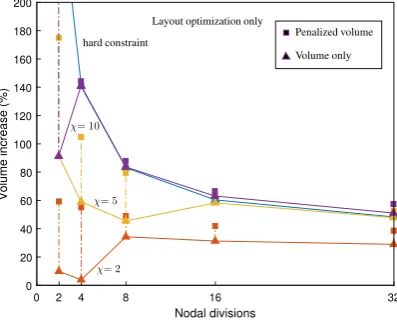
minto 60◦ , the use of a coarse nodal grid leads to significant differences, as shown inFig. 6(b). Solutions generated when using the hard constraint approach exhibit high volume increases, and the optimization even failed to obtain solutions when coarse nodal grids were used, due to the limited number of members in the ground structure. Also, when using the soft constraint approach, although relatively structurally efficient forms were identified, inclination requirements were not fully complied with when low values of the penalty factorχ
were used, seeFig. 7.When the build direction is rotated by 90◦similar behaviour is observed for the 30◦minimum angle of inclination case, as shown inFigs. 8and9. Although the objective function (i.e., the penalized volume) decreases monotonically, the actual volume does not follow the same trend. In other words, less structurally efficient solutions are generated in order to take account of the manufacturing cost constraint. Depending on the value of the penalty factor
χ
, the soft constraint seeks the best compromise between structural efficiency and manufacturing cost. However, in practice the relative importance of structural efficiency and manufacturability will change on a case-by-case basis, something that can be controlled by adjustingχ
(andµ
in(7)).4.1.2. Varying build direction and minimum angle of member inclination
Please cite this article in press as: L. He, et al., Conceptual design of AM components using layout and geometry optimization, Computers and Mathematics
[image:9.544.58.493.218.378.2]Fig. 5.MBB beam example: details of geometry and loading.
Fig. 6.MBB beam example: influence of varying number of nodal divisions, assuming left to right build direction: (a) minimum angle of member inclination
θmin = 30◦; (b) minimum angle of member inclinationθmin = 60◦. (Reference volume calculated using 32 nodal divisions without build direction
considerations.)
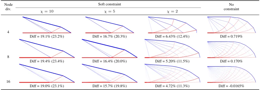
Fig. 7. MBB beam example: rationalized layouts assuming left to right build direction and minimum angle of member inclinationθmin=60◦. (Volume
difference based on layout optimization solution using 32 nodal divisions without build direction considerations; differences in objective function shown in brackets.)
[image:9.544.50.497.428.584.2]Please cite this article in press as: L. He, et al., Conceptual design of AM components using layout and geometry optimization, Computers and Mathematics
Fig. 8.MBB beam example: influence of varying number of nodal divisions, assuming vertical build direction and a minimum angle of member inclination
θmin=30◦. (Reference volume calculated using 32 nodal divisions without build direction considerations.)
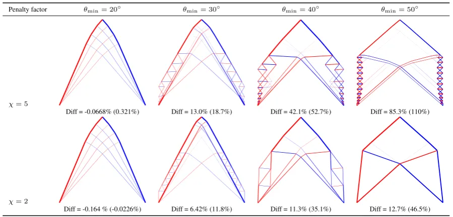
Fig. 9. MBB beam example: rationalized layouts, assuming vertical build direction and minimum angle of member inclinationθmin = 30◦. (Volume
difference based on layout optimization solution using 32 nodal divisions without build direction considerations; differences in objective function shown in brackets.)
On the other hand, when using a less optimum build direction, solutions quickly become very inefficient as
θ
minincreases. Tension and compression bars are replaced by ‘spring-like’ micro structures, reducing structural efficiency, e.g., see the bottom-right layout inFig. 12. In this example, it can be observed that build direction has a much more significant impact on the solution thanθ
min. Therefore in practice it is crucial to identify the best build direction. However, if for some reason the build direction cannot be identified, these inefficient design solutions can be avoided by using smaller penalty factors (Fig. 13), although in this case the minimum inclination requirements are compromised in the interests of improved structural efficiency.4.1.3. Comparison with continuum topology optimization results
To demonstrate the comparative computational efficiency of layout and geometry optimization compared with contin-uum topology optimization methods, a simple 2D Hemp cantilever design example is studied (Fig. 14). Although there is no boundary restriction in this case, a 3L
×
3Lsquare domain (enclosed by dashed lines) is used in the layout optimization, discretized using 16×
16 nodes. A vertical build direction with a minimum angle of member inclinationθ
min=
45◦is considered, in conjunction with a soft constraint approach employingχ
=
10. To facilitate comparison between a truss model and a 2D continuum solid, the physical sizes of the truss members and joints are calculated with their shape ‘flattened’ to a 2D plane (assuming members have rectangular cross-section of unit thickness, and joints are cylindrical with unit thickness). Also note that(10)is replaced with the following expression to take into account the ‘flattened’ shape:rjf,i
=
1 4mj
∑
k=1
[image:10.544.48.494.263.424.2]Please cite this article in press as: L. He, et al., Conceptual design of AM components using layout and geometry optimization, Computers and Mathematics
[image:11.544.55.496.208.364.2]Fig. 10.Vertical cantilever example: details and potential build directions.
Fig. 11.Vertical cantilever example: parametric study by varying build direction and minimum inclination angle.
Fig. 12.Vertical cantilever example: rationalized layouts obtained using soft constraint approach (χ=10) inFig. 11(volume difference based on layout optimization solution using 20 nodal divisions without build direction requirement; differences of objective function in brackets).
[image:11.544.50.495.400.614.2]Please cite this article in press as: L. He, et al., Conceptual design of AM components using layout and geometry optimization, Computers and Mathematics
Fig. 13.Vertical cantilever example: rationalized layouts under soft constraints with lower penalty factor for the problem inFig. 10, using a build direction of 0◦(volume difference based on layout optimization solution using 20 nodal divisions without build direction requirement; differences of objective
function in brackets).
Fig. 14.Hemp cantilever: a comparison of the solutions obtained via layout optimization and continuum topology optimization.
a slight overestimation as it does not account for overlapping regions, e.g., where several members meet a joint.) To account for the build direction in topology optimization, the angle filter proposed in [12] is adopted, which can directly be used in conjunction with the well-known 88-line SIMP script [23]. Two alternative optimization methods are employed, namely the method of moving asymptotes (MMA) (see [24]) and the optimality criteria (OC) method. All quoted CPU costs inFig. 14are obtained using MATLAB on a mobile workstation equipped with Intel i7-7700HQ CPU running 64-bit Windows 10. In the interests of fairness, the CPU results for the SIMP method only include the time taken to solve the linear equations resulting from the finite element analysis, and the time spent by the optimizer (i.e., the MMA or OC routine). The cost of other sections of the code, e.g., filtering or sensitivity analysis, were not taken into account as these could potentially be speeded up, e.g., by using compiled routines. However, for the layout and geometry optimization, the full costs of solving problem(1)with the ‘member adding’ scheme, and that of solving the NLP geometry optimization problem, are included.
[image:12.544.44.498.343.511.2]Please cite this article in press as: L. He, et al., Conceptual design of AM components using layout and geometry optimization, Computers and Mathematics
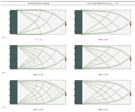
Fig. 15.Horizontal cantilever example: (a) optimized designs neglecting sizes of members and joints; (b) as (a) but with nodal grid offset (by 6 mm) in the vertical direction; (c) optimized designs obtained using the proposed approach.
a maximum of 200 iterations is reached), even though a relaxed stopping criterion is used, with the infinity norm of the changes of variable values between two adjacent iterations increased from 0.01 to 0.05 when using MMA. Also, with the introduction of the non-linear angle filter, the performance of SIMP becomes more sensitive to the choice of parameter values. For example, the variable move limit in OC is reduced from 0.2 to 0.05 to avoid a low quality local optimum solution from being obtained, as reported in [12]. With MMA, the default configuration yields a comparatively inefficient structural form (case III inFig. 14), and a better solution can be generated if variables are only allowed to vary
±
10% of their value in the previous iteration, rather than allowing them to vary across the full range, from 0 to 1.0. In contrast, layout optimization quickly converges to a globally optimal solution for the given nodal discretization, which then provides a good starting point for geometry optimization, thereby increasing the likelihood of converging to an acceptable solution.4.2. Domain limit examples
Considering the previous examples, the physical sizes of the members and joints need to be considered when generating corresponding continuum solid models. Also, if there is a design domain restriction, the techniques introduced in Section3.3
Please cite this article in press as: L. He, et al., Conceptual design of AM components using layout and geometry optimization, Computers and Mathematics
5 12272 0 4545
Firstly, solutions for the case when the physical sizes of members in the solid model are neglected are shown inFig. 15(a). However, since violations of the design domain can be measured, the nodal grid can potentially be offset in the vertical direction to compensate for this (by 6 mm in this case), as shown inFig. 15(b). Since this means that the required physical sizes of the members are likely to change, further violation of the domain will occur, which needs to be addressed; thus a potentially cumbersome iterative solution process is required. Thus the approach proposed in Section3.3is used here to generate the solutions shown inFig. 15(c), i.e., generating viable designs automatically.
Considering the designs obtained inFig. 15(b) and (c), changes to the original nodal grid leads to different layouts being obtained. In particular, more material is required to carry the applied load due to the shorter support length available (4.4% and 4.0% volume increases in (b) and (c), respectively, without the build direction constraint). Thus when moving between line element and solid models, and vice versa, the physical sizes of members should be taken into account, something that appears to have been ignored in most previous studies (e.g., [7,14,25]).
4.3. Conceptual design of a satellite antenna mount
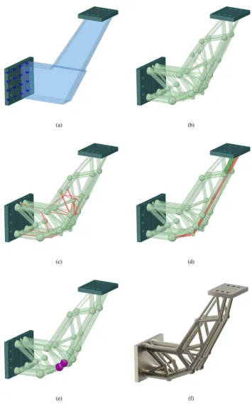
To illustrate the interactive design process, the conceptual design of a satellite antenna mount is considered, as shown in
Fig. 16(a). The component is supported by a vertically aligned rigid plate, with a point load applied to a horizontally aligned rigid plate. The same Ti6Al4 material as used in the previous example is used. Using layout and geometry optimization, an initial design can be generated, as shown inFig. 16(b). To improve the practicality of the design a number of manual interventions can now be made, using the interactive design functionality described in Section3.4. Firstly, all thin members that may be prone to buckling are removed,Fig. 16(c). Secondly, other members deemed undesirable are identified and removed (with replacement members also added as necessary),Fig. 16(d). Thirdly, nodes in close proximity are merged,
Fig. 16(e). During these interventions, equilibrium is relaxed temporarily using constraint(12), and then restored using geometry optimization. The modified component design is then re-optimized to produce a final design,Fig. 16(f).
These steps together increase the structural volume by only 3%, and render the component practical, and potentially ready for additive manufacture. It is also worth noting that this whole process, including the original optimization and all edits, took less than 5 minutes on a standard desktop PC.
4.4. Design of airbrake hinge for the Bloodhound Supersonic Car
The Bloodhound Supersonic Car project aims to build a supersonic car that will reach a speed of 1000 mph (1600 km/h). To achieve this speed it is important that components of the car are as light as possible. There is also a need to slow down the car after the top speed has been reached, which is why airbrakes are needed.
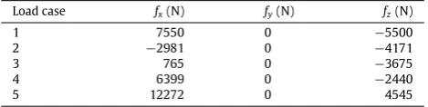
Here the layout and geometry optimization methods described herein will be utilized to investigate the potential weight savings that can be achieved by redesigning the airbrake hinge shown inFig. 17(a), (b), building on the work described in [6]. The design domain shown inFig. 17(c) was derived from the original design and will also be used here. Also, details of the five load cases involved are shown inTable 1(showing load magnitudes prior to applying a safety factor of 2.5).
The truss-like design obtained by Smith et al. [6], shown in Fig. 17(d), was 69% lighter than the original (Table 2), demonstrating the great potential of using layout optimization techniques. The component was manufactured using the Electron Beam Melting (EBM) process, with complementary process modification work undertaken to obviate the need to specify a minimum member inclination angle [26]. However, geometry optimization was not implemented, initially leading to somewhat impractical designs being obtained. This was addressed by manually adjusting the nodal grid and re-optimizing until a suitable design was obtained. The need for human intervention in this case made the full design process tedious and time consuming. It can also be observed that the resulting component, shown inFig. 17(d), is still somewhat complex in form.
[image:14.544.154.389.87.146.2]Please cite this article in press as: L. He, et al., Conceptual design of AM components using layout and geometry optimization, Computers and Mathematics
Please cite this article in press as: L. He, et al., Conceptual design of AM components using layout and geometry optimization, Computers and Mathematics
Fig. 17. Bloodhound airbrake hinge: (a) original component design; (b) original manufactured component, shown in-situ; (c) problem specification for
layout and geometry optimization; (d) physical component designed and manufactured by Smith et al. [6] in Ti6Al4 using the EBM process.
Fig. 18. Bloodhound airbrake hinge: (a) visualization of design obtained using the interactive design approach described in this paper; (b) physical
component manufactured in Ti6Al4 using the SLM process.
5. Discussion
[image:16.544.86.458.429.580.2]Please cite this article in press as: L. He, et al., Conceptual design of AM components using layout and geometry optimization, Computers and Mathematics
Table 2
Bloodhound airbrake hinge: comparison between designs.
Designs Volume (cm3) Diff %
Original continuous design 113a 278.7
Truss-like design (Fig. 17(d), after [6]) 35.27 18.1 New truss-like design (Fig. 18(a)) 35.53 19.0 Extrapolated minimum volume design (after [6]) 29.87 0.0
aInitial volume of 189 cm3scaled down due to difference in material properties;
see [6].
limits dominate, though when multiple load cases are involved there is no guarantee that the layout so obtained will be strictly optimal.
The approach described herein adopts a truss idealization, where the optimized truss layout is transformed into a solid model through simple geometric expansion. However, when this transformation occurs the joints will in reality become rigid, and hence capable of transmitting bending moments (assumed to be absent in the truss idealization). These moments will be relatively small in skeletal structures, but will become increasingly significant as the proportion of the domain occupied by the component increases. If the material used to form the component is ductile then plastic theory indicates that the presence of moments will not adversely affect the load carrying capacity, assuming that elastic deformations prior to failure remain small. Supporting this, in load tests carried out on AM truss specimens by Smith et al. [6] the design load carrying capacity was successfully reached. However, if stress magnitudes are of concern, then cross-sectional areas need to be increased in the geometric expansion stage, over and above the joint size dimensions described by expressions(9)and(10).
In the field of structural optimization the usual goal is to develop optimization tools which are fully automated; thus the proposed interactive ‘human-in-the-loop’ optimization framework represents something of a departure from normal practice. However, the needs of industry are ever changing and thus there is a need for optimization tools that not only tackle engineering design problems efficiently, but which are also highly flexible. When all possible design criteria are considered simultaneously the associated optimization problem generally becomes so computationally challenging that either only very small scale problems can be tackled, or the designer has to make do with solutions which are far from globally optimal. In addition, industrial designs tend to be multi-objective, where compromises need to be made. Instead of utilizing heuristic algorithms, or proposing trade-offs in advance of the optimization, an alternative is to present designs to the user and to let them interactively modify them to achieve the best compromise. Thus the aim of the proposed interactive optimization capability is to provide a quick and effective means of generating designs satisfying industrial needs. In this study, human interaction is limited to relatively minor interventions which do not radically alter the final design. For example, the volumes of most of the designs considered herein are not dramatically changed (e.g., 3% increase in the case of the satellite mount design, shown inFig. 16). Thus here human input is used simply to refine and ‘make practical’ designs generated via mathematical optimization.
6. Conclusions
In the paper, layout optimization is used in tandem with a geometry optimization step to generate structurally efficient design concepts. To enable real-world additive manufacture (AM) component design problems to be tackled, a number of extensions to the basic approach have been made:
•
Firstly, to take account of difficulties associated with manufacturing elements inclined at shallow angles to the horizontal in certain AM processes, two possible approaches are considered (i) a hard constraint approach which directly removes shallow inclined members from the design problem, and (ii) a soft constraint approach which penalizes members below a specified inclination angle. Both are computationally inexpensive, though the soft con-straint approach has the advantage of enabling the designer to balance structural efficiency and manufacturability as desired.•
Secondly, since many real-world design problems involve complex non-convex 3D domains, the geometry optimiza-tion step has been extended to include constraints on the locaoptimiza-tions of joints and members in order to ensure these stay entirely within the design domain. Also, to facilitate this, an effective means of taking account of the physical sizes of joints and members in the optimization problem formulation has been developed.•
Thirdly, an interactive, ‘human-in-the-loop’, optimization framework has been proposed in which human intervention is included as an intrinsic part of the optimization process. This allows the designer to take account of a range of issues not explicitly described in the original optimization problem definition. This involves using geometry optimization to restore equilibrium after a modification has been made by a user.Please cite this article in press as: L. He, et al., Conceptual design of AM components using layout and geometry optimization, Computers and Mathematics
[1] M.P. Bendsøe, O. Sigmund, Topology Optimization: Theory, Methods and Applications, second ed., Springer Science & Business Media, 2003.
[2] W.S. Dorn, R.E. Gomory, H.J. Greenberg, Automatic design of optimal structures, J. Mecanique 3 (1964) 25–52.
[3] M. Gilbert, A. Tyas, Layout optimization of large-scale pin-jointed frames, Eng. Comput. 20 (8) (2003) 1044–1064.
[4] T. Pritchard, M. Gilbert, A. Tyas, Plastic layout optimization of large-scale frameworks subject to multiple load cases, member self-weight and with joint length penalties, in: Proc. of 6th World Congresses of Structural and Multidisciplinary Optimization, Rio de Janeiro, Brazil, 2005.
[5] C.J. Smith, I. Todd, M. Gilbert, Utilizing additive manufacturing techniques to fabricate weight optimized components designed using structural optimization methods, in: Solid Free. Fabr. Symp, 2013, pp. 879–894.
[6] C.J. Smith, M. Gilbert, I. Todd, F. Derguti, Application of layout optimization to the design of additively manufactured metallic components, Struct. Multidiscip. Optim. 54 (5) (2016) 1297–1313.
[7] T. Zegard, G.H. Paulino, Bridging topology optimization and additive manufacturing, Struct. Multidiscip. Optim. 53 (1) (2016) 175–192.
[8] L. He, M. Gilbert, Rationalization of trusses generated via layout optimization, Struct. Multidiscip. Optim. 52 (4) (2015) 677–694.
[9] A.T. Gaynor, J.K. Guest, Topology optimization considering overhang constraints: Eliminating sacrificial support material in additive manufacturing through design, Struct. Multidiscip. Optim. 54 (5) (2016) 1157–1172.
[10] A.M. Mirzendehdel, K. Suresh, Support structure constrained topology optimization for additive manufacturing, Comput. Aided Des. 81 (2016) 1–13.
[11] M. Langelaar, Topology optimization of 3D self-supporting structures for additive manufacturing, Addit. Manuf. 12 (2016) 60–70.
[12] M. Langelaar, An additive manufacturing filter for topology optimization of print-ready designs, Struct. Multidiscip. Optim. 55 (3) (2017) 871–883.
[13] G. Allaire, C. Dapogny, R. Estevez, A. Faure, G. Michailidis, Structural optimization under overhang constraints imposed by additive manufacturing technologies, J. Comput. Phys. 351 (2017) 295–328.
[14] Y. Mass, O. Amir, Topology optimization for additive manufacturing: accounting for overhang limitations using a virtual skeleton, Addit. Manuf. 18 (2017) 58–73.
[15] R. Benayoun, J. de Montgolfier, J. Tergny, O. Laritchev, Linear programming with multiple objective functions: Step method (stem), Math. Program. 1 (1) (1971) 366–375.
[16] J. Wallenius, Comparative evaluation of some interactive approaches to multicriterion optimization, Manage. Sci. 21 (12) (1975) 1387–1396.
[17] D. Meignan, S. Knust, J. Frayret, G. Pesant, N. Gaud, A review and taxonomy of interactive optimization methods in operations research, ACM Trans. Interact. Intell. Syst. 5 (3) (2015) 17:1–17:43.
[18] G.W. Klau, N. Lesh, J. Marks, M. Mitzenmacher, Human-guided search, J. Heuristics 16 (3) (2010) 289–310.
[19] K. Miettinen, F. Ruiz, A.P. Wierzbicki, Introduction to multiobjective optimization: interactive approaches, in: J. Branke, K. Deb, K. Miettinen, R. Słowiński (Eds.), Multiobjective Optimization: Interactive and Evolutionary Approaches, Springer Berlin Heidelberg, Berlin, Heidelberg, 2008, pp. 27–57.
[20] M.J.D. Powell, An efficient method for finding the minimum of a function of several variables without calculating derivatives, Comput. J. 7 (2) (1964) 155–162.
[21] L. He, M. Gilbert, Automatic rationalization of yield-line patterns identified using discontinuity layout optimization, Int. J. Solids Struct. 84 (2016) 27–39.
[22] LimitState Ltd, LimitState:FORM, Version 3.2, Sheffield, UK.<http://limitstate3d.com/limitstateform>.
[23] E. Andreassen, A. Clausen, M. Schevenels, B.S. Lazarov, O. Sigmund, Efficient topology optimization in MATLAB using 88 lines of code, Struct. Multidiscip. Optim. 43 (1) (2011) 1–16.
[24] K. Svanberg, The method of moving asymptotes - a new method for structural optimization, Internat. J. Numer. Methods Engrg. 24 (2) (1987) 359–373.
[25] O. Sigmund, N. Aage, E. Andreassen, On the (non-)optimality of Michell structures, Struct. Multidiscip. Optim. 54 (2) (2016) 361–373.