Kinetic simulations of X-B and O-X-B mode conversion and its deterioration at high input power

deterioration at high input power

.

White Rose Research Online URL for this paper:

http://eprints.whiterose.ac.uk/111957/

Version: Accepted Version

Article:

Arefiev, A. V., Dodin, I. Y., Köhn, A. et al. (4 more authors) (2017) Kinetic simulations of

X-B and O-X-B mode conversion and its deterioration at high input power. Nuclear Fusion.

ISSN 1741-4326

https://doi.org/10.1088/1741-4326/aa7e43

[email protected] https://eprints.whiterose.ac.uk/ Reuse

Items deposited in White Rose Research Online are protected by copyright, with all rights reserved unless indicated otherwise. They may be downloaded and/or printed for private study, or other acts as permitted by national copyright laws. The publisher or other rights holders may allow further reproduction and re-use of the full text version. This is indicated by the licence information on the White Rose Research Online record for the item.

Takedown

If you consider content in White Rose Research Online to be in breach of UK law, please notify us by

Kinetic simulations of X-B and O-X-B mode conversion and its deterioration

at high input power

A. V. Arefiev,1, 2_{I. Y. Dodin,}3_{A. K¨ohn,}4 _{E. J. Du Toit,}5_{E. Holzhauer,}6_{V. F. Shevchenko,}7_{and R. G. L. Vann}5 1)_{Institute for Fusion Studies, The University of Texas, Austin, Texas 78712,}

USA

2)_{Center for High Energy Density Science, The University of Texas, Austin, Texas 78712,} USA

3)_{Princeton Plasma Physics Laboratory, Princeton University, Princeton, New Jersey 08543,} USA

4)_{Max Planck Institute for Plasma Physics, D-85748 Garching, Germany}

5)_{York Plasma Institute, Department of Physics, University of York, York YO10 5DD,} UK

6)_{Institute of Interfacial Process Engineering and Plasma Technology, University of Stuttgart, D-70569 Stuttgart,} Germany

7)_{Tokamak Energy Ltd, 120A Olympic Avenue, Milton Park, Abingdon OX14 4SA,} UK

(Dated: 18 June 2017)

Spherical tokamak plasmas are typically overdense and thus inaccessible to externally-injected microwaves in the electron cyclotron range. The electrostatic electron Bernstein wave (EBW), however, provides a method to access the plasma core for heating and diagnostic purposes. Understanding the details of the coupling process to electromagnetic waves is thus important both for the interpretation of microwave diagnostic data and for assessing the feasibility of EBW heating and current drive. While the coupling is reasonably well– understood in the linear regime, nonlinear physics arising from high input power has not been previously quantified. To tackle this problem, we have performed one- and two-dimensional fully kinetic particle-in-cell simulations of the two possible coupling mechanisms, namely X-B and O-X-B mode conversion. We find that the ion dynamics has a profound effect on the field structure in the nonlinear regime, as high amplitude short-scale oscillations of the longitudinal electric field are excited in the region below the high-density cut-off prior to the arrival of the EBW. We identify this effect as the instability of the X wave with respect to resonant scattering into an EBW and a lower-hybrid wave. We calculate the instability rate analytically and find this basic theory to be in reasonable agreement with our simulation results.

I. INTRODUCTION

A spherical tokamak is one of the concepts consid-ered as a possible future burning plasma device or fu-sion power plant. Results from existing spherical mak experiments increase the understanding of toka-mak physics [1] and extend confinement and threshold databases for next step devices such as ITER. In spher-ical tokamaks the plasma frequency usually exceeds the electron cyclotron frequency (ECF) over the whole con-finement region, characterizing it as overdense. Electro-magnetic waves in the ECF range can therefore not be used directly for heating or current drive. This is a par-ticular disadvantage for spherical tokamaks as they rely on efficient non-inductive current drive mechanisms due to only very little space for a central transformer coil. Electron Bernstein waves (EBWs) [2] are electrostatic waves which can be used instead, since they are very well absorbed at the ECF and its harmonics and provide an efficient method for driving toroidal net currents [3]. Un-derstanding the details of the coupling process between electromagnetic waves and EBWs is important for assess-ing feasibility studies of EBW heatassess-ing and current drive and also for interpreting diagnostics involving EBWs.

At low to intermediate power levels, excitation of EBWs and subsequent current drive has been

demon-strated successfully in spherical tokamaks [4][5]. The linear regime has been extensively studied numerically with ray-tracing [6] and full-wave codes [7] and is well understood. On the other hand, the EBW physics in the nonlinear regime, which is of interest in the context of heating and current drive in modern fusion devices, still presents a challenge [8][9]. Although it has been success-fully demonstrated that the application of high-power EBW heating schemes is in principle possible [10][11], it is of vital importance for upcoming experiments rely-ing on EBWs as a main heatrely-ing or current drive source to understand and quantitatively estimate the losses due to nonlinearities occurring at such high power levels. A complete analytical description of the nonlinear regime is not generally feasible and therefore numerical simula-tions are required.

project involving PIC simulations of upper-hybrid (UH) waves see Ref. [14].) These simulations successfully re-produce X-B and O-X-B mode conversion[6], with both the initial electromagnetic mode and the excited EBW matching the linear dispersion relations. These bench-marking runs confirm that PIC codes are suitable for studies of EBW excitation and, most importantly, they identify the simulation parameters needed to correctly reproduce the mode conversion.

In this work, we use 1D and 2D PIC simulations to examine the mode conversion and associated physics in nonlinear regimes where the wave amplitude is suffi-ciently high to appreciably affect the thermal electron motion. We find that the ion mobility has a profound effect on the wave electric field structure in the non-linear regime. Our kinetic simulations show that high-amplitude short-scale oscillations of the longitudinal elec-tric field are excited in the region below the high-density cut-off prior to the arrival of the EBW generated at the upper-hybrid resonance via a mode conversion. Simula-tions performed with immobile ions show no such short-scale oscillations. Using a detailed analysis of the ion dy-namics in the simulations, we have identified the plasma oscillations driven in the nonlinear regime as lower-hybrid (LH) oscillations. This is in agreement with earlier stud-ies [15][16][17][18] where the X-wave was reported to be-come unstable with respect to backscattering into an EBW and an LH wave. Therefore, our present work can be understood as the first study where this insta-bility is observed in first-principle PIC simulations. We also compare our numerical results with the theory of this scattering instability. The corresponding in-depth theoretical analysis has been published in a companion paper [19].

The rest of the paper is organized as follows. In Sec. II, we describe the setups that we use in our PIC simulations to examine the EBW excitation in the nonlinear regime. Sections III and IV present simulations of the X-B con-version in the nonlinear regime and the corresponding analysis of the ion dynamics. Simulations of the O-X-B conversion in the nonlinear regime are discussed in Sec. V. Section VI provides a theoretical model that we use to explain the origin of the observed instability. Fi-nally, in Sec. VII, we summarize our results and discuss their implication for future experiments with high input power.

II. 1D AND 2D PIC SETUPS FOR STUDYING EBW EXCITATION

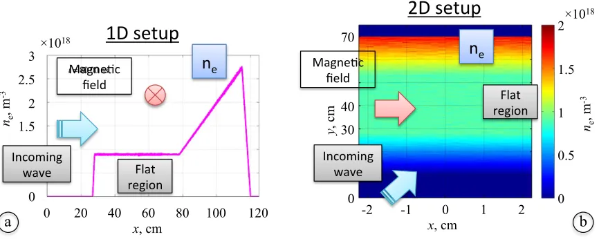
In a recent publication [12], we proposed 1D and 2D setups that are suitable for simulation and clear identifi-cation of the EBW excitation using a standard PIC code (Fig. 1). Both setups have common features that need to be emphasized. A plane incoming wave is injected into a vacuum gap that is deliberately introduced between the plasma and the computational domain boundary on the

injection side. A uniform magnetic fieldB0 that is

par-allel to the injection boundary is initialized throughout the simulation domain. (B0is directed along they-axis in

the 1D setup and along thex-axis in the 2D setup.) The plasma density profile has three distinct regions. Region I, which is on the injection side, corresponds to a steep density profile that includes the UH resonance (UHR). Region II, which is in the middle, corresponds to an ex-tended flat density region. Region III, which is on the opposite side, corresponds to a steep density profile that includes a high-density cut-off for an X-mode.

The multi-gradient density profile makes it convenient to both excite and observe EBWs in the X-B and O-X-B conversions in simulations. Region I is where the EBW excitation takes place. The density gradient in this re-gion needs to be very steep in order to simulate the X-B mode conversion. This scenario relies on X-mode tun-neling past the low-density cut-off and subsequent exci-tation of an EBW in the vicinity of the UH layer. The efficiency strongly depends on the distance between the low-density cut-off and the UH layer and, therefore, it can be dramatically increased by using a steep density gradient. Region II is introduced to aid EBW identifica-tion following its excitaidentifica-tion. There is no density gradient in this extended region, so that the dispersion relation of propagating waves remains unchanged. Finally, Re-gion III is introduced to provide a high-density cut-off for an X-mode. The cut-off reflects an X-mode propa-gating from Region II up the density gradient. We use the steepness of the density profile in this region primar-ily to minimize the size of the simulation domain. There is a vacuum gap between this region and the boundary of the simulation domain in order to eliminate possible numerical boundary artifacts in particle dynamics.

The 2D setup (right panel of Fig. 1) allows for the in-coming waves to be injected at an angle to the applied magnetic field (directed along thex-axis) and to the den-sity gradient (directed along the y-axis). This setup is therefore helpful for achieving and observing an O-X-B mode conversion. Even though a full 2D simulation in which an incoming wave packet has a finite transverse width is possible, it is computationally demanding be-cause the box has to be sufficiently wide to accommo-date the entire path of the wave packet. A “reduced” 2D setup is needed to facilitate multiple runs that are necessary for parameter scans. Such a reduced setup is achieved by using periodic boundary conditions (for par-ticles and fields) on the left and right side of the domain shown in Fig. 1 (right panel). In this setup, the injected wave is a plane wave with given wave-vector components parallel (kk ≡kx) and perpendicular (k⊥ ≡ ky) to the

magnetic field. The transverse size of the domain (along thex-axis) is set to 2π/kk to account for the wave pe-riodicity. We use open boundary conditions at the top and bottom boundaries of the simulation domain. Note that the 1D setup similarly employs open boundary con-ditions.

3

2D setup

Incoming wave

1D setup

Magne5c field

Flat region

Flat region Magne5c

field

Incoming wave

0 20 40 60 80 100 120

x, cm 0

1.5 2 2.5 3 !

1018

ne

, m

-3

-2 -1 0 1 2

x, cm

0 1 2

0.5 1.5

!1018

y

, c

m

0 30 40 70

ne

, m

-3

n

n

a

b

FIG. 1. One and two-dimensional setups for PIC simulations of the X-B and O-X-B mode conversion [12].

20 ns

60 ns

E_z

0 50 100 150 200

x_{, cm} 0

1 2 3 !106

E

,

V

/m

-1

-2

-3

E x E

z

0 50 100 150 200

x_{, cm} 0

1 2 3 !106

E

,

V

/m

-1

-2

-3

0 50 100 150 200

x

, c

m

0 1000 2000 3000

k_{, 1/m}

0 2 4 6 8

am

pl

it

ude

, a

. u.

k-spectrum

0 50 100 150 200

x

, c

m

0 1000 2000 3000

k_{, 1/m}

0 2 4 6 8

am

pl

it

ude

, a

. u.

Immobile ions

k-spectrum

X-mode

EBW EBW

tunneled & reflected

EBW

EBW tunneled

X-mode

tunneled & reflected

E

E

20 ns

60 ns

a b

c d

FIG. 2. 1D PIC simulation of the X-B mode conversion in a nonlinear regime withimmobile ions.

in mind when choosing the density in the flat region in both setups: 1) if O and X modes are not desired in the flat region (Region II), then its density should be above the high-density cutoff; 2) the wavelength of the EBW that decreases with density must be large enough compared to the grid size in order to resolve the EBW oscillations; 3) the amplitude of the numerical field fluc-tuations that increases with density for a fixed number

of macro-particles per cell must be much less than the amplitude of the expected EBW signal.

Using the described 1D and 2D setups, we have per-formed PIC simulations of EBW excitation by waves with a relatively low amplitude (105 _{and 5×10}4 _{V/m). We}

benchmark-ing runs confirm that PIC simulation is suitable for stud-ies of EBW excitation and, most importantly, they iden-tify the simulation parameters needed to correctly repro-duce the mode conversion. In this work, we use the 1D and 2D setups to examine the mode conversion in non-linear regimes, where the wave amplitude is sufficiently high to affect the thermal electron motion.

III. X-B CONVERSION IN A NONLINEAR REGIME

The primary objective of our study is to investigate excitation of EBWs in a nonlinear regime that we access by increasing the amplitude of the incoming wave. In this regime, the wave distorts the thermal motion of electrons. A PIC code simulation is a fully-kinetic simulation that resolves the electron dynamics, which makes it a well-suited approach for this problem. In the present work we use an explicit second-order relativistic particle-in-cell code EPOCH [13].

We first study an X-B mode conversion scenario that can be examined in a 1D simulation. In the simulations presented below, we use a confining magnetic fieldB0=

0.25 T and an incoming wave with frequencyf = 10 GHz. The peak amplitude of the incoming wave that follows a gradual initial ramp-up is set to 8×105 _{V/m. The size}

of the computational domain is 2 m (6×104 _{cells). The}

wave is injected at the left boundary located at x = 0. The incoming wave is an X-mode whose electric field is polarized along thez-axis.

The initial electron density profile is adopted in the form

ne/ncrit=       

     

0, forx < xb1;

128(x−xb1)/l, forxb1≤x < xL;

0.72, forxL≤x≤xR;

4(x−x2)/l, forxR< x < xb2;

0, forx≥xb2,

(1)

where ncrit≈1.24×1018 m−3 is the critical density for

the chosen frequency. We have introduced the follow-ing quantities to parameterize the multi-gradient density profile: xL = 0.28 m, xR = 1.58 m, ∆x= 0.005625 m,

xb1=xL−∆x,xb2= 1.95 m,x2= 1.4 m, andl= 1 m.

The electron population is initialized using 400 macro-particles per cell. The initial electron temperature is set at Te= 950 eV. We also initialize deuterium ions using

400 macro-particles per cell with the ion number density equal toneand the ion temperature equal toTe.

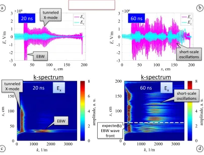
Our first simulation in the nonlinear regime was per-formed with immobile ions. This was motivated by the fact that the ion mobility has no significant impact on the dispersion relation of EBWs in a linear regime. Snap-shots of transverse (Ez) and longitudinal (Ex) electric

field components are shown in the upper panels of Fig. 2 at 20 ns and 60 ns into the simulation. As the X-mode tunnels into the flat density region, it excites an EBW at the sharp density gradient (upper-left panel of

Fig. 2). The corresponding k-spectrum for the longitu-dinal component of the electric fieldEx as a function of

the distance into the plasma is shown in the lower-left panel of Fig. 2. The excited EBW follows the dispersion relation predicted for the linear regime (marked with a dashed vertical line). The right two panels in Fig. 2 show the field profile and the k-space 40 ns later. By this time, the tunneled X-mode has already reflected off the high-density cut-off on the right of the simulation domain and it is moving towards the UH layer. The basic fea-tures of the EBW spectrum however remain unaffected by this large-amplitude reflected wave, similarly to what one would expect in the linear regime.

The second simulation in the nonlinear regime was performed with mobile ions and the results are shown in Fig. 3. The initial stage prior to the X-mode being reflected off the high-density cut-off (left two panels in Fig. 3) is similar to what we observed in the simulation with immobile ions (left two panels in Fig. 2). How-ever, the field structure dramatically changes 40 ns later, as the reflected X-mode starts to propagate through the plasma. As evident from the two right panels in Fig. 3, short-scale oscillations appear throughout the plasma.

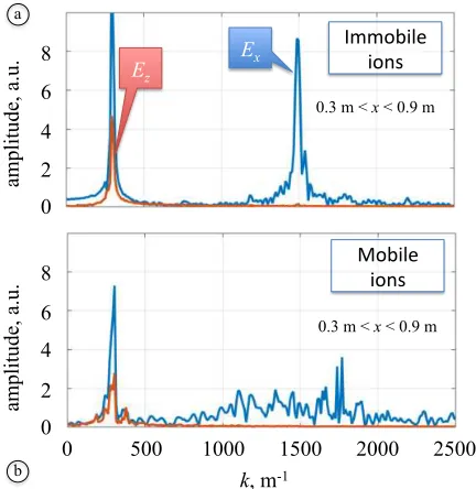
In order to closely examine the differences in the elec-tric field structure for the cases of mobile and immobile ions, we have performed a Fourier analysis of the field in the flat density region at 45 ns into the simulation. It is worth noting that an EBW that is excited in a lin-ear regime at the sharp density gradient would cover less than half of the flat region by this time. We therefore separately consider the left (0.3 m< x <0.9 m) and the right (0.9 m< x <1.5 m) side of the flat density region, with the corresponding spectra shown in Figs. 4 and 5. In the case of immobile ions, short-scale oscillations of the longitudinal electric field are concentrated on the left side of the flat region (compare the two upper panels of Figs. 4 and 5). Their spectrum has a very pronounced peak centered aroundk ≈1500 m−1_{. This is the EBW}

mode that is excited at the sharp density gradient and which propagates from left to right.

In the case of mobile ions, the short-scale part of the Ex spectrum (see lower panels of Figs. 4 and 5) has a

qualitatively different structure from that in the case of immobile ions. The two striking differences are: (i) the absence of a sharp peak centered atk ≈1500 m−1

5

20 ns

60 ns

E_z

0 50 100 150 200

x_{, cm}

0 1 2 3 !106

E

,

V

/m

-1

-2

-3

E_x E

z

0 50 100 150 200

x_{, cm}

0 1 2 3 !106

E

,

V

/m

-1

-2

-3

0 50 100 150 200

x

, c

m

0 1000 2000 3000

k_{, 1/m}

0 2 4 6 8

am

pl

it

ude

, a

. u.

k-spectrum

0 50 100 150 200

x

, c

m

0 1000 2000 3000

k_{, 1/m}

0 2 4 6 8

am

pl

it

ude

, a

. u.

Mobile ions

k-spectrum

X-mode

EBW

short-scale oscilla<ons

EBW

expected EBW wave

front tunneled

X-mode

20 ns

E

60 ns

E

short-scale oscilla<ons

a b

c d

FIG. 3. 1D PIC simulation of the X-B mode conversion in a nonlinear regime withmobile ions.

IV. ION DYNAMICS IN THE NONLINEAR REGIME

In the previous section, we showed that the ion mobil-ity has a profound impact on the electric field structure in the nonlinear regime. In what follows, we explore in detail the ion dynamics in the nonlinear regime in order to gain a better insight into the observed phenomenon.

We have performed an additional simulation in the nonlinear regime with mobile ions, but in this case we ini-tialized the ions as cold. A comparison of the wave struc-ture between this simulation and the simulation with hot ions shows that the wave structure reported in Sec. III remains for the most part unaffected by the ion thermal motion or the lack thereof. We can then conclude that the observed change in the wave structure in the nonlin-ear regime is primarily related to the ion mobility rather than the ion temperature.

In order to examine the ion dynamics in the nonlin-ear regime, we take a closer look at the evolution of the ion momentum. If the ions are initially hot, then their thermal motion makes it technically challenging to de-couple and visualize collective modes in the momentum space. However, since the thermal motion is not a key factor, we can examine the ion dynamics for the case of initially cold ions instead. In this case, the longitudinal ion momentumpx effectively becomes just a function of

x and t, since ions at the same location have a similar

momentum.

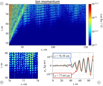
The corresponding plot of the ion momentum ampli-tude in the flat density regions is shown in the upper panel Fig. 6. Not surprisingly, there is a region with strong oscillations that expands from the left side of the domain. This region is associated with an EBW that is excited at the sharp density gradient that is located just to the left of the plotted region. What is surprising is that, in addition to these oscillations, there are also pronounced ion oscillations that seem to originate within the flat density region. The lower-left panel provides a zoomed-in version of the original ion momentum plot. It is evident from this plot that the ions perform periodic longitudinal oscillations whose amplitude grows in time. The lower-right panel gives a time evolution ofpxat two

fixed locations that are marked in the lower-left panel with the dotted lines. It is important to point out that the characteristic time scale of these oscillations is much larger than the period of the incoming wave.

The lower panel of Fig. 7 shows the corresponding k -spectrum of the ion momentum oscillations in the flat density region. In order to isolate the oscillations that originate in the flat density region, the Fourier analysis was performed att= 59 ns for 0.9 m< x <1.2 m and 1.2 m< x <1.5 m. It is instructive to compare the obtained spectrum that has two short-scale modes (k≈1500 m−1

m−1 _{and k ≈ 600 m}−1_{) with the spectra of the}

elec-tric field shown in Figs. 4 and 5 for the cases of mobile and immobile ions. The two pronounced short-scale ion oscillations (k≈1500 m−1_{andk≈2000 m}−1_{) differ}

sig-nificantly from the short-scale longitudinal electric field oscillations shown in the lower panel of Fig. 5. On the other hand, one of the short-scale (k ≈ 1500 m−1_{) and}

one of the long-scale (k ≈ 300 m−1_{) modes appear to}

match the k-vectors of the modes that we observed in the simulation with immobile ions.

The main reason for the apparent disagreement be-tween the ion spectrum (lower panel of Fig. 7) and the electric field spectra in Figs. 4 and 5 is that the ion oscilla-tions are low-frequency oscillaoscilla-tions, whereas the electric field spectra do not distinguish between low-frequency oscillations and the oscillations at the frequency of the incoming wave. In order to examine low-frequency elec-tric field oscillations, we have performed an additional simulation in which time-averaged electric fields were sep-arately calculated by continuously averaging both com-ponents of the field over two cycles of the incoming wave (f = 10 GHz). The result is shown in the upper panel of Fig. 7. The time instant is the same as that for the plot of the ion oscillations in the lower panel of the same figure. The peaks corresponding to the oscillations of the “slow” electric field match those in the ion spectrum, which enabled us to identify the corresponding modes.

It must be pointed out that the units used to normal-ize the vertical scale in Figs. 4 and 5 and in the upper panel of Fig. 7 are the same. The height of the peaks in the slow electric field spectrum is almost an order of magnitude smaller than the height of the peaks in Figs. 4 and 5. It is therefore not surprising that the slow electric

0 2

k_{, m}-1

0 4 6 8

am

pl

it

ude

,

a.u

.

0.3 m < x < 0.9 m

500 1000 1500 2000 2500

E_x E_z

am

pl

it

ude

,

a.u

.

0 2 4 6 8

Immobile

ions

Mobile

ions

0.3 m < x < 0.9 m a

b

FIG. 4. Spectra of the transverse and longitudinal electric field components at 45 ns into the simulation in the flat region for 0.3 m< x <0.9 m.

field oscillations are not easily visible without the time-averaging. The bottom line is that the ion dynamics in the flat density region that arises without the converted EBW is coupled to four “slow” modes: two short-scale modes and two long-scale modes.

V. O-X-B CONVERSION IN A NONLINEAR REGIME

In order to determine whether the excitation of the short-scale electric fields is a robust feature, we have also carried out a 2D PIC simulation. We access the nonlinear regime by setting the amplitude of the incoming wave, injected at an angleθ = 40◦ _{to the density gradient, at} 8×105_{V/m. The wave frequency isf = 10 GHz and its}

electric field is polarized in the plane of the simulation, i.e. it has bothxandy-components. We use a confining magnetic field,B0 = 0.25 T, directed along the x-axis.

The size of the computational domain is 1 m (1.4×104

cells) along they-axis and c/fsinθ (25 cells) along the x-axis. Note that the injection angle of θ = 40◦ _{is the} optimal injection angle [6],

θ_opt≡arcsin

"s

fce

f +fce #

, (2)

that maximizes the power transmission from the O-mode into the slow X-mode for our values of the electron cy-clotron frequency,fce= 7 GHz, and the wave frequency,

f = 10 GHz.

0 0.5

k_{, m}-1

1 1.5

am

pl

it

ude

,

a.u

.

0.9 m < x < 1.5 m

1000 1500 2000 2500

E_x

am

pl

it

ude

,

a.u

.

0 0.5 1 1.5

Immobile

ions

Mobile

ions 0.9 m < x < 1.5 m

E_x

2

2

a

b

7

30

60

90

76

77

78

x

, cm

0

40

80

t

, ns

60

20

t

, ns

p

, kg

m

/s

0

10

-10

x

= 76.38 cm

x

= 77.64 cm

10

30

50

t

, ns

70

90

10

10

10

10

|

p

|, kg

m

/s

Ion momentum

50

100

150

x

, cm

a

b c

FIG. 6. Ion momentum in a 1D PIC simulation of the nonlinear regime with initially cold ions. The lower-left panel is a zoom-in of the upper panel for 76 cm< x <78 cm and 30 ns< t <90 ns. The lower-right panel gives a time evolution of the ion momentum at two fixed locations,x= 76.38 cm andx= 77.64 cm, marked in the lower-left panel with the dotted lines.

The initial electron density profile is given by

ne/ncrit=       

     

0, fory < yb1;

4(y−yb1)/l, foryb1≤y < yL;

0.72, foryL≤y≤yR;

4(y−y2)/l, foryR< y < yb2;

0, fory≥yb2,

(3)

where ncrit≈1.24×1018 m−3 is the critical density for

the chosen frequency. We have introduced the follow-ing quantities to parameterize the multi-gradient den-sity profile: yL = 0.28 m, yR = 0.78 m, yb1 = 0.1 m,

yb2 = 0.95 m, y1 = 0.1 m, y2 = 0.6 m, and l = 1 m.

The electron population is initialized using 400 macro-particles per cell. The initial electron temperature is set at Te = 950 eV. We also initialize cold deuterium ions

using 400 macro-particles per cell with the ion number density equal tone.

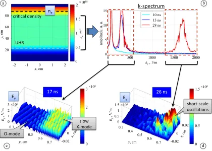
Figure 8 shows snapshots of theEy component of the

electric field (the component directed along the density gradient). The 15 ns snapshot captures the initial stage of an O-mode conversion into a slow X-mode. At 28

ns, the slow X-mode has almost reached the UHR layer where the conversion into an EBW takes place in the linear regime. However, short-scale oscillations have al-ready been excited at this stage on the opposite side of the flat density region (x > 60 cm). This behavior is similar to what is observed in the 1D simulation in the nonlinear regime (see Fig. 3).

In order to better examine the evolution of the field structure, we have computed thek-spectrum of the lon-gitudinal electric field in the flat density region at 10 ns, 13 ns, and 28 ns (see the upper-right panel of Fig. 9). At 10 ns, there is only an O-mode in the flat density region. At 13 ns, a part of the O-mode has already been con-verted into a slow X-mode that shows up as a peak at aroundk⊥ ≈300 1/m. At 28 ns, short-scale oscillations also appear in the spectrum of the longitudinal field.

0 1

k_{, m}-1

0 2 3 4

am

pl

it

ude

,

a.u

.

0.9m < x < 1.2m 1.2m < x < 1.5m

500 1000 1500 2000 2500

E_x E_z

am

pl

it

ude

,

a.u

.

0 0.1 0.2

Ion momentum Slow electric

field

a

b

FIG. 7. Spectra of a slow electric field (a) and of the longi-tudinal ion momentum (b) at 59 ns into the simulation with initially cold ions. The spectra are calculated in the flat re-gion for 0.9 m< x <1.5 m. The slow electric field is a time-average of the electric field over two periods of the incoming wave (f= 10 GHz).

flat density region. Moreover, the short-scale oscillations grow on a timescale shorter than the time required for the O-X-B conversion to take place. They appear in the spectrum before the slow X-mode even reaches the con-version layer located at the UHR. This result is consistent with the excitation of short-scale oscillations in the one-dimensional simulation with mobile ions, which confirms the robustness of the observed phenomenon.

We have performed an additional 2D PIC simulation for the same setup, but this time initializing hot ions (Ti= 950 eV). The short-scale oscillations are again

ex-cited in the flat density region before the slow X-mode even reaches the conversion layer located at the UHR. Additional runs with heavier cold ions show that the amplitude of the short-scale oscillations reduces as we increase the ion mass. This is consistent with our conclu-sion that it is the ion mobility that enables the excitation of the short-scale oscillations in the plasma.

VI. THEORETICAL INTERPRETATION

We interpret the appearance of the small-scale oscil-lations that were described above as an observation of the X-wave instability with respect to scattering into an EBW and a lower-hybrid wave (LHW). This instability was previously discussed in a number of papers; for exam-ple, see Refs. [15][16[17][18]. However, to our knowledge,

we are first to report an observation of this instability in PIC simulations and explore it in detail.

In order to interpret the structure of the observed spa-tial spectra in the context of this instability in simplest terms, we focus on the explanation of the 2D simula-tions. The scattering can be understood as a three-wave interaction satisfying two scalar resonance conditions:

ω(x)_≈ω(ebw)_+ω(lh)_{, k}(x)

x ≈k(ebw)x +k(lh)x . (4)

Hereω(q) _{are frequencies andk}(q)

x are projections of the

corresponding wave vectors on the axis of propagationx. One can expect ω(lh)_≈ω

LH≪ω(x)∼ω(ebw)∼ωUH,

whereωLHandωUHare the lower- and upper-hybrid

fre-quency, respectively. Thus EBWs must be excited at the frequencyω(ebw) _≈ω(x)_−ω(lh)_{. The corresponding}

wave numbers found from the linear dispersion relation arek(ebw)x ≈ ±1750 m−1. Note that the part of the EBW

that is produced through linear _{conversion (without an} LHW being involved) has frequencyω(ebw)_=ω(x)_{, so its}

kx(ebw)must be slightly lower, namely,k(ebw)≈1600 m−3:

this difference can indeed be seen in Fig. 3(d).

As determined by the cold linear dispersion relation, the incident and reflected X waves have wave numbers kx(x)≈ ±300 m−1, in agreement with simulations. Hence,

Eq. (4) predicts two possible values for k(lh)x , namely,

±1450 m−1 _{and ±2050 m}−1_{. This is in agreement with}

Fig. 7, which shows pronounced peaks in the electric field and ion momentum spectra at these expected locations. (Positive and negativekare not distinguished in our fig-ures.) We also point out that, under the specified pa-rameters, 2π/ωLH ≈ 7.9 ns. The temporal oscillations

in Fig. 6(c) have approximately this period, so they can indeed be safely identified as LH oscillations. The peak at|k| ∼600 m−1_{is due to the beating of the LHWs plus}

the contribution of the X-wave’s second harmonic. The peak at |k| ∼300 m−1 _{corresponds to the incident and}

reflected X waves. (Ion velocities _{cannot be perturbed} by the X waves because such waves have frequencies that are too high; however, ionmomenta _{can be.) The} rea-son why the X-wave fields show up on a figure for time-averaged quantities is that the averaging is performed over the period of the unperturbed incident wave. The actual X waves have non-stationary envelopes evolving at rates∼ωLH, so averaging of these fields does not

elimi-nate them entirely.

A detailed analytical study of the instability discussed here is somewhat lengthy, so we report it in a separate paper [19]. Here we present the final answer only. In the regime of interest, the instability rate is expected to be

γ≈ωLH

ωpeωpi

|ΩeΩi| r_ω

LH

ωUH k(lh)E

(x) x

16πene

. (5)

Here, ωpe and ωpi are the electron and ion plasma

fre-quencies respectively, Ωe and Ωi are the electron and

ion cyclotron frequencies,e is the electron charge, ne is

the unperturbed electron density, andEx(x)is thex

9

-2 -1 0 1 2

x, cm

-2 -1 0 1 2

x, cm

y

, c

m

20 40 80

60

y

, c

m

20 40 80

60

-1 !106

Ey

,

V

/m

0 1

0.5

-0.5 15 ns

O-mode slow

X-mode

short-scale oscilla5ons

28 ns

fast X-mode

slow X-mode

E

E

a b

FIG. 8. Snapshots of the electric field transverse to the confining magnetic field from a 2D PIC simulation of the O-X-B mode conversion in the nonlinear regime withmobileions.

17 ns

k-spectrum

0.3 0.4

0.5 0.6

0.7

y, cm -0.02

0.02

0

0 1 2 3 !10

6

0 1 2 3 !106

26 ns

0.3 0.4

0.5 0.6

0.7

y, cm -0.02

0.02

0

0 0.5 1 1.5 !10

6

0 0.5 1 1.5 !106

Ey

,

V

/m

Ey

,

V

/m

-2 -1 0 1 2

x, cm

y

, c

m

20 40 80

60

0 1 2

0.5 1.5

!1018

ne

, m

-3

10 ns 13 ns 28 ns

0 500 1000 1500 2000

ky, 1/m 0

15

10

5

am

pl

it

ude

, a

. u.

UHR

cri5cal density

O-mode

slow X-mode

short-scale oscilla5ons

n_e

E_{y E}

y

a b

c d

FIG. 9. 2D PIC simulation of the O-X-B mode conversion in the nonlinear regime withmobile ions: upper left – simulation setup; upper right –k-spectrum of the longitudinal electric field Ey at 10 ns, 13, and 28 ns into the simulation in the flat density region. The two lower panels show the long-scale (c) and the short-scale (d) contributions toEyat 17 ns and at 26 ns. The corresponding ranges ofky are marked with dashed boxes in the upper-right panel and connected to the corresponding lower panels with arrows.

have no dependence onT, while the dependence on the ion mass remains. This is precisely what is observed in our simulations. More specifically, for our parameters, Eq. (5) gives γ−1 _{≈7.6 ns. This is in reasonable}

agree-ment with Fig. 6(c), especially considering that the figure illustrates the already nonlinear regime and that Eq. (5)

VII. SUMMARY

We have simulated X-B and O-X-B mode conversion in a nonlinear regime where the driving wave apprecia-bly distorts electron thermal motion. We find that the ion mobility has a profound effect on the field structure in this regime. High amplitude short-scale oscillations of the longitudinal electric field are observed in the re-gion below the high-density cut-off prior to the arrival of the EBW. We have additionally performed an exten-sive parameter scan by varying the spatial resolution, the ion mass, and the ion temperature. This scan shows the robustness of the observed effect.

We identify this effect as the instability of the X wave with respect to resonant scattering into an EBW and a lower-hybrid wave. We calculate the instability rate analytically and find this basic theory to be in reasonable agreement with our simulation results.

More generally, the methodology introduced in this pa-per provides the framework for an accurate quantitative assessment of the feasibility of heating and current-drive in next-generation spherical tokamaks by megawatt-level beams.

VIII. ACKNOWLEDGMENTS

This work was funded in part by the US Department of Energy under grants FG02-04ER54742 and DE-AC02-09CH11466, the University of York, the UK EP-SRC under grant EP/G003955, and the European Com-munities under the contract of Association between EU-RATOM and CCFE. Simulations were performed us-ing the EPOCH code (developed under UK EPSRC grants EP/G054940, EP/G055165 and EP/G056803) us-ing HPC resources provided by the Texas Advanced Computing Center at The University of Texas and using the HELIOS supercomputer system at Computational Simulation Centre of International Fusion Energy Re-search Centre (IFERC-CSC), Aomori, Japan, under the Broader Approach collaboration between Euratom and Japan, implemented by Fusion for Energy and JAEA.

1_{A. Sykes, “Overview of recent spherical tokamak results”, Plasma} Phys. Control. Fusion43_{, A127 (2001).}

2_{H. P. Laqua, Plasma Phys. Control. Fusion}49_{, R1 (2007).}

3_{J. Urban, J. Decker, Y. Peysson, J. Preinhaelter, V. Shevchenko,}

G. Taylor, L. Vahala, and G. Vahala, Nucl. Fusion51_{, 083050}

(2011).

4_{S. Shiraiwa, K. Hanada, M. Hasegawa, H. Idei, H. Kasahara, O.}

Mitarai, K. Nakamura, N. Nishino, H. Nozato, M. Sakamoto, K. Sasaki, K. Sato, Y. Takase, T. Yamada, H. Zushi, and Group,

Phys. Rev. Lett.96_{, 185003 (2006).}

5_{V. F. Shevchenko, Y. F. Baranov, T. Bigelow, J. B. Caughman,}

S. Diem, C. Dukes, P. Finburg, J. Hawes, C. Gurl, J. Griffiths, J. Mailloux, M. Peng, A. N. Saveliev, Y. Takase, H. Tanaka, and

G. Taylor, EPJ Web of Conferences87_{, 02007 (2015).}

6_{F. R. Hansen, J. P. Lynov, and P. Michelsen, “The O-X-B mode}

conversion scheme for ECRH of a high-density Tokamak plasma”, Plasma Phys. Controlled Fusion27_{, 1077 (1985).}

7_{A. K¨ohn, J. Jacquot, M. W. Bongard, S. Gallian, E. T. Hinson,}

and F. A. Volpe, Phys. Plasmas21_{, 092516 (2014).}

8_{N. Xiang and J. R. Cary, Phys. Plasmas}18_{, 122107 (2011).}

9_{M. A. Asgarian, A. Parvazian, M. Abbasi, and J. P. Verboncoeur,}

Phys. Plasmas21_{, 092516 (2014).}

10_{H. P. Laqua, V. Erckmann, H. J. Hartfuß, H. Laqua, W7-AS}

Team, and ECRH Group, “Resonant and Nonresonant Electron Cyclotron Heating at Densities above the Plasma Cutoff by O-X-B Mode Conversion at the W7-As Stellarator”, Phys. Rev. Lett.

78_{, 3467 (1997).}

11_{A. Pochelon, A. Mueck, L. Curchod, Y. Camenen, S. Coda, B.}

P. Duval, T. P. Goodman, I. Klimanov, H. P. Laqua, Y. Martin, J.-M. Moret, L. Porte, A. Sushkov, V. S. Udintsev, F. Volpe, and the TCV Team, “Electron Bernstein wave heating of over-dense H-mode plasmas in the TCV tokamak via O-X-B double mode

conversion”, Nucl. Fus.47_{, 1552 (2007).}

12_{A. V. Arefiev, E. J. Du Toit, A. K¨ohn, E. Holzhauer, V. F.}

Shevchenko, and R. G. L. Vann, “Kinetic simulations of X-B

and O-X-B mode conversion”, AIP Conf. Proc. 1689_{, 090003}

(2015) [http://dx.doi.org/10.1063/1.4936540].

13_{T. D. Arber, K. Bennett, C. S. Brady, A. Lawrence-Douglas, M.}

G. Ramsay, N. J. Sircombe, P. Gillies, R. G. Evans, H. Schmitz, A. R. Bell, and C. P. Ridgers, Plasma Phys. Controlled Fusion

57_{, 113001 (2015).}

14_{J. Xiao, J. Liu, H. Qin, Z. Yu, and N. Xiang, Phys. Plasmas}22_,

092305 (2015).

15_{E. Z. Gusakov and A. V. Surkov, “Induced backscattering in an}

inhomogeneous plasma at the upper hybrid resonance”, Plasma

Phys. Control. Fusion49_{, 631 (2007).}

16_{F. S. McDermott, G. Bekefi, K. E. Hackett, J. S. Levine, and}

M. Porkolab, “Observation of the parametric decay instability during electron cyclotron resonance heating on the Versator II

tokamak”, Phys. Fluids25_{, 1488 (1982).}

17_{M. Porkolab, “Parametric decay instabilities in ECR heated}

plas-mas”, in Proceedings of the Second Workshop of the Hot Electron Ring Physics, San Diego, California, December, 1981, edited by N. A. Uckan, National Technical Information Service, U.S. Dept. of Commerce, Report No. CONF-811203, 237 (1982).

18_{A. T. Lin and C.-C. Lin, “Nonlinear penetration of upper-hybrid}

waves induced by parametric instabilities of a plasma in an

in-homogeneous magnetic field”, Phys. Rev. Lett.47_{, 98 (1981).}

19_{I. Y. Dodin and A. V. Arefiev, “Parametric decay instability of}

plasma waves near the upper-hybrid resonance”, Phys. Plasmas