Parabolic equations with continuous initial data

with

Continuous Initial Data

Julie Clutterbuck

April 2004

A THESIS SUBMITTED FOR THE DEGREE OF

The work in this thesis is my own except where otherwise stated.

My fellow students have been an unfailing source of good conversation and interest­ ing mathematics: thankyou Nick Dungey, Andreas Axelsson, Denis Labutin, Jason Sharpies and others at the Australian National University.

My supervisor Ben Andrews has been surprisingly patient over the years, and an excellent and insightful guide.

At the Mathematical Sciences Institute, the administrative and academic staff have been friendly and helpful. Alan McIntosh has been generous with his good advice (which I ignored) and his friendship (which I appreciate).

I thank my dear friend Maria Athanassenas for her support as my mentor.

My family have been wonderful: thankyou to my lovely parents, Sue and Neil, my grandmother Marjorie Anderson, and the rest of them. My friends have remained my friends which is more than I could ask for: thankyou Annabel Barbara, Nathalie Jitnah, Rohan Baxter, Joseph Baxter, Dan Rosauer, Allison Foster, and Nick Lake.

And above all, thanks to my beloved Brendan.

The aim of this thesis is to derive new gradient estimates for parabolic equations. The gradient estimates found are independent of the regularity of the initial data. This allows us to prove the existence of solutions to problems that have non-smooth, con­ tinuous initial data. We include existence proofs for problems with both Neumann and Dirichlet boundary data.

The class of equations studied is modelled on mean curvature flow for graphs. It includes anisotropic mean curvature flow, and other operators that have no uniform non-degeneracy bound.

We arrive at similar estimates by three different paths: a ’double coordinate’ ap­ proach, an approach examining the intersections of a solution and a given barrier, and a classical geometrical approach.

Contents 9

1 Preface 11

2 Mean curvature flow and parabolic equations 15

2.1 Parabolic equations ... 15

2.2 Mean curvature f l o w ... 17

3 Gradient estimates for parabolic equations of curve shortening flow type in one space dimension 21 3.1 Outline of th e ‘double coordinate’ m e th o d ... 22

3.2 An estimate for periodic solutions... 23

3.3 Description of a b arrier... 25

3.4 An explicit estimate for periodic e q u a tio n s... 26

3.5 Interior estimates for non-periodic equations with 6 = 0 ... 30

3.6 A generalisation to fully nonlinear equations... 33

4 An existence result for a parabolic equation in one space dimension 37 4.1 Existence of solutions with H i + ß initial and boundary d a ta ... 38

4.2 Displacement e s tim a te s ... 40

4.3 Existence of solutions with continuous initial d a t a ... 45

4.4 Existence of entire solutions with stepped initial conditions... 48

5 Gradient estimates for parabolic equations in higher dimensions 51 5.1 Reduction to a one-dimensional problem ... 53

5.2 Estimates for periodic s o lu tio n s... 55

5.3 Estimates for boundary value problems ... 57

6 Application of gradient estimates to the Neumann problem 63

6.1 Some remarks about changes of coordinates that straighten boundaries 64

6.2 Existence of solutions with continuous initial data and Neumann bound­ ary conditions... 69

7 Existence of solutions to the Dirichlet problem for mean curvature flow 83

8 Gradient estimates found by counting intersections 89

8.1 Counting z e r o e s ... 89 8.2 Gradient estimates for equations in one space d im e n s io n ... 94

9 Estimates for isotropic and anisotropic mean curvature flow 105

9.1 A gradient estimate for mean curvature f lo w ... 105 9.2 Gradient estimates for anisotropic mean curvature flo w s ...111

A Function spaces and regularity estimates for parabolic equations 135

A.1 Function s p a c e s ... 135 A.2 Regularity e s tim a te s ... 136

Notation 139

Preface

Mean curvature flow

Let {Mt } be a family of hypersurfaces, each smoothly embedded in Rn+1 and indexed by t G [0, T]. We say M t is moving by mean curvature flow when

where H is the mean curvature vector at x e M t .

In the last twenty-five years, this flow has been the subject of concerted study, as have other geometric flows such as the Ricci flow and Gauss curvature flow. Notable results have included Grayson’s proof that the curve shortening flow (which is mean curvature flow, reduced to one space dimension) shrinks embedded curves to a spher­ ical point [17] and Huisken’s proof that convex surfaces become spherical under mean curvature flow [18].

If we observe that H = A Mtx, where A Mt is the Laplace-Beltrami operator on the manifold M t , then it seems natural to consider mean curvature flow as the heat flow for manifolds.

Unlike classical heat flow, this is a nonlinear operator, but it still has some of the same attributes; in particular, this flow exhibits a smoothing property. In [14], Ecker and Huisken showed that if the initial surface is given by a locally Lipschitz graph, then there exists a smooth solution for positive times. In this thesis, this result is extended to non-Lipschitz initial conditions.

Mean curvature flow and parabolic differential equations

Chapter 2 is a short introduction to parabolic differential operators and some key re­ sults in mean curvature flow.

If M t is locally represented as graph u for some u : Q x [0,T ] ->• R, then u will satisfy the parabolic equation

du

dt \ / l -t- \ Du \2div

D u

V T + \ Di

D i u D j U 1 + \ D u\2

This places mean curvature flow in the setting of classical parabolic partial differential equations, the framework for most of this thesis.

Motivated by this setting, we examine other parabolic operators that have similar diffusion properties to mean curvature flow. This includes anisotropic mean curvature flow, a generalization of mean curvature flow arising in many physical applications.

Gradient estimates using a ‘double coordinates’ approach

In this thesis three distinct methods are used for deriving gradient estimates. The first of these is introduced in Chapter 3. It originated with Kruzkov in [22]. Given a parabolic equation in one space dimension

Ut F (uXXi uXi u, x, £)

one can form an evolution equation for the difference w(x, y, t) = u(x, t) - u(y, t),

w t = F (uxx, ux , u(x), x , t ) ~ F (U y y , U y , u ( y ) , y, t) .

Under favourable conditions on F , one can use the maximum principle and an appro­ priate barrier to find estimates for w that depend on \x - y\. Letting \x - y\ -> 0 will then give a gradient estimate for u.

In this thesis, Kruzkov’s method is extended by making use of the full Hessian

^ x y

y X t O y y

rather that just the diagonal elements w xx and wyy. In the one-dimensional case this is of little importance, but in the higher-dimensional case it gives us greater scope to choose barriers.

In Chapter 3, we also describe a barrier which begins with an unbounded gradient, but instantly becomes smooth.

The ‘double coordinate’ method is extended to higher dimensions in Chapter 5 for a class of operators that have similar diffusion to the mean curvature flow.

As this class includes anisotropic curvature flow, this is a significant improvement to the existing regularity theory.

Gradient estimates are found for both entire periodic solutions and boundary value problems.

Existence results

The gradient estimates of Chapters 3 and 5 may be used to extend standard existence results.

We do this for a class of parabolic equations in the one dimensional case in Chapter 4; for mean curvature flow with Neumann boundary conditions in Chapter 6; and for mean curvature flow with Dirichlet boundary conditions in Chapter 7.

Gradient estimates by counting intersections

The second technique for finding gradient estimates is found in Chapter 8, and it in­ volves examination of the intersections between a given solution u and a barrier <p.

In [5], Angenent proved that the number of points in the zero set — the set where u ( x , t ) = 0 — of a solution to a parabolic equation in one space dimension is non­ increasing.

This is applied to the difference u - p. The intersections of u and p are the zeroes of u - (p, and so Angenent’s results allow us to show that uand p do not develop new intersections as they evolve.

When two functions intersect only once, the gradient of one of them dominates the gradient of the other at that point. Tailoring the barriers gives us estimates for u x (x, t) in terms of the height of u ( x , t ) , the time t, and (in the case of bounded domains) the distance of x from the boundary. Again, there is no dependence on an initial gradient estimate.

As Angenent’s results are limited to equations in one space dimension — it is difficult to imagine what a generalization of these results to higher dimensions would look like — this technique applies only to parabolic operators in one space dimension.

Gradient estimates using a geometric approach

The third method for finding gradient estimates, in Chapter 9, is a rather geometrical approach found in the classic Ecker-Huisken curvature flow papers [18], [13], [19], [20] and [14],

A maximum principle is applied to the difference Z = v - p, where v is a “gradient function” (for example, v = a/ 1 + \Du\2), and <pis a barrier. In contrast to the earlier two approaches, this creates a direct estimate for the gradient D u itself, rather than for the difference u(x) - u(y).

We apply this to the mean curvature flow (re-creating some of the results obtained in earlier chapters) and also to the anisotropic mean curvature flow, under some re­ strictions on the degree of anisotropy allowed. Results for entire periodic solutions and strictly interior results are found in both cases. The estimates found are again independent of initial gradient bounds, but dependent on the height.

Appendices

Mean curvature flow and parabolic

equations

2.1

Parabolic equations

An operator P . E x x Rn x R x Q -x Rx [0, T] is considered parabolic on a domain when

P ( z + a , r + q , p , q , x , t ) > P { z , r , p , q , x , t)

for any positive definite p e § n, positive number a, and any ( z , r , p , q , x , t ) in the do­ main. Here, §n is the set o f n x n symmetric matrices.

In this thesis we look only at operators of the form

Pu = P ( —ut, D 2u, D u, u, x, £) = —ut + F { D 2u, Du, u, re, £).

If F is differentiable with respect to the first variable, then P will be parabolic if the is positive definite.

If we can write F ( r , p , q , x , t ) = ali ( p , q , x , t ) r i j + b ( p, q , x , t ) for some symmetric

a : R n x l x x [0,T] -> § n, then we call the operator quasilinear. It is to quasilinear operators that we will pay most attention in the following pages.

In this case, Fr = [ai j ] and so the operator is parabolic on S if [ai j ( p , q , x , t ) ] is positive definite for all (p, q, x, t) e S, where S is a subset of R n x l x f l x [ 0 , T ] ,

We denote the maximum and minimum eigenvalues of [a^(p, q, x, t)] (or Fr ) by A(p, q, x, t) and A(p, g, x, £).

If the ratio A/A is bounded on S, then P is called uniformly parabolic on <5.

An operator is parabolic with respect to a function u when P ( D 2u, D u , u , x , t ) is parabolic.

matrix of derivatives Fr =

ß r ü .

When A ^ 0 — for example, when al j ( D u , u, x, t) = , as in the parabolic p-Laplacian equation — such an operator is called degenerate.

The key to much of the theory used here is the Comparison Principle. As presented in [25]:

Theorem 2.1 (Quasilinear comparison principle 1). Suppose that P is a quasilinear parabolic operator

P u = —ut + a1^ ( Du , u, x, t ) D i j U + b(Du, u, x, t).

Let u andv be in C 2j l (Q \ T O )

n

Here V denotes the parabolic boundary

V (ft x [0, T ]) := ft x {0 } U ö f t x [0, T\.

The proof of this theorem is simple, and is an excellent illustration of later arguments.

Proof: Suppose that there is an interior point x 0 at time t 0 > 0 where u - v for the first time. Since this is an internal maximum of w = u - v, D w = D u ( x 0,to) -D v ( x 0,to) = 0 and Dij W = D t j u - Di j V must be negative semi-definite. Now,

w t = u t - vt

= —P u + a1^ ( D u, u, x, t ) D i j U -f b(Du, u, x, t)

+ P v — ali ( D v , v, x, t )D{j V — b(Dv, v, x, t) < ali ( D u , u , x , t ) D i j W .

However, as this is the first such maximum we must have w t > 0, which give us a contradiction. It follows that u < v. □

We also use the following form, again as in [25]:

Theorem 2.2 (Quasilinear comparison principle 2). Suppose th a tP is a quasilinear parabolic operator

P u = —ut + ali ( D u , x, t ) D tj U + b(Du, u, x, t),

2.2 Mean curvature flow

If our family of hypersurfaces M t is also a family of embeddings F t : M n ->• IRn+1, then we can write mean curvature flow as

(2.1)

where H is the mean curvature vector at F t (x) e M t . In the case that M t can be written locally as a graph over a set 21 e Rn , we write F t(x) = (x,u(x,t)), and can calculate geometric quantities such as the upwards unit normal

( - D u , 1)

V l + |öw|1

2’

the metric on the surface

Qi j — S i j “ I- D i u D j U ,

the second fundamental form

D{j u

' i j ~ ~ v /l + |Ou|2 ’

and the mean curvature

H = glJhij -- — div

yjl + |D u| 2

The mean curvature vector is H = Hu, and so (if we remove movement tangential to the surface) mean curvature flow for graphs is given by

du Du

= y / l + \Dup div

---dt v l y / \ + \Du\2 S i n —

D i u D j U

ij 1 + \Du\2

In the case when n = 1, this reduces to curve-shortening flow

1 + u2 ’

With reference to the previous section, note that the largest and smallest eigenval­ ues for mean curvature flow for graphs are A = 1 and A = (1 + |p|2) ~ \ so it will be uniformly parabolic only when the gradient is bounded.

Theorem 2.3. Let M t and M [ be two smooth compact surfaces moving under mean curvature flow. If they are disjoint at the initial time, they are disjoint at later times.

We can also make similar comparisons between surfaces with boundaries, and be­ tween other quantities (such as the gradient function v = ^ / l + \ Du \2). The following theorem from [14] is one such result.

Theorem 2.4 (Interior gradient estimate). Suppose thatu satisfies the mean curva­ ture flow equation (2.2) on a cylinder B R(y0) x [0 ,T ]. Then we have an estimate for the gradient at the center of the ball at later times:

y j l + \ Du (y 0, t ) \ 2

< C\ sup \ / l + \Du(y, 0)|2 exp

y ^ B n ( y o )

where C\ and C2 depend only on n.

We will also use the following a priori estimates for higher derivatives, from the same paper:

Theorem 2.5 (C2 interior estimate for mean curvature flow). Suppose thatu satis­ fies(2.2) on B R(yo) x [0,T ]. Then for arbitrary0 < 6 < 1 the estimate

sup \A\2{t) < c ( n ) ( l - e2y 2 ( - U n sup (1 4- \ Du \2)2

holds for allO < t < T . Here \ A \ 2= htj h kiglk gkl.

Theorem 2.6 (Ckinterior estimate for mean curvature flow). Suppose thatu sat­ isfies (2.2) on B R{y0) x [0 ,T ]. Then form > 0 and arbitrary 0 < 6 < 1 we have the estimate

sup |V ” M | 2(i) < cm( l - 02) ~2 ( A + \

Beni yo) \ K 1

where cm is a constant depending onn, m and sup + \ D u\2) 1/ 2.

A bound on \A\ gives a bound on |u|C2, since (using coordinates in which h is diagonal)

^ m+ 1

( sup u(y, t) — u(yo, t)

^ \ß fi(y o )x [o ,T ]

2l

M l2 = ht j hu gikgkl

= hug'kgklhu

where we have used that the smallest eigenvalue of gi:>is (1 + \ D u \ 2) ~ l . So,

\ D tJu\ <(1 + |Du|2)3/ 2|.4|,

and in a similar manner, bounds on derivatives of \ A\ give bounds on higher derivatives of u.

These estimates may be used to show long-time existence results, such as the following from [13]:

Theorem 2.7. If u 0 is a locally Lipschitz, entire graph overW 1, then there is smooth solution to (2.2) for all t > 0.

Gradient estimates for parabolic

equations of curve shortening

flow type in one space dimension

In this chapter we outline gradient estimates for a class of parabolic equations in one space dimension.

This chapter takes inspiration from the work of Huisken in [21], where he inves­ tigated embedded plane curves evolving by curve shortening flow by looking at the evolution equation for the quotient of d(p,q), the distance between two points p and q

in the metric of the plane, and l(p,q), the length of curve between p and q. This intro­ duced a double set of space coordinates (those around the point p and those around the point q). At a maximum point, the first and second derivative conditions give strong conditions at both p and q, allowing close examination of all possible situations. An application of the maximum principle resulted in a new proof of Grayson’s theorem regarding the evolution of embedded curves.

In this chapter, we follow the approach of Kruzkov in [22] (and well described in Lieberman’s book [25], chapter XI, section 6).

If u ( x , t ) solves a parabolic partial differential equation in one space variable, then

v(x, y, t) = u(x, t ) - u ( y, t) solves a parabolic equation in two space variables, for which we can seek a barrier.

In the paper cited, Kruzkov was interested in fully nonlinear equations

u t = F ( u xx, u x , u , x , t) with uniform parabolicity condition

d

- r ^ F { r , P , q , x , t ) > A > 0.

In this section, we do not require uniform parabolicity, but in order to show existence of the barriers, we will require a scaling similar to that of the curve shortening flow equation

u xx

in that — ~ \p\~2 for large |p|.

We begin with a description of the ideas motivating the method. The notation ' will indicate derivatives with respect to the space variable, which I hope I will use only where this is unambiguous.

3.1

Outline of the ‘double coordinate’ method

Consider a smooth u : R x [0, T) -» R satisfying

ut = a(ux, u, x, t)uxx + b(ux) u(x, 0) — Uq.

Let Z : R x R x (0, T ) R be given by

Z{ x, y, t) = u(y, t) - u{ x , t) - (f>(\y - x\,t),

where 0 is some smooth function.

Suppose now that Z attains a maximum at some point (x, y, t), with y > x. At the maximum point, the first derivatives are zero, and so

0 = Z x = - u ' ( x , t) + 4>(y - x, t)

0 = Z y = u’ ( y, t ) - 4>{y - x,t).

(3.1)

Similarly, the matrix of second order partial derivatives is non-positive, by which we mean that for all v e R 2, vT [ D2Z)v < 0, where [ D2Z] is the Hessian matrix

(3.2)

Z xx Z xy - u " ( x, t) - 4>"(y - x, t )

<t>n(y ~ x,t)

If we now consider the evolution equation satisfied by Z,

d Z

— = ut {y, t ) - ut (x, t) - M l y ~ x\,t)

= a ( u y, u(y, t), y, t) uyy{y, t) - a {ux, u{x, t), x, t) uxx{x, t)

and if we take this at the local maximum we have

dZ

— = a (fa, u(y, t ) , y, t) (Zyy + fa') - a (fa, u(x, t), x, t) ( ~ Z XX - fa')

+ K4>') - * # ' ) - fa (\y - x\ , t ) a( f a , u ( x , t ) , x , t ) c\

c2 a ((f)', u(y, t), y, t)

+ a (0', t ) , y, t) fa1 + a (</>', u{x, t), x, t) <f>" - (ci + c2)(f)" - fa,

= trace

■^ya: ^ y y

for some a and c2. If the first matrix above is positive semi-definite, then as [D2Z] is negative semi-definite, the trace above is non-positive and

dZ

— < 4’)" [a (fa, u(x, t ) , x , t ) + a (f a, u(y, t ) , y, t) - c\ - c2] - fa.

A useful choice for c\ and c2 that makes the first matrix positive semi-definite is c\ = - a ( f a , u ( x , t ) , x , t ) , c2 = - a {fa, u ( y , t ), y , t ) m,then

dZ

— < 2(a (fa, u ( x , t ) , x , t ) + a (fa, u { y , t ) , y , t ) )fa' - fa. (3.3) The idea now is to choose 0 in a way so that at the local maximum, Zt < 0. We begin by observing that for simple equations, a solution to a simplified version of the equation itself is acceptable for use as the barrier

Remark: We could simplify the method by choosing c\ = c2 = 0, in which case the factor of 2 is absent from (3.3). The use of cross-derivatives will be important when we extend this method to higher dimensions.

3.2 An estimate for periodic solutions

Theorem 3.1. Suppose u : E x [0, T ) -> R is a H 2, periodic and bounded solution of

u t = a{ ux) uxx + b(ux ) (3.4)

with initial condition

li(-,0) = Uq ,

with the initial and boundary conditions

ip{x, t) -> 1 as t -» 0 forx > 0, y?(0,f) = 0 fo rt > 0,

<p(x,t) 1 as x oo for t > 0,

then

\ u{ x , t ) - u ( y , t)I < ( 1 ^ 4 , .

Proof: Following on from the previous remarks, we set

Z ( x , y , t ) := u(y,f) - u ( M ) - </>(|y - z|,*)

and choose <f>(z,t) = M i p ( z / M , A t / M 2).

As t -» 0, cf) ->• M for all z ^ 0, and so Z (z, y, 0) < 0.

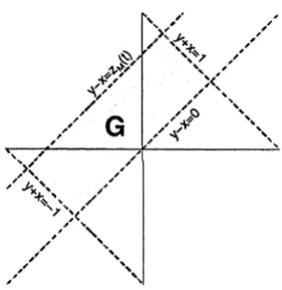
As w is periodic, Z (£, y, t) = Z(a; + L, y + L, t) and so Z is periodic over strips

{ (x, y) : 2nL < y 4- x < 2(n + 1 ) L } .

Figure 3.1: Z is periodic over strips

Within each strip, Z ( y , y , t) = 0 and

Z ( x , y, t) — w(y, t) — u( x, t) — (f> < M — <f) —>0

as \ y - x \ -» oo, so Z attains its spatial maximum in each strip, and hence in the entire plane, for each

t > 0. We can calculate

<t>t = TT <Pt TT» At \ M ’ M 2

J

> j f a W W

and in particular at a maximum point { x , y , t ) with

x ^ y and Z non-negative, equation (3.3) becomes

— < 4a(</>,)</>" - (f)t < 0.

The reason for the restriction x ^ y is that p is not differentiable here. When the maximum is attained at such a point, then Z (x, x, t ) = 0, so in either case Z < 0 for all t. The result follows. □

We can find explicit estimates for more general equations by choosing an explicit barrier.

3.3 Description of a barrier

This barrier, ip, will be used often.

Let $ be the fundamental solution to the heat equation,

so that $ yy = 4c4>*, where c is a positive constant and t > 0. Implicitly define ip(z, t) by

z = 4>(V; — 1, t) — $(ip + 1, t).

This function has the property that as t -> 0,

and (third derivatives are included for completeness but not used until a later chapter) — 1 z < 0.

1 z > 0

and that ^(O, t) = 0 for all t > 0. We can calculate

- M ) - $yW> + M ) ’

r = -

(V,/) 3 [$yyW “ M ) “

W + 1 ,0 ] >

V-'" = 3 ^ / - - M>')4 [$ 9yv(V-- 1 , 0 - ■ W V - + 1,<)],

while

Routine calculations yield

, 2 cy q > y = - ^ e xp

® y y t 3/2

2c 3/5

$ = ^ _ £5/2

2^3/ 2

2qT t

3 -

- 1

+

- 1

2q/J

exp (

-exp exp t erf t erf t

The partial differential equation satisfied by ^ is

(fy _ \_rfrf

dt 4c il)'2

(3-5)

3.4 An explicit estimate for periodic equations

Theorem 3.2. Lef u : R x [0, T ) -> R be a H 2 solution of

ut = a(ux, li, a;, f)wxx + 6(ux)

w(-,0) = wo

where u0 is continuous; both w0 and a are periodic, u0(x + L) = u0(x), a(p ,q ,x,t) = a(p, <7, x + L, f) (and therefore u is also periodic); osc w(-, t) < M ; and where we can find positive constants A and P such that

a(p,q ,x,t)p 2 > A for all \p\ > P. (3.6)

Then there is a T ' > 0 such that fo rt e (0, T'],

|ux| < C \ V t { l + t) exp(C2/t),

where T ', C\ and C2 are dependent on M , A and P.

Proof: Let Z be as before, with <j>(z,t) := 2M'i p{z /2 M, t /^M2) for the ^ defined in Section 3.3, with the constant c given by c = m ax (y ^ -, C P 2) , where C will be chosen later.

Consider the region

where zM {t) satisfies <f>(zM{t),t) = M. Explicitly,

zM {t) = 4 M 2

~7t

Figure 3.2: The (periodic) region G at some time t

As before, Z is periodic over strips parallel to y + x = 0 and so it attains its maximum on G. We first show that Z < 0 on the boundary of G.

For y - x ± 0, as t -» 0, 0 -> 2M and so Z < 0.

At y — x = 0, 0(0, t) = 0 for all t > 0, and so Z( x , x , t) = 0 . At y — x = z m(£)> (f)(zM, t) = M and so Z < 0.

Now suppose that Z attains a maximum on the interior of G.

It follows from (3.3) that at the maximum,

dZ_

dt < 2 [a (c})',u(x,t),x,t) + a (0', u(y, t), y, t)] 0" - 0t

= 2 [a (0', u(x, t),x, t) + a ('ll;', u{y, t), y, t)]

0

0

2M 2a (0', u(x, t), x, t) + 2a (0', u(y, t), y, t)

0t

1 4 c 0 '2 The second derivative

i," = - ( f ) 3 \4,yy{i, - 1, </4JW2) - + 1, t / 4 M 2)]

We can estimate

'ip'2 > inf-i//2 ~ G

>

(

\

sup ^ y { i p — 1, t / \ M 2) — + 1, t / \ M 2)

( K t / K l / 2 '

\ 0< t < T )

- 2

> ( sup sup \$y(l/> - l , t / 4 M 2)| + + l , t / 4 M 2)\ )

\0 < ^< l/2 0< t < V J

> ( SUP $ y (lj> - 1, ?c(V» - l ) 2) + ( ^ + l , | c ( ^ + l ) 2)

\0<V»<l/2 V 6 J \ 6 J

_

(

\0<™Pi/2 (2/3)3/ 2\/c|i/> - 1|2 + (2/3)3/ 2v/c|V>+ 1|2 J

- 2

> C 3352

where the last line follows by choosing C = 3352/(2e3) and recalling that c > C P 2.

Now we can use the condition (3.6), controlling the degeneracy of a, to estimate

dZ ip "

~dt ~ 2 M 2a (ip',u{x, t ) , x , t) + 2a (ip’ ,u(y, i

),

)

<

2M

4A

1 4 cip'2

1 Ac'ip'2

< 0

as c > (16^4)—1. So, Z( < 0 at an internal maximum, Z < 0 on the boundary, and so Z < 0 on G.

Explicitly, for ( x , y , t ) G G, Z < 0 means

U(x , t ) - u ( y j ) < 2 M i ,

< | y —z| s

= \y -

t 3/ 2 { 4 c M 2 \

= l y - x l M 2 M r e x p { ~ ) ’ (3.8)

We can obtain an estimate for (x, y, t ) g G, y > x by observing that for z > zM (t),

u ( y , t) - u ( x , t ) - M z

zM {t) < u ( y , t) — u ( x , t ) — M < 0

so that as \y - x\ > zM {t),

u{y, t) - u ( x , t ) < M \ y — x zM (t)

< I

^ — X 2M 6XP (3.9)

So far, we have estimates for when y > x. We can find identical estimates for the region where y < x by reflecting in the line x - y = 0.

Letting y -> x in the estimates for the difference quotients (3.8) and (3.9) gives the result. □

Comparing p with the special barrier ^ gives us a gradient estimate for solutions of quasilinear equations with this scaling. We will use this estimate in Chapter 5.

C orollary 3.3 (Gradient estimates for the barrier p). L e tp be a smooth solution of

Vt < a(y>',(p,z,t)ip",

on (0,oo) x (0, T ), with the initial and boundary conditions y>{z,0) = 1 fo rt > 0 andz / 0,

y>{0,t) = 0 fo rt > 0,

tp(x, t) —» 1 as x —>oo fo rt > 0.

If

a( p, r, rc, t ) p2 > A > 0 for all \p\ > P > 0,

then there is a V > 0 such that for t e (0, T']

y '( 0, t

) <

+ t)

where T ', C\ and C2 depend on A and P.

Proof: We apply the comparison principle to p and V»e(x,

t)

The barrier dominates p on (0 ,00) x {0 } and {0} x [0, T].

Then P p = - p t + a ( p ', </?, z, t ) p " > 0 and

P'lpe = — e — 'ipt + x i t ) ^ ’

v/

W)

so Theorem 2.1 implies that ^ > y? on (0,zi) x (0,T') for all e > 0, and as e -> 0, V>° > y?. Since V>°(0, t) = ip(Q, t) this gives us the boundary gradient estimate

y/(0, £) < V;/(0, t / 4) < C i ^ ( l + £) exp (C^/f).

□

3.5 Interior estimates for non-periodic equations with 6 = 0

Theorem 3.4. Let u : ^ x [0, T] -» R be a H 2 solution to

Ut riipixi ü, x, t^Uxx 5

where Q c t is an open interval and where there are positive constants A and P so that

a(p, q, x ,t)p 2 > A for all \p\ > P. (3.10)

If oscnx[0 Tj u < M, then we can find an estimate for 0 < t < T

\u \x , t )| < C \V t{\ + t) exp ’

where T ’ , C\ andC 2 are dependent on A, P, M and dist(rr, dfl).

We modify the previous proof, introducing a new boundary in the x, y coordinates, since we no longer have compactness of the domain through periodicity. We will seek to avoid a maximum of Z occurring on the new boundary.

Proof: Firstly, suppose that Ü = (-1 ,1 ). We consider the sub-region

G := { { x , y , t ) e ( - 1 , l ) 2 x [0,T'] : 0 < t < T 1 < T, \y + x\ < 1,0 < y - x < zM {t) },

Define Z on G by

Z ( x , y , t ) := u{ y , t ) - u ( x , t ) - ß ( x , y , t ) .

In order to avoid a positive maximum of Z on the boundary, we will ensure that 0 satisfies

• (f)(x, y, 0) > M for y ^ x

• <t>(x, y, t ) > M for \y - x\ = zM { t)

• 0(x, x, t) > 0for t > 0

• (j)(x, y , t ) > M for \y + x\ = 1.

where -0 is the explicit barrier defined in Section 3.3, for positive constants c and 7. We will also choose ß with \ß\ < 1 / 2 later.

This 0 satisfies the first three conditions. In order to fulfill the final condition, choose 7 = M / ( 1 - 2\ß\)2. Then at \x + y\ = 1,

Figure 3.3: The region G at some time t

We choose

^ + l ( x + y - 2ß)2,

Now suppose that Z first reaches a positive maximum at an internal point (re, y, t) e G. As usual, we calculate that at this point first derivatives are zero

0 = Zx = —u'(x, t) + ip' — 2/y(x + y— 2/3), 0 = Zy = u'(y, t) - i l) ' - 2 7(2: + y - 2/3),

and the matrix of second derivatives is negative semi-definite

ZxX _{____}_

1

- u " ( x , t )- - 27 _{mr- 27}

1

-N _{'S Z y y}

m

r

We use these in the evolution equation for Z

— = a(uy, u(y), y, t ) u yy - a(ux, u ( x ) , x , t ) u xx - <J)t

a{uy, u ( y ) , y , t ) 'll)"

z «y + 2m + 2 7 tpt

- a (ux , u ( x ) , x , t ) — Z Xxxx ---272 M 'll)" r

- 7T77 “ (a(wy> 0 + a(wx, w(x), x, £)) Zxy

( f _ _

2 M

+ (a(uy, u(y), y, f) + a(ux, itfa), x, £))

V2M 27

— trace ( a(ux , u { x ) , x , t ) - a ( u Xi u { x ) , x , t ) Zxx Z xy l - a { u y, u ( y ) , y , t ) a{uy, it(y), y, t) ZyX Zyy

ip"

+ 2a(uy, u ( y ) , y , t ) —— + 2a{ux , u ( x ) , x , t)

<

2M

2a(uy, u(y), y , £) + 2a(ux, u(x), a;, £)

2 M 2 M 1

4 cip' 'iP"

2M ’

the last line applying at the internal maximum. As before, ip" < 0 for t < T < 2cM 2/3. The first derivative condition for Z implies that ux = ip' - 2 7(2: + y - 2/3) and

+ 27(2: + y - 2ß) and so

max(|ux|, |i4y|) > \ip'\ > P, (3.11)

where the final inequality comes from choosing c > C P 2 as in the previous section.

We can then exploit (3.10), the condition on a;

2A 2a (uy, u(y), y, i) + 2a (ux, 11(2;), 2;, f) >

>

max (|ux|, |ity|)' 2 A

{\ip'\ + 27I2: + y — 2/3|) 2 •

bound on l^'l, and choose

(47 + P)2

c >

8 AP2

4M \ 2

+ P ) 1

(1 - 2|/3|)2 y 8AF2

Now < 0 at interior maxima, and so the parabolic maximum principle ensures that Z < 0 on G.

For points outside G, but in the rectangle \y + x\ < 1, ZM(t) < y - x < 1,

u{y, t) — u(x, t) < M < M\y - s| zM{t)

< f t

S M ? " P

We can repeat both these estimates for a reflected region where x > y, putting them all together gives

/ \ , \ I _ ,, , / \y — x\ t \ M i x — y ) 2 \ / t ( c M 2 \ .

|u(x, t)- u ( y,<)| < 2Mip^ J + (1 _ 21,31)2 + exP ( — ) |y

Now, for \y\ < 1/2, set ß = y and let x y to give a gradient estimate at y

. . . .. , / t \ v 7 ( cM 2 \

^ exP

- xl.

t3/ 2

( r r )

\Jt ( cM

+ 2 M eXP

2 s

For the case of a general interval Q = [xi, ar2]. we can rescale around a point y e Q by using scaled coordinates x = 2(x - y)/dist(y,dQ). We obtain the estimate

\u'(y,t)I <

dist(y, dfl)

where c depends on A, P, M, and dist(y, dQ). □

t3/ 2 / 4cM2 \ w r ( cM2 \

2 i Ö P eXP{ — ) + M V i e X P { — )

3.6 A generalisation to fully nonlinear equations

In this section we consider equations of the form

ut = F(uxx, ux, u, x, t), (3.12)

Let u be a smooth solution to (3.12). As before, define

Z ( x , y, t) := u { y , t ) - u { x , t) - (f>(\y - x\ , t) ,

and suppose it first becomes non-negative at some point (x, y, t), with y > x. First and second derivatives of Z will satisfy (3.1) and (3.2), but the evolution equation for Z will be given by

d Z

— = u t ( y, t) - ut {x, t) -

Ml

= F ( u yy,Uy, u ( y ) , y, t) - F(uxx, ux , u { x ) , x , t)

- M\y - x\,

= J — {suyy + (1 - s)uxx,siLy + (1 - s)ux ,su(y) + (1 - s ) u ( x ) , s y + (1 - s) x, t) ds

- M \ y - x\,t)

r l d F

} J (SUyy + (1 - S)UXX, . . .) dS

) ds — [U y y U

= trace a ci

C2 a

. r1 dF

(■SUyy

S)UXX,

dS

U y - 1* x ] /

Jo dp

M y )

r l _dF

- u { x ) \ Jo

q (SUyy “I“ (1 ^ H ' X X l • • •

y - x J r l d F

— {SUyy

Zxx

Zyx

-Zxy

Zyy_

\ r 1 Q j ?

J F 2(f) J^ (

SUyy

d F

~ (c i + c2)</>" - <f>t + (f) J (S U y y + (1 - s)uxx, . . . ) ds

r l d F

+ [y - x\

j —

where we have used that u y= u xat a spatial maximum, and have abbreviated

d F

J — {suyy + (1 - s ) uxx, . ..) ds = a

and where we have added and subtracted (ci + c2) Z xyfor some clf c2. If we choose

Cl — C2 — ~ a

is negative semi-definite, we have

dZ_

dt < 40"

dF_

d r ( S Uy y + ( 1 - S ) U1 . . ) ds - (f)t

+ 0

dF_

dq (suyy4* (1 s'j'Uxxi • • •) ds

+

dx + (1 - s)uxx, . . . ) ds.

If we make quite harsh restrictions on F, then we can use our explicit barrier to find an analogue of Theorem 3.2 for periodic nonlinear equations.

Theorem 3.5 (Nonlinear version of Theorem 3.2). Let u : R x (0,T ) -4 IR be a C 2 solution of

Ut — F ( u xx, ux , u, t)

u ( - , 0) = u0

where u0 is continuous and periodic, u0(x + L) = uq{x), (and therefore u is also peri­ odic); osc u(-, t) < M ; where we can find positive constants A and P such that

d F

~ ^ {r,P ,q ,t)p 2 > A for all \p\ > P;

and where —— < 0 . dq

Then there is a V > 0 such that fo rt e (0, T %

|itx | < C i V t ( l + t) e x p (C 2/ f ) ,

where T , C\ a n d Ö2 are dependent on M , A and P.

Proof: The proof is the same as that of Theorem 3.2, including the choice (f){z,t) = 2 M 0 (z/2 M , t / A M 2), but instead of using inequality (3.3) for interior maximum points, we have

dZ_

dt _Jo

f

d F

/„

~ t (

f

Accf)'2

< 0,

where the omitted argument of the derivatives of P, denoted by ( .. . ) , is (suyy + (1 -

An existence result for a parabolic

equation in one space dimension

Although this is a standard result (see Theorem 12.25 of [25]), for completeness we sketch a short time existence result in the one-dimensional case, where the spatial domain is Q = (z q, xi ) c R and the initial and boundary data is continuous.

The parabolic equation is

l i t — Q , { u x , U , X ^ t^ U x x t (4.1) with initial and boundary data prescribed by

u ( x , t) = uo( x,t ) for (x , t) 6 x [0,T]). (4.2)

We require that a > 0 is in H a (K) for all bounded i C C M x M x f i x [ 0 , T ] and some a £ (0,1).

This implies that for every such /C we can find positive Xjc and Kjc such that Ajt < a(p,«?, a;, t) < A/c, when ( p , q , x , t ) e /C. (4.3)

When we can find bounds of this type that depend only on the gradient, we will write

\ { K ) < a { p , q , x , t ) < A ( K ) , for \p\ < K . (4.4)

Suppose also that there are positive constants A and P such that

a(p, g, x, t )p2 > A > 0, for \p\ > P. (4.5)

The first part of this chapter is a survey of the main steps needed to find the

tence result for the Cauchy-Dirichlet problem with H1+jg initial and boundary data. We

follow the treatment in Lieberman [25].

These results mean that when we approximate continuous initial data by smooth initial data, a solution will exist for the approximate initial data. In the later parts of the chapter, we use the gradient estimate established in Chapter 3 to find uniform gradient estimates for t > 0. This will gives us a solution for t > 0; in order to show that this approaches the initial data as t ->• 0, we will need some displacement estimates which limit the distance a function can travel in a given time.

4.1

Existence of solutions with

H 1+ß

initial and boundary

data

Theorem 4.1. Consider the Cauchy-Dirichlet problem given by (4.1) and (4.2), where

0 <

ß

< 1.

Suppose that u0 is defined on the parabolic boundary ? ( H x [0,T ]) and u0 e H i+ß(V). Also, suppose that either u0 is time-independent, or else there are con­ stants A and P such that (4.5) is satisfied.

Then there is a smooth solution u e C2+l (Q x (0, T)) n C ( f l x [0, T ] ) .

This solution has a gradient bound\u\x+^ 5/ 2 < C where C depends on \u0\l+ ßß/2,

ß, \)c, Ak a n ddiamQ.

The proof of this result follows a standard pattern for showing existence — a bound on sup |it|; a bound on sup\Du[, a Holder gradient bound \Du\a\ and then the applica­ tion of a fixed point theorem. These steps are sketched by the following results.

We begin by using the comparison principle to bound \u\.

Lemma 4.2 (A bound on sup \u\). Ifu is a smooth solution of (4.1), (4.2) in Q x [0, T], then

sup |u(x, £)| < sup \uq\.

Qx[ 0, T]

Proof idea: Set k = sup u0+ and apply the comparison principle (Theorem 2.1) to u and k on E := { (x, t) G f i x [0, T] : u(x, t) > 0 }. Since k > u on dE, it follows that k > u on all of E and so on all of f i x [0, T].

Similar steps can be followed to find that in ffix [0 T]U > in fu 0~ , completing the result. □

We begin our gradient estimates with a boundary gradient estimate.

condition (4.5), then

\ u( x, t ) - u( y, s) \ ^ T

SUP —7~,---r---tt— ^ L i

(x,£)£<9Qx[0,T] — ( 2 / i s )l

( y , s ) e ü x [ 0 , t ]

where L depends only on osc uq, \u0\1+ßß/2and ß .

In fact, we can relax the regularity requirements on the initial and boundary data and still find a continuity estimate on the boundary.

A modulus of continuity is a concave, continuous function u : M+ -» R+ , with w(0) = 0. This a; is a modulus of continuity for a function g at y if

19(x) - g(y)\ < u(\x - y|)

for all x in the domain of g. It is a modulus of continuity for g if the above relationship also holds for all y in the domain of g.

A modulus of continuity can be defined for every continuous function on a closed bounded set.

Lemma 4.4 (Boundary continuity estimate). Let u satisfy (4.1), (4.2), where uq has

modulus of continuity u>, and suppose there are positive constants g and P so that

\p\A(p, q,x,t) + 1 < ga{p, q, x, t)p2 (4.6)

whenever \p\ > P.

Then u has a modulus of continuity on the boundary

\u{x,t) - u {y ,t)I < u*(\x - y |)

forx £ Q andy e d t t , where u>* can be determined by w, supp |u0|, EL, and a.

Equipped with the boundary gradient estimate, we can now find a global gradient estimate. In this one-dimensional case, the global gradient estimate is the result of Kruzkov mentioned in Chapter 3.

Lemma 4.5 (Global gradient estimate). If u is a smooth solution of (4.1), (4.2) in EL x [0, T] with an oscillation boundosc u = M , and a Lipschitz estimate on the parabolic boundary\u(x,t) - u(y,t)\ < L\x - y\ for all (x ,t) e V{EL x [0 ,T ]) andy e EL, then

sup iu x \ < 2L . nx[o,T]

(p, q, x, t) in the set JC := { (p, g, a:, £) : |p| < if , |g| < M , x € Q , t e [0, T ] },

Ajc < a ( p , q , x , t ) < Ajc

-I f u e C2+1(ft x [0,T]) n C ( n x [0, T]), set M = supM and K = sup|D«|. Then there are positive constants a andC determined by ß, Xjc, Ak. and d ia m fi such that

[Du\a < C (sup |w| + s u p\Du\ + |« o |i+jg>/3/2) •

Now that we have bounds for M 1+Q Q/ 2, we can apply the following existence the­ orem, which is derived from a fixed point theorem.

Lemma 4.7 (Existence theorem). Let u0 be in H i+s for some S e (0,1)

If there is a constant independent of e such that any solution of (4.1), (4.2) on

Q x [0, e) satisfies

\u \l+6,S/2

< Afj,

then there is a solution of the Cauchy-Dirichlet problem (4.1), (4.2) in Q x [0, T\.

4.2 Displacement estimates

The following estimates for the displacement suffered in a given interval of time by a function moving under a parabolic flow apply to any strictly parabolic operator satisfy­ ing bounds of the form (4.3) or (4.4).

Lemma 4.8 (Displacement estimate for Lipschitz initial data). Letu : Q x [0, T] -* R satisfy (4.1), where fiC M , and a has bounds of the form (4.4).

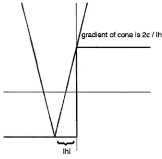
Suppose that u has initial data whose graph lies below a cone centred at some point h

u ( x, 0) < L \ x — h\

and, in the case that tt ± R, whose boundary data lies below the same cone

u ( x , t ) < L \ x — hI, x € dQ.

Then, at later times,

u ( x , t ) < L { x — h)Evi {x ~ h)2\

AM ) ’

(4.7)

Proof: For some small e > 0, set

v ( x , t ) \ = L { x — h)Sxi

+

t + e /

which satisfies the heat equation

and approaches the cone of gradient L centred at h as t + e ->> 0.

Figure 4.1: The barrier v(-, t)

Note that v ( x ,0 ) > L \ x — h\, that \vx ( x, t) \ = L £ rf { x y j c / (t + e)^

^i i ^ 0, so

< L and that

vt - a(vx , v, x , t ) v xx > v t - sup a{p, v, x, t ) v xx

\ P \< L

> v t - A [ L ) v xx

= 0

where we choose c~l = 4A(L).

The estimate follows by applying the comparison principle (Theorem 2.2) to show that u(:r, t) < v(x, t), and then letting e 0.

□

Now, we apply this to three different cases, firstly when u initially satisfies a Holder condition and when we have polynomial growth in A, secondly when u(-,0) has a modulus of continuity, and thirdly when u is initially bounded by a step function.

polynomial growth, so that

a(p, q, x, t) <

A(1 + K m)

where Ä and m are positive constants. Also, suppose that u(-,0) satisfies a Holder condition around some point h

|ii(/i, 0) — w(x,0)| < L\x - h\a, 0 < a < 1.

Then, at later times,

Iu(h: 0) — u(h: £)| < c(o;, m, L, K ) t2+r"(1- “ ) .

Proof: For simplicity, assume h — 0 and u(h, 0) = 0. The initial data is bounded

\ \ \

Figure 4.2: The bounding cusp is itself bounded above by cones

above by cones centred at h and indexed by k, the (positive) ^-coordinate of the point of contact with the bounding cusp L|:r|Q, so

u(x, 0) < L\x\a < a L k a~l \x\ + L( 1 — a)ka.

The estimate (4.7) taken at x = 0 is then

u(0,f) < 2L a k a~l (1 + (LkQ- l ) m) l/2 y j ^ - + L{ 1 - a)ka

and optimizing over k gives

u(0, t ) < c(a, m, L, A ) i2+m(1_Q) .

□

continuity u at a point h

u(h, 0) — u(:r, 0)| < u (\x — h \ ) .

Then

|u(/i,0) — u(h,t)\ < c(t)

where c is dependent on u andA, and where c(t) ->• 0 as t -> 0.

Proof: For simplicity, assume h = 0 and u(h, 0) = 0. Consider the cones

Ck(x) = ck (|x| - k) + uj(k)

indexed by k > 0, the (positive) z-coordinate of a point of contact with u. As u is concave it has both left and right derivatives, and we can choose the slope of the cone ck = uj'_(k). Then

u (x ,0) = n(x,0) — u(0,0) < a>(|a:|) < <jj'_(k) (|x| — k) + cu(k) = Ck(x).

Now we have a cone as an upper boundary, we can use estimate (4.7) at x = 0

where A = A(u'_(k)) is given by (4.4). Minimize this over k to get the displacement bound

In order to show that c(t) -* 0 as t -> 0, let 6 > 0. As u is concave and positive, it has positive left derivative and for k > 0 we have

u(0,t) < 2u’_(k) — uj'_{k)k + cv(/c),

0 < cj'_(k)k < cj(k).

And as u is continuous,

0 < lim u ' [ k ) k < lim u(k) = 0.

“ f c—>0 _ k^>0

Choose k = ks so that uj(k0) - uj'_(ks)k6 < 6. Choose r so that

{u'_(ks))

then for all t < t,

c(t) < 2 — u)'_(ks)ks 4- uj(ks) < 26,

and so c(t) 0. □

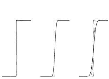
Set a to be the maximal monotone graph

cr(x) --- <

which we will refer to as the step “function”.

+1? x > 0

[-1.1], x — 0 (4.9)

-1 , x < 0

Corollary 4.11 (Displacement estimate for step functions). If u satisfies (4.1) and (4.4), and is initially bounded by a step function

then for x < 0

u ( x, 0) < ccr(x),

. . . I 4c At u ( x, t) < mm < —- \ ---c, c

X V 7T

where A = A(2c/|ac|) as in (4.4).

Proof: Near some point h < 0, u(-, 0) satisfies a Lipschitz condition

u(o:,0) < L h\x— h\ — c

where L h = 2c/\h\.

Lemma 4.8 then gives that

u ( x , t) < inf r ^rSrf f — 7 = ) h< 0\h\ \ 2 y / k t )

4c / At

+ 777 A/ — exP

(a: — h)‘

4At — c

and if we let h — xthen we find that for x < 0,

u ( x , t) <

_v

~ \ \ — c

-X V 7T

gradient of cone is 2c / Ihl

Figure 4.3: Cone bounding the step function

Remark: If a satisfies the condition (4.8), then

u ( x , t ) < C ( c , A ) c1+m/2V i | x r1- m / 2 - c .

□

4.3 Existence of solutions with continuous initial data

Theorem 4.12. Consider the Cauchy-Dirichlet problem given by (4.1) and (4.2). If

uqg C (V(Q x [0, T])) and if there are constants A and P such that (4.5) holds, then (4.1), (4.2) has a solution u e

C2+1

n C

The first step in the proof of the above is to approximate u0by ue0 in C°°, so that suPxen lwo ~ u 0\ < e .

Lemma 4.13 (Existence of solutions with approximate boundary data). For all

e > 0, there exist solutions ue : Et x [0,T] -» R to (4.1) with boundary data ue0 These solutions are in C 2+l (ft x [0, T])

n C ( Ü x

Proof: As ue0 is in the Holder space Hi+ß, this is a consequence of Theorem 4.1. □

Lemma 4.14 (Existence of uniform oscillation bound). For all e > 0,

osc u€ < 4 (sup |uo|).

follows that k > ueon all of E and hence on all of Q x [0, T], and so

sup Iue(x, t)\ < sup |uq| < 2 (sup \uq\ ) ,

Q x[0 ,T ]

where the last inequality will hold for small enough e.

This leads to a uniform oscillation bound for ue,which we denote by M —

osc ue < 4sup|uo| = : M.

□

Theorem 3.4 gives a uniform gradient bound on interior sets, up to some time r > 0. For to

e

\uex\n'x{t0,T') < C\y/tö{l + ^ o )e x p = : L(to),

where T , C\ and C2are dependent on A, P, M and dist(Q ', dft).

Lemma 4.15 (Higher regularity on interior sets). On interior sets Ü' x (2t 0, T' ) we can estimate higher derivatives

\ue\2+k+a < C

where C depends ondist(Q ', dtt), diam (Q ), to, A, P, |a|Q and M .

Proof: Once we have an oscillation bound M and a gradient bound L ( t 0), (4.3) im­ plies uniform parabolicity. A uniform Holder gradient bound on interior sets results from Theorem 12.2 of [25]. In particular, on interior sets and when T' /2 > t Q > 0,

W ex \ a - , n ' x ( 2 t 0,T') < C 'm in { d is t ( f i', ö Q ) , v / ^ } “ Q ,

where both a and C depend on A % and A^, given by (4.3), with

/C = { (p , q, x, t) : |p | < L(to), \q\ < M , x G Q , and t e [0, T ] } and C also depends on L(to) + M , and diamS2.

Equipped with a Holder gradient bound, we can treat the equation as a uniformly parabolic equation with Holder continuous coefficients, and use standard results, such as Theorem A .4, to find that ue is uniformly bounded in H 2+a (JV x (2f 0, T')).

From here, it is possible to use the bootstrapping method to obtain interior esti­ mates for all higher derivatives.

□

In order for this u to be a solution of the Cauchy-Dirichlet problem, we need to show that u attains the initial and boundary data.

Lemma 4.17 (Convergence to initial data). On any spatially interior set f t ' ,

sup |u(x,t) — uo(a^)| —> 0 as t —> 0. xEQ'

Proof: Let x be any point in ft'. Let u be a modulus of continuity for u0. We can off-set ue by defining

we(y, t) := ue(y, t) - ue(x, 0) + u0{x),

so that we(x, 0) = uo(x). Let u be the limit of a subsequence ue, as in Corollary 4.16.

|u(x, t) — uo(^)| = lim \ue{x, t) — uo(x)| £—>■0

= lim \we(x, t) + ufc(x ,0) - 2uo(x)| e—>0

< lim ( | ^ e(m, t) - uq(x)\ + Iue(x,0) — ito(^)l) £->0

= lim |we(x, t) — we(x,0)| + lim \ue(x,0) — ito(x)|.

e->0 e—>0

The second of these terms is zero. To estimate the first term, note that the approxi­ mations ue(-, 0) satisfy the same the same continuity condition as u0, and therefore so does u»e(-,0), with |^ e(0, m) - w €(0, y)\ < u ( \ x - y \ ) , for all x , y e f t . Corollary 4.10 then gives the estimate

|we(x, t) — we(x, 0)| < c(i),

where c depends only on the exact forms of u and Ajc (given in (4.3)). In particular, c is independent of x and e, and as c(t) -> 0 as t ->• 0, the result follows. □

More specific continuity-in-time estimates are given by the continuity of the initial data and the upper growth bound of a. If, for example, the initial data is Holder contin­ uous

N M - u0(y)\ < L\x - y\a

and a has polynomial growth in the gradient term, satisfying (4.8) for constants Ä and m, then Corollary 4.9 indicates that c(t) = C(a, m, L, Ä) \t\2+«*o-«).

Lemma 4.18 (Convergence to boundary data). We can continuously extend u(-, t),

defined on the interior of ft at time t, to ft. Moreover, u = u0 on the boundary.

We note that our parabolic equation satisfies condition (4.6), since

2 \p\A{p,q,x) + 1 = \ p\ \ a{p, q, x)\ + 1 < ^ a |p |2

for \p\ > P, using (4.5).

Let a; be a modulus of continuity for u0. As each ue0 has at least the same modulus of continuity as u0, Lemma 4.4 gives us an estimate uniform in t and e,

Iue(x,t) - ue0(y,t)\ < uj* ( \x - y\). Then for a point y e dQ and fixed t,

sup \u{x,t) - U0{y,t)\ = sup I Yimue{x,t) - ue0{y,t) + ue0(y,t) - u0(y,t)\

Br (y)nn Br (y)nn €^ °

< sup UJ* (|x - y\)

Br { y) no

= w*(r)

so as \ x - y \ -> 0, u*(\x — 2/|) —> 0 and u{x, t) -* w0(y, t) — that is, we can continuously extend u to u0 on dCl for t > 0. □

4.4 Existence of entire solutions with stepped initial condi­

tions

Consider equation (4.1), under the conditions on a given by (4.3) and (4.5).

Lemma 4.19. There exist entire solutions to this equation with the periodic, crenellated initial data

gR(x) = Mg (sin(irx/R) ) , where g is given by (4.9).

Proof: If we let g€ be the smooth mollification of gR, then for |a;| < R,

Theorem 4.1 ensures that there is a smooth solution u eto 4.1 with initial condition g£, with a Holder gradient bound dependent on e. The gradient bound in Theorem 3.2 is independent of e; for t e (0, T'),

\uex \ < C \ V t ( l + t) exp{C2/ t )

where T', C\ and C2are dependent on M , A and P, but not R. Higher gradient bounds for t > 0 follow from the interior estimate (4.15) and we can find a subsequence converging to u Rwhich also solves the equation on [t,T'].

To show convergence of u Rto the initial data, suppose that - R / 2 < x < 0. As in Section 4.2, we can bound the initial data geby cones centred at h e { - R / 2 , - e ) —

9\x)<JP\X-h\-M.

Applying Lemma 4.8 to this, and setting h — x , w e find that for - R / 2 < x < -e,

u€( x , t) <

where A = A { M / \ x + e|) as in (4.3) and so we have the estimate

|u R{ x,t ) - gR{x)\ = | lim ue(x, t) + M\

A similar estimate holds for all x ^ nR, and so for all g > 0, we can find t (dependent on x) such that |uR{x,t) - gR{x)\ < g. □

Corollary 4.20. There exists an entire solution to this problem with the initial data

uo(x) = Mct(x).

This solution has a gradient estimate fo rt < T :

\ux \ < C \ y / t ( l + t) exp{C2/t),

where V , C\ andC 2 are dependent on M , A and P.