Computation
.
White Rose Research Online URL for this paper:
http://eprints.whiterose.ac.uk/106038/
Version: Accepted Version
Proceedings Paper:
Carr, HA, Weber, GH, Sewell, CM et al. (1 more author) (2017) Parallel Peak Pruning for
Scalable SMP Contour Tree Computation. In: 6th IEEE Symposium on Large Data
Analysis and Visualization. LDAV 2016, 23-28 Oct 2016, Baltimore, MD, USA. IEEE , pp.
75-84. ISBN 978-1-5090-5659-0
https://doi.org/10.1109/LDAV.2016.7874312
© 2016 IEEE. Personal use of this material is permitted. Permission from IEEE must be
obtained for all other uses, in any current or future media, including reprinting/republishing
this material for advertising or promotional purposes, creating new collective works, for
resale or redistribution to servers or lists, or reuse of any copyrighted component of this
work in other works.
[email protected]
https://eprints.whiterose.ac.uk/
Reuse
Items deposited in White Rose Research Online are protected by copyright, with all rights reserved unless
indicated otherwise. They may be downloaded and/or printed for private study, or other acts as permitted by
national copyright laws. The publisher or other rights holders may allow further reproduction and re-use of
the full text version. This is indicated by the licence information on the White Rose Research Online record
for the item.
Takedown
If you consider content in White Rose Research Online to be in breach of UK law, please notify us by
Parallel Peak Pruning for Scalable SMP Contour Tree Computation
Hamish A. Carr∗
University of Leeds
Gunther H. Weber†
Lawrence Berkeley National Laboratory University of California, Davis
Christopher M. Sewell‡ James P. Ahrens§
Los Alamos National Laboratory
ABSTRACT
As data sets grow to exascale, automated data analysis and visu-alisation are increasingly important, to intermediate human under-standing and to reduce demands on disk storage viain situ anal-ysis. Trends in architecture of high performance computing sys-tems necessitate analysis algorithms to make effective use of com-binations of massively multicore and distributed systems. One of the principal analytic tools is the contour tree, which analyses rela-tionships between contours to identify features of more than local importance. Unfortunately, the predominant algorithms for com-puting the contour tree are explicitly serial, and founded on serial metaphors, which has limited the scalability of this form of analy-sis. While there is some work on distributed contour tree computa-tion, and separately on hybrid GPU-CPU computacomputa-tion, there is no efficient algorithm with strong formal guarantees on performance allied with fast practical performance. We report the first shared SMP algorithm for fully parallel contour tree computation, with for-mal guarantees ofO(lgnlgt)parallel steps andO(nlgn)work, and implementations with up to 10×parallel speed up in OpenMP and up to 50×speed up in NVIDIA Thrust.
Keywords: topological analysis, contour tree, merge tree, data parallel algorithms
Index Terms: I.3.5 [Computer Graphics]: Computational Geom-etry and Object Modeling—Curve, surface, solid, and object rep-resentations I.6.6 [Simulation and Modeling]: Simulation Output Analysis;
1 INTRODUCTION
Modern computational science and engineering depend heavily on ever-larger simulations of physical phenomena. Accommodat-ing the computational demands of these simulations is a major driver for hardware advances, and has led to clusters with hun-dreds of thousands of cores to achieve petaflops of performance and petabytes of data storage as well as the effort to achieve sus-tainable exaflop performance within the next seven to nine years. For recent hardware, the I/O cost of data storage and movement dominates, and increasingly requiresin situdata analysis and vi-sualisation, increasing the appeal of algorithms that can efficiently and automatically identify key features such as contours while the simulation is running, and store only those features to disk, rather than all the raw data. Whilein situanalysis requires distributed al-gorithms, with clusters now built around NVIDIA’s Tesla cards and Intel’s Xeon Phi boards, we are seeing a return of SIMD (Single In-struction, Multiple Data) computational models for shared-memory architectures, and algorithms will need to exploit this.
In situanalysis and visualisation require more sophisticated ana-lytic tools—to identify relevant features for further analysis and/or
∗Email: [email protected]
†Email: [email protected] ‡Email: [email protected] §Email: [email protected]
output to disk—as does the recognition that one component of the pipeline remains unchanged: the human perceptual system. This need has stimulated research into areas such as computational topology, which constructs models of the mathematical structure of the data for the purposes of analysis and visualisation. One of the principal mathematical tools is thecontour treeorReeb graph, which summarizes the development of contours in the data set as the isovalue varies. Since contours are a key element of most visu-alisations, the contour tree and the relatedmerge treeare of prime interest in automated analysis of massive data sets.
The value of these computations has been limited by the algo-rithms available. While there is a well-established algorithm [7] for computing merge trees and contour trees, the picture is patchier for distributed and data-parallel algorithms. While some approaches exist, they either target a distributed model [1], or have serial sec-tions [16], do not come with strong formal guarantees on perfor-mance, and do not report methods for augmenting the contour tree with regular vertices, which is required for secondary computations such as geometric measures [8]. We therefore report a pure data-parallel algorithm with strong formal guarantees and practical run-time, that computes either the merge tree or the contour tree, aug-mented by any arbitrary number of regular vertices.
2 BACKGROUND
Since the goal of this work is to use data-parallel computation to construct an algorithm for contour tree computation, we split rel-evant prior work between data-parallel computation (Section 2.1) and contour tree computation (Section 2.2). This divide is not strict, since some work has been published on distributed and parallel con-tour tree computation, but is convenient for the sake of clarity.
2.1 Data-Parallel Computation
Data-parallelism is one effective method for exploiting the shared-memory parallelism available on accelerators, such as GPUs and multi-core CPUs. Blelloch [3] defined a scan vector model and showed that many algorithms in computational geometry, graph theory, and numerical computation can be implemented using a small set of “primitives.” These primitive operators—such as trans-form, reduce, and scan—can each be implemented in a constant or logarithmic number of parallel steps. NVIDIA’s open-source Thrust library provides an STL-like interface for such primitive op-erators, with backends for CUDA, OpenMP, Intel TBB, and serial STL. An algorithm written using this model can utilize this abstrac-tion to run portably across all supported multi-core and many-core backends, with the architecture-specific optimisations isolated to the implementations of the data-parallel primitives in the backends. PISTON [15] and VTK-m use Thrust for algorithms such as isosurfaces, cut surfaces, thresholds, Kd-trees [23] and halo find-ers [11]. Halo finding [11, 22] makes use of a data-parallel union-find algorithm, which most contour tree algorithms depend on.
(a)
24
15 22
10 13
0
(b)
24
15
10
1 8
0
(c)
24
15 22
10
1 13
8
0 6.5 11.5 21.25
(d)
24
15 22
10
1 13
8
0 6.5 11.5 21.25
(e)
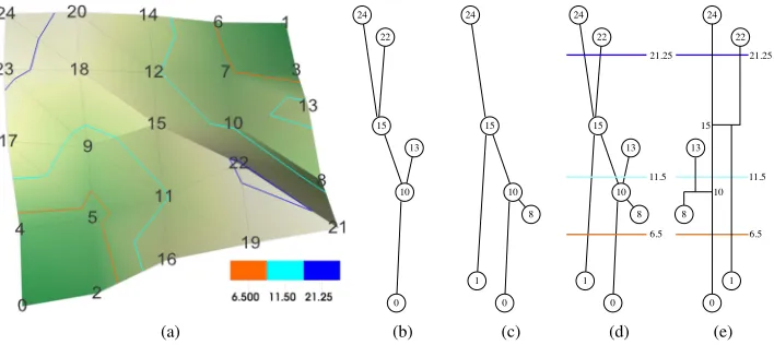
Figure 1: (a) Landscape and select isolines. (b), (c) Join and split tree record where maxima and minima respectively “meet.” (d) The branch decomposition is a hierarchical representation of the contour tree based on a simplification measure.
2.2 Contour Tree Computation
A considerable literature has now built up on the contour tree, its algorithms and its applications. We give some definitions and then canvass the algorithmic papers relevant to our new approach.
2.2.1 Contour Tree Definition
Given a function of the form f :Rd →R, a level set—usually termedisosurfacein scientific visualization—is the inverse image f−1(h)of anisovalue h, and acontouris a single connected
com-ponent of a level set. TheReeb graphis obtained by contracting each contour to a single point [21], and is well defined for Eu-clidean spaces or for general manifolds. The number and, in three dimensions, the genus of contours changes only at isolatedcritical points. Critical points where the number of contours changes ap-pear as nodes in the Reeb graph. For simple domains, the graph is guaranteed to be a tree, and is called thecontour tree.
The contour tree abstracts isosurface behavior, as seen in Figure 1. By contracting contours to single points, it indexes all possible contours. If the contour tree is laid out so that they-coordinates correspond to function value (Figure 1), a horizontal cut intersects one edge of the contour tree per connected isosurface component at the corresponding isovalue. We show three such cuts: orange at 6.5 (two contours), cyan at 11.5 (three contours) and blue at 21.25 (4 contours). This property was exploited in one of the early visual-ization applications: accelerated extraction by generating seed cells for isosurface extraction by contour following [26, 27].
As well as relating contours and critical points, contour trees also allow assigning importance to features [8] and ignoring features below an importance threshold. Features are defined by pairs of critical points, usually an extremum-saddle pair. The most common pairing is throughtopological persistence, shown in Figure 1.
At saddle 15, peaks 24 and 22 meet, and we pair one with 15: the choice can be based on isovalues or on geometric properties of the peak [8]. Here, peak 24 has higher persistence (24−15=9) than peak 22 does 22−15=7), so 22 pairs with 15 and is subor-dinate to peak 24. 24 is now a single peak with saddle at 10: this is more persistent than peak 13 (13−10<24−10), and peak 24 is ultimately paired with the minimum at 0. This process, applied to all critical points, results in the hierarchicalbranch decomposition of Pascucci et al. [20], shown in Figure 1(e).
Instead of these pairs orcancellations, we can assign each crit-ical point to itsgoverningsaddle, i.e. the saddle at which it joins another peak. In Figure 1, 15 is the governing saddle forboth24
and 22, and 10 is the governing saddle for both 13 and 15 - i.e. we can assign governing saddles to saddles themselves.
Whether we use cancellation or pairing with governing saddles, simplification of the tree then consists of cancelling the extremum with the saddle, e.g., by “flattening” it, chopping off the correspond-ing peak or “fillcorrespond-ing in” the correspondcorrespond-ing valley.
For data analysis, we normally assume that the domain is a mesh—i.e., a tessellated subvolume ofRd, such as is used for
nu-merical simulation. For simplicial meshes in particular, all criti-cal points of the function are guaranteed to be at vertices of the mesh [2], massively simplifying topological computations.
We will refer to the number of vertices in a graph asV and the number of edges asE, and note that pathological tetrahedral meshes may haveE=Θ(V2). For regular meshes (our principal targets at present),E=Θ(V). In all practical cases, however,V<E.
In practice, the contour tree may also beaugmentedby regular points, which is important if geometric computations are to be per-formed over the tree for analysis or visualisation purposes.
2.2.2 Sweep And Merge Algorithm for Contour Trees For simplicial meshes on simple domains, thesweep and merge algorithm [7] performs a sorted sweep through the data, incremen-tally adding all vertices to a union-find data structure [25]. As com-ponents are created or merged in the union-find, critical points are identified, and a partial contour tree is created, called a merge tree. After performing ascending and descending sweeps, the two resul-tant merge trees, known as thejoinand splittrees are combined to produce the contour tree. The conference and journal versions flipped the meaning of “join” and “split”, which led to some confu-sion. We will follow the journal version, and use “join” for a saddle where peaks meet and “split” for a saddle where pits meet.
2.2.3 Topology Graph
[image:3.612.131.485.62.220.2]2.2.4 Scaling Sweep and Merge
While the sweep and merge algorithm is simple and efficient, it is based on a metaphor of a sweep through the contours which is inherently sequential, hindering the development of parallel algo-rithms. Pascucci & Cole-McLaughlin [19] described a distributed method that divides the data into spatial blocks, computes the con-tour tree separately for each block and combines the concon-tour trees of individual blocks in a fan-in process combined until a single master node holds the entire contour tree.
Similarly, Acharya & Natarajan [1] also compute the contour tree by splitting the data into blocks and combining the resulting local trees. Within each block, their algorithm identifies critical points, and constructs monotone paths from saddles to extrema to build topology graphs, following Chiang et al. [9]. Once this is done, they stitch together the join & split trees for the blocks, to produce join & split graphs for computing the global contour tree.
In practice, contour trees have a significant memory footprint, and, for noisy or complex data set, their size is nearly linear in input size, which forces the contour tree for the entire data set to reside on the master node, defeating one of the purposes of parallelisation: distribution of cost both in computation and in storage.
More recently, Morozov & Weber [17] proposed a method for distributing a merge tree computation by observing that each vertex in the mesh belongs to a unique component based at a single root maximum, and to a corresponding component at a minimum. Thus, by storing the location of each vertex in a merge tree, the merge tree is held implicitly, distributed across the nodes of the computation. They then generalized this further [18] and stored unique maximal and minimal roots for each vertex. Since this combination is unique for each edge of the contour tree, this implicitly stores the contour tree across the nodes of the computation. These algorithms, how-ever, focus on distributed computing but not data-parallelism, lim-iting the efficient utilisation of individual compute nodes. Our new approach makes computation on individual compute nodes more efficient and can be combined with these approaches into a hy-brid shared-/distributed-memory approach. Furthermore, they do not extract arcs and nodes of the contour tree explicitly.
Notably, one of the advantages of this work is that instead of re-lying on transferring all of the topology computed per block during the fan-in, it only needs to transfer information relating to bound-aries between blocks—i.e., its communication cost can be bounded byO(n2/3)for a data set of sizen.
Similarly, Landge et al. [14] introduce segmented merge trees for segmenting data and identifying threshold-based features. Their approach constructs local merge trees and corrects them based on neighbouring domains. By considering features only up to a pre-defined size, this correction process requires less communication compared to the approach by Morozov & Weber [17].
Related to this, Widanagamaachchi et al. [28] described a data-parallel model for the merge tree, breaking the computation into a finite number of fan-in stages. This approach in effect quantised the merge tree, an effect that was acceptable for the task in hand.
The hybrid GPU-CPU algorithm by Maadasamy et al. [16] finds critical points then monotone paths [9] from saddles to extrema, to build join & split graphs to identify equivalence classes of vertices that share a set of accessible extrema to compute the merge trees.
Once the merge trees are computed, the computation continues in serial on the CPU, using the merge phase of Carr et al. [7]. Where E≪V, this is practical, but as shown by Carr et al. [8], there are classes of data (principally empirical) for whichE≈V. Moreover, even the GPU phase is not pure data-parallel, as the search from saddles to extrema is serial for each vertex, and the number of steps needed is bounded by the longest such path in the mesh. Although this tends to average out over a large number of vertices, it limits the formal guarantees on performance. Lastly, this algorithm computes the contour tree without augmentation of regular vertices, limiting
the forms of analysis that are feasible.
In addition to work on contour tree computation, some of the work on Reeb graph and higher-dimensional topological compu-tation is also relevant. In particular, Hilaga et al. [12] quantised the range of the function, explicitly dividing an input mesh into slabs—i.e., the inverse image of intervals rather than of single iso-values. They then identified the neighbourhood relationships be-tween these slabs to approximate the Reeb graph of a 2-manifold. More recently, Carr & Duke [4] generalised this with the Joint Con-tour Net—which approximates the Reeb space [10] for higher di-mensional cases—by quantizing all variables in the range.
Based on quantised Joint Contour Net computation, Carr et al. [5] used Reeb’s characterisation to contract contours to points. They achived data-parallel computation by using explicit quantisa-tion to break cells into fragments representing fat contours as in the work on Joint Contour Nets [4], then used the parallel union-find algorithm of Sewell et al. [22] to collapse the contours nodes in the quantised contour tree. A second union-find pass then constructed superarcs out of the nodes. However, this was profligate of mem-ory, and processed c. 1M samples on a single Tesla K40 card, with a memory footprint even larger than the sweep and merge algorithm.
3 ALGORITHM
The goal of this paper is develop a data parallel, shared memory algorithm for contour tree computation. This goal is motivated by several factors. First, multi-core accelerator boards, such as NVIDIA GPGPU and Intel Xeon Phi increasingly provide data par-allel compute power to personal work stations as well as supercom-puters like Titan at the Oak Ridge Leadership Facility (NVIDIA Kepler), Trinity at the Los Alamos National Laboratory & San-dia National Laboratories (Intel Xeon Phi) and Cori at the Na-tional Energy Research Scientific Computing Center (Intel Xeon Phi). Second, high performance computing already uses hybrid shared-memory/distributed memory architectures with 16 or more cores per compute node with high-speed interconnect. Third, ma-chines like Silicon Graphics UV racks make it feasible to have up to 512 processors and 4TB of RAM in a shared memory space, us-ing OpenMP as the programmus-ing paradigm, while NVIDIA’s Tesla K40 cards have up to 2880 cores and 12GB of VRAM.
All these factors make an efficient data parallel algorithm for contour trees desirable, but existing approaches are largely serial or operate in distributed memory settings. Developing a new algo-rithm for data parallel contour tree calculation requires reformulat-ing the problem in a way that is more parellisable. Our new ap-proach still builds on the two-phases of Carr et al. [7] of comput-ing merge trees (join & split tree) and combincomput-ing them into a con-tour tree. To parallelize merge tree calculation, we deviate from the union-find based approach and develop a new merge tree algorithm that constructs monotone paths from saddles to extrema and then iteratively “prunes” peaks, i.e., cuts of merge tree branches ending in an extremum (Section 3.2). Many extrema can be “pruned” si-multaneously, making this approach easily parallelisable. Once join and split tree are computed, we combine them into the contour tree. While the original algorithm [7] uses priority queues to serialize transferring arcs from join and split tree into the contour tree, these operations are not inherently serial, and, with some extension to the algorithm, we can perform them in parallel (Section 3.5).
3.1 New Terminology
two short branches and a residuum. This residuum may itself form a branching tree, of which the peaks were saddles in the original tree. We therefore repeat recursively until only one peak remains, at which point we call the residuum thetrunkof the merge tree.
In terms of branch decomposition or simplification, this is equiv-alent to choosing as an importance measure the vertex depth in the tree, and using batches of simplification before reducing degree 2 vertices, rather than a queue. This allows parallelisation of the op-eration rather than relying on serial inductive correctness.
3.2 Parallel Peak Pruning
Our new algorithm, Parallel Peak Pruning, is fully data-parallel and computes both merge trees and contour trees, with or without augmenting vertices. As with sweep and merge, we compute merge trees first, then combine them. Since this algorithm is somewhat complex after optimisation, we will build it in several stages:
1. Parallel Peak Pruning to Construct Merge Trees
2. Optimising Parallel Peak Pruning
3. Parallel Combination of Merge Trees
3.2.1 Parallel Peak Pruning for Merge Tree Construction Since the join tree and split tree computations are symmetric in nature, we will describe and illustrate the algorithm for the join tree only. At heart, our algorithm is similar to the simplification process for the contour tree: we identify peaks and find their governing saddles to establish superarcs in the join tree, then delete (prune) the regions defined by each peak/saddle pair, and process the remaining data recursively. When there is only one peak left, there cannot be a saddle, and all remaining vertices form the “trunk” of the tree.
For now, we assume that the input is a triangulated mesh in 2D, and reduce it to the edge graph of the mesh, as we know that this is sufficient to compute the join tree [6]. The parallel peak pruning algorithm for merge tree construction then operates as follows:
1. Iterate Until No Saddles Remain:
(a) Monotone Path Construction:from vertices to peaks
(b) Peak Pruning:to governing saddles
2. Trunk Construction:from remaining vertices
3. Join Arc Construction:along superarcs
Ascent Chosen Mesh
Edge 24
22
21
15 10 13
0
8 1
20 14 6
23 18 12 7 3
17 9
4 5 11
2 16 19
[image:5.612.337.541.138.556.2]Ascent Loopback at Peak
Figure 2: Selection of Initial Ascending Edge
Monotone Path Construction: In this phase, we build one monotone path from each vertex to a peak. No canonicity is as-sumed, as any peak reachable from the vertex can be chosen. The
simplest way to do this is to choose the first ascending edge from each vertex, except for peaks, as shown in Figure 2. Since every edge points to a higher vertex (except at peaks), we have no cycles, and the directed graph is therefore a forest. In this forest, each tree consists of a set of vertices which are guaranteed to have a mono-tone path to the peak at the root of the tree. We then set each peak to point to itself to simplify the computation.
24
22
21
15 10 13
0
8 1
20 14 6
23 18 12 7 3
17 9
4 5 11
2 16 19
24
22
21
15 10 13
0
8 1
20 14 6
23 18 12 7 3
17 9
4 5 11
2 16 19
24
22
21
15 10 13
0
8 1
20 14 6
23 18 12 7 3
17 9
4 5 11
2 16 19
Ascent Nodes Coloured
By Peak Ascent Loopbackat Peak
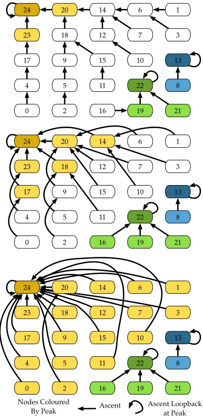
Figure 3: Monotone Path Construction. 3 iterations are required.
Since the trees form the connected components of the forest, we use pointer-doubling as described by Jaja [13] to collect the trees, as shown in Figure 3. In each iteration, each vertex points to its ascending neighbour’s neighbour, terminating at the peak. At the end of this process, every vertex has been assigned to a peak, as shown by the coloured groups: the colour attests to the existence of a monotone path from the vertex to the peak.
[image:5.612.77.277.515.660.2]la-Nodes Coloured By Peak
Edges Coloured By Peak
Saddle Candidates in Bold 24
22
21
15 10 13
0
8 1
20 14 6
23 18 12 7 3
17 9
4 5 11
[image:6.612.319.556.53.161.2]2 16 19
Figure 4: Saddle Candidate Identification. Edges are assigned to the same peak as their upper end. Any vertex whose edges lead to multiple peaks is a saddle candidate.
belled withp. If not, thenvis labelled withq, and a monotone path fromvtoqexists - and this implies the existence of a saddle be-tweenpandqthat is higher thans. This contradicts the assumption thatsis the governing saddle ofp, and the result follows.
We are therefore guaranteed that there is at least one edge from the governing saddleswhose upper end is already labelled withp. Except for other similar edges that lead fromstop, all edges whose upper ends lead to pmust have lower ends belows, and we can therefore identify the governing saddle by taking all of the edges in the mesh, grouping them into equivalence classes according to the peak which labels their upper end, and sorting by the lower end to find an edge that identifies the governing saddle.
This, however, assumes that we are examining only edges from saddles, which is harder to test than it may appear. We therefore define asaddle candidateto be a vertex which has ascending edges whose upper ends are labelled with at least two peaks: i.e. vertices in Figure 4 with ascending edges in two different colours. Every saddle is guaranteed to be a saddle candidate, but not vice versa: for example, vertex 5 is not a saddle, but is a saddle candidate.
However, for each peak, the governing saddle is thehighest sad-dle candidate with a monotone path to that peak. Suppose not. Then there is a saddle candidatecabove the governing saddles: all edges ascending fromcmust lead to p. Otherwise, eithercis a saddle higher than the governing saddle, or none of the edges lead to p, in which case, because if not,chas no monotone path to the peak, which is a contradiction. Either way, the result follows.
What this means is that we can choose all edges whose lower end is a saddle candidate, and sort them by the label of their upper end to group them into equivalence classes by the peak they lead to. We then sort again by the value of the lower end to identify the highest saddle candidate from which a path leads to the peak.
In practice, we take all edges in the mesh and sort them, using saddle candidacy as the primary sort, the ID of the peak as the sec-ondary index, and the value of the saddle as the tertiary index, as illustrated in Figure 5. This can be done either with a single sort using a comparator, or by a sequence of stable sorts.
The result of this sort is that all edges leading to each peakpare clumped in the sort array, and the rightmost (highest) such edge is adjacent either to the end of the array or an edge leading to a dif-ferent saddle. Given that we have now found each peak by finding the edge from its governing saddles, we now savesto an array prunedTo, i.e. prunedTo[p] =s. This represents removing the en-tire peak down to the level of the governing saddle.
This test for peak-saddle pairs is fully parallelised over all edges: only the edge that satisfies the conditions is allowed to assign the saddlesto the peakp, precluding write conflicts.
From Saddle Candidate 1 1 1 1 1 1 1 1 1 1 1 1 1 1 1 1 1 1 1 1
Peak for Upper End 24 24 24 24 24 24 24 24 24 24 24 24 24 24 24 22 22 22 22 22
Lower End 15 11 10 10 8 7 7 7 5 5 5 3 3 2 2 15 11 11 11 10
From Saddle Candidate 1 1 1 1 1 1 1 1 0 0 0 0 0 0 0 0 0 0 0 0
Peak for Upper End 22 22 22 22 13 13 13 13 24 24 24 24 24 24 24 24 24 24 24 24
Lower End 8 8 5 2 10 8 7 3 23 20 18 18 18 17 14 12 12 12 12 9
From Saddle Candidate 0 0 0 0 0 0 0 0 0 0 0 0 0 0 0 0
Peak for Upper End 24 24 24 24 24 24 24 24 24 24 24 24 22 22 22 22
Lower End 9 9 9 9 6 6 4 4 1 1 0 0 21 19 19 16
Figure 5: Peak-Saddle Pairing. Edges from non-saddle candidates (grey) are ignored, as are edges whose left neighbour has the same peak. The three marked edges identify peak-saddle pairs.
24
22
21
15 10 13
0
8 1
20 14 6
23 18 12 7 3
17 9
4 5 11
2 16 19
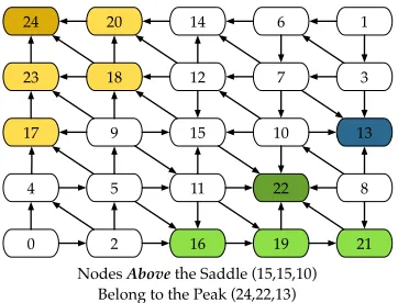
Nodes Above the Saddle (15,15,10)
[image:6.612.88.269.54.192.2]Belong to the Peak (24,22,13)
Figure 6: Assigning Regular Points. Regular points above the gov-erning saddle can only ascend to a single peak, and are assigned to it accordingly.
This process pairs critical points, but we must still process the regular points. In each iteration, once we have identified peak-saddle pairs, we exploit a simple property: any regular vertex above the governing saddlesof a peakpcan only have monotone paths top, and can therefore be assigned to that peak-saddle pair, shown inFigure 6 by assigning the maximum as a label.
Once peakpand its regular vertices are found, they are no longer needed, and the region is deleted [8]. However, monotone ascents to vertices inside this region are still needed, which is handled by redirecting any edge leading to a deleted vertex so that it instead ascends to the governing saddle, as shown in Figure 7.
Trunk Construction:In each pass, we prune all peaks to their governing saddles, flattening (or deleting them) to remove the re-gion above the governing. As a result, each governing saddle be-comes either a peak (e.g. 15 in our example) or a regular point (e.g. 10 in our example). We now recompute monotone paths and iterate: Figure 8 illustrates the next iteration for our example. Here, there is only one peak left at 15 and no saddles, so we have hit the base case and can assign all remaining vertices to the trunk which leads downwards from 15 to a virtual saddle at−∞.
Join Arc Connection:One final step remains: to compute the join arcs that connect all the vertices together so that we can com-pute the fully-augmented join tree. To do this, we observe that each vertex points to the next highest vertex in it’s peak-saddle join su-perarc, and construct this by sorting first on the vertex’ peak, then it’s value, as shown in Figure 9. Each vertex then points to it’s right-hand neighbour, unless this belongs to a different peak, in which case the vertex points to the saddle paired with the peak.
[image:6.612.350.531.214.352.2]22
21
15 10 13
0
8 1
20 14 6
23 18 12 7 3
17 9
4 5 11
2 16 19
24
[image:7.612.88.266.53.191.2]Edges to Pruned Nodes are Redirected to Saddle: Looped Edges are Deleted
Figure 7: Peak Pruning. Edges leading up to pruned vertices are truncated at the saddle’s isovalue, represented by redirecting them to the saddle. Pruned vertices and looped edges are removed.
15 10
0
8 1
14 6
12 7 3
9
4 5 11
2
After Final Iteration
Figure 8: Second Round of Monotone Path Construction. 15 is the last peak, and we transfer all vertices to the trunk of the tree.
To see this, consider Figure 10, which shows the join arcs we have just computed. We extracted peak-saddle pairs (24,15),(22,15),(13,10),(15,−∞): note that in the second pass, 10 was treated as a regular point, not a critical point. Once the indi-vidual join arcs have been constructed, however, the join superarcs can readily be broken up at these vertices.
3.2.2 Optimising Parallel Peak Pruning
We have just described an algorithm for constructing the join tree using only parallel operators. In practice, however, this algorithm is slow, as it carries regular vertices forward throughout the entire computation. We therefore optimise the algorithm by operating only on the critical points rather than the entire edge graph. As noted above, this can be done by defining a suitable join graph [6]. We further optimise by reducing the size of our arrays in each iter-ation, carrying forward only those vertices which are required.
Join Graph Construction:We start with the set of (local) joins and peaks, and add one edge to the join graph for each connected component of each join’s upper link. Since the vertex at the far end of this edge is not necessarily critical, we use the monotone paths from the previous phase to extend the edge to a peak. This gives us a valid join graph for our computation. This can be seen in Figure 11, where the grey vertices are carried forward. For example, vertex 15 is locally a saddle, so we extend the dotted edges to their cor-responding peak to get the initial chain graph shown in the second sub-figure. The rest of the algorithm then proceeds as described above, as shown in the rest of the figure.
Select Sorting Edges:In the above, we sortedalledges, rather than only edges ascending from saddle candidates. In order to
im-Peak 24 24 24 24 24 22 22 22 22 15 15 15 15 15 15 15 15 15 15 15 15 15 15 15 13 Vertex 24 23 20 18 17 22 21 19 16 15 14 12 11 10 9 8 7 6 5 4 3 2 1 0 13 Join Neighbour 23 20 18 17 15 21 19 16 15 14 12 11 10 9 8 7 6 5 4 3 2 1 0 -110
Figure 9: Join Arc Construction. Each vertex points to the next lowest in it’s peak-saddle superarc.
24
23 22
20 21
18 19
17 16
15
14
12
11 13
10
9
8
7
6
5
4
3
2
1
0
Figure 10: The Join Tree.
prove performance, we therefore add an extra phase that transfers only these ascending edges to a sorting array. As the algorithm pro-ceeds, this set naturally dwindles along with the vertices: we refer the reader to the next section for analysis.
Since this requires reduction operators, and the initial identifica-tion of the active graph means that all edges are used in the first pass, we place this at the bottom of the loop rather than the top.
Augmenting the Join Tree: By using a join graph as input, we compute the unaugmented join tree, but may still need an aug-mented join tree. We observe that our superarcs represent a branch decomposition of the join tree by vertex depth. In this, each peak is pruned to a saddle, which is in turn pruned to another saddle, until the trunk is reached - note that no peak can be pruned more times than the number of iterations through the main loop.
To augment with a regular vertexr, recall that we initially as-signedrto a peakpthrough monotone path construction. We prune rto a sequence of critical pointsc1=p,c2=prunedTo[c1], ...
un-til we find the firstcilower thanr, which attests thatrbelongs to
the superarc(ci−1,ci). We then compute join arcs as before. Since
each vertex operates independently, this too is parallelisable.
3.3 Parallel Combination of Merge Trees
As in the sweep and merge algorithm, we now wish to combine the two merge trees, and for this we need to ensure that the two trees share the same vertex set. We therefore augment each with the others nodes, and relabel all vertices and edges accordingly. Once we have done this, we batch transfers of edges from the merge trees to the contour tree in order to parallelise the combination phase.
Transfer Leaves: We observe that the transfer of a leaf from join or split tree in the sweep and merge algorithm is essentially a local operation. Here, as illustrated in Figure 12, we alternate transferring upper leaves from the join tree and lower leaves from the split tree. As we see in the first phase (Ia), we can transfer all upper leaves (grey) simultaneously. However, unlike the original sweep and merge, we do not delete these vertices immediately, as this causes write conflicts when updating edges. Instead, we flag the vertex as deleted, for later processing.
[image:7.612.88.265.248.373.2]up-Join Graph Edge
INITIAL JOIN GRAPH
24
22
15
10 13
REGULAR ASCENTS TO MAXIMA
24
22
21
15 10 13
0
8 1
20 14 6
23 18 12 7 3
17 9
4 5 11
2 16 19 Ascending Mesh Edge Monotone Path
FIRST PRUNING PASS
24
22
15
10 13
FIRST COLLAPSE
24
22
15
10 13
FINAL JOIN TREE
24
22
15
10 13
Join Tree Superarc / Pruning
[image:8.612.72.541.54.179.2]- ∞
Figure 11: Optimised Computation With Join Graph. (Left) We start with edges ascending from saddles (dotted) to their neighbours, then follow uphill to peaks, defining paths (dashed): eliminating duplicates gives us a valid join graph for merge tree computation. (Middle) In the first pass, edgen2n0andn1n0both ascend ton0, butn1is higher, and is therefore the governing saddle forn0. (Middle Right) We collapse
these peaks out of the graph, and redirectn2n0to point ton1instead, since we have prunedn0down to the level ofn1. (Right) Since we only
have one edge left, we have reached the base case and transfer−∞n2to the join tree, withn2treated as a regular point along−∞n2.
and down- degrees) leading downwards from an upper leaf to a crit-ical point, transfer their edges, and mark them as deleted.
Remove Deleted Vertices:Once the leaves and edges are trans-ferred to the contour tree (Phase Ia, grey), deleting them from the join tree is trivial, but deleting them from the split tree involves re-connecting edges. To do this, we use pointer-jumping once again, but only pointer-jump if our successor has been deleted. Thus, ver-tex 15 updates its successor to 17: even if there are multiple deleted vertices, the pointer-jumping will guarantee that we find the next valid node in logarithmic steps. This results in the join & split trees shown in Phase Ib, ready for the next phase.
Vertex Degree Update: We now update the active set of ver-tices and edges in both merge graphs ready for the next iteration, and recompute vertex up- and down- degrees by summing over all vertices, ready for the next pass.
3.4 Algorithmic Analysis
Consider the algorithmic cost of the optimised merge tree com-putation. In the initialisation stage, we take O(logE)steps and O(Elog(E)) work to initialise the array of edges, then a further O(logV)steps andO(VlogV)work to ascend to the maxima.
We then takeO(logE)more steps andO(ElogE)further work to find the topology graph to carry forward to the iteration. This graph will havet≤v<Vvertices andt<e<Eedges.
During the iterative stage, we haveO(logt)iterations, each of which involves a sort and several reductions withO(loge)steps and O(elog(e))work. Although the size of the tree diminishes in each iteration, there is a pathological case, so the most we can safely claim at present is that the iterative phase takes O(log(t)log(E) steps andO(Elog(t)log(E))work.
In the pathological case, exactly half of the vertices are critical (i.e. t=V/2), and there arer=V/2 regular points, all of which belong to the lowest (and final) superarc computed and have ascents to at least two maxima each. Here, while the numbertof critical points diminishes by half in each pass,rremains constant to the end, and each iteration therefore processesΘ(V)vertices and edges. Adding regular points takesO(logt)steps andO(Vlogt)work, then sort and reassignment inO(logV)steps andO(VlogV)work. For a regular mesh, initialisation can be done inO(E/V)steps andO(E)work, since the degree of each vertex isδ=O(E/V). Obviously, ifδ >logV, it may still be cheaper to use the more general algorithm, but 2d & 3d regular meshes have low degrees, so for large problem sizes, the reduction should be avoided.
In the iterative stage, the fact that we have a regular mesh works to our advantage again, as we can look at the connectivity of the upper link of each vertex to eliminate all regular points. However,
if we have a large number of vertices that are Morse critical but not connectivity critical, the same pathological case may occur. In practice, however, the collapse is significantly faster because we carry many fewer vertices forward between iterations.
In all, the computation therefore is limited by the iterative phase withO(logtlogE)steps andO(ElogtlogE)work, largely due to sorting. We note that it is possible to run a simplified version of the algorithm by retaining allV vertices andE edges throughout, with the same formal bound, but our early experience is that this is several orders of magnitude slower than the sweep and merge algorithm in serial, and twice as slow even for the version running on a Tesla K40 card. The optimisation to work with a diminishing graph size is therefore crucial in practice to keep runtimes down.
3.5 Contour Trees
For the final contour tree construction, the key question is how many iterations are needed to collapse the contour tree. We start by observing that the paired passes that remove upper and lower leaves between them remove all leaves. In order to forcelogt iterations, we would need to guarantee that no degree 2 vertices were left in the tree after each pass. Although many of them will be removed by the collapse described above, there is a pathological case.
In the pathological case, shown in Figure 12, a row of alternat-ing up and down edges (4−8−5−9−3−7−6) in the tree forms a repeatedW-motif. Here, when the upper and lower leaves are removed, only the endmost edges may be removed, causing the al-gorithm to serialise along theW. As a result, the best formal guar-antee for the algorithm is the graph diameter but, we usually take less than a logarithmic number of iterations.
Inside each iteration, the leaf transfer is fully parallel, taking O(1)steps andO(t) work in each pass. Collapsing regular and deleted vertices is logarithmic in nature, takingO(logt)steps and O(tlogt)work, as is the compression of the active graph and the recomputation of vertex degrees.
Thus, the formal cost of the merge phase, like the join and split tree computations, isO(log(t))steps andO(tlog2(t)work.
4 RESULTS
19 17 15 20 11 13 18 16 14 12 10 4 2 9 1 7 3 5 8 6 19 17 15 20 11 13 18 16 14 12 10 4 2 9 1 7 3 5 8 6
Contour Tree: Join Tree: Split Tree:
19 17 15 20 11 13 18 16 14 12 10 4 2 9 1 7 3 5 8 6 19 17 15 20 11 13 18 16 14 12 10 4 2 9 1 7 3 5 8 6 17 15 11 13 4 2 9 1 7 3 5 8 6
Contour Tree: Join Tree: Split Tree:
17 15 11 13 4 2 9 1 7 3 5 8 6 19 17 15 20 11 13 18 16 14 12 10 4 2 9 1 7 3 5 8 6
Contour Tree: Join Tree:
1 4 2 9 7 3 5 8 6 Split Tree: 19 17 15 20 11 13 18 16 14 12 10 4 2 9 1 7 3 5 8 6
Contour Tree: Join Tree:
9 7 3 5 8 9 7 3 5 8 Split Tree: 4 2 9 1 7 3 5 8 6 19 17 15 20 11 13 18 16 14 12 10 4 2 9 1 7 3 5 8 6
Contour Tree: Join Tree:
9 3 5 9 3 5 Split Tree: PHASE Ia: TRANSFER ALL UPPER LEAVES
PHASE Ib: COLLAPSE UPPER LEAF CHAINS
PHASE II: TRANSFER ALL LOWER LEAVES (NO LEAF CHAINS)
PHASE III: TRANSFER ALL UPPER LEAVES (NO LEAF CHAINS)
[image:9.612.114.501.56.542.2]PHASE IV: TRANSFER ALL LOWER LEAVES (NO LEAF CHAINS)
Figure 12: Parallelisation of Contour Tree Merge Phase. We first identify all upper leaves in parallel (top) and transfer them to the contour tree. After deleting these vertices from the join and split trees, we collapse regular chains from upper leaves (second), then repeat with lower and upper leaves, omitting collapses if there are no chains available. Note how the algorithm serialises along the W shape of vertices 8-5-9-3-7.
architectures, including GPUs (with Thrust’s CUDA backend) and multi-core CPUs (with Thrust’s OpenMP backend).
The performance and accuracy of the parallel peak pruning al-gorithm was evaluated using the GTOPO30 database, which con-tains elevation maps for the Earth at a horizontal grid spacing of 30 arc seconds (roughly one-half to one kilometer). The data consists of 33 tiles (excluding the special case of Antarctica), each 6000 x 4800 (28.8 million points). The full data set is 21,600 x 43,200, about 933 million points.
Verification was performed by comparing to the original sweep
and merge algorithm. All superarcs were output to file, sorted lex-icographically, and compared using the Linux diff utility. Verifica-tion was performed for each tile using each version of our algorithm (serial, Thrust OpenMP, and Thrust CUDA), as well as for the full data set using each version of our algorithm except Thrust CUDA (since the GPU memory was insufficient to run the full data set).
fastest of the five runs recorded for each variant on each tile. These tests were run on a 32-core 2.10GHz Intel Xeon E5-2683 v4 Broad-well CPU (two sockets with 16 cores each, and two threads per core), with 128 GB of RAM, and an Nvidia Tesla K40m with 2880 745 MHz CUDA cores and 12 GB of memory. The graph compares the implementations on the fastest tile and the slowest tile, as well as the average over all 33 tiles. The serial version of parallel pruning averaged about 40% slower than sweep and merge, but its primary advantage is its ability to run efficiently in parallel. For the mean over all tiles, the Thrust OpenMP version of parallel pruning had a speed-up of 13.1x relative to the serial version, and 9.2x relative to the original sweep and merge algorithm. We also implemented and tested a native OpenMP version of parallel pruning (not using Thrust), which was slightly slower than the Thrust OpenMP version (mean of 2.05 seconds compared to 1.25 seconds), indicating that the portability of Thrust did not negatively impact our performance. The Thrust CUDA version running on the GPU was faster still, with speed-ups of 21.0x and 14.8x relative to the serial parallel pruning version and to the sweep and merge version, respectively. GPU memory usage (obtained using cudaMemGetInfo) ranged between 2.6 GB and 3.8 GB for each tile, with the mean 3.1 GB.
▼✁✂✄☎ ▼☎ ✆ ✁✂✄☎ ▼ ✆✝✂✄☎ ❈✞✟✠ ✞✡☛☞☛rr☞ ✌✍✌✟✎✏✑✞☛♦☞❖✒ ❖✓ ✔☞ ✌✕r ✏
❚
✖
✗
✘
✙
✚
✘
✛
✜
✢
✣
✚
✤
✵
✶
✵
✷
✵
✸
✵
✹
✵
✻ ✥ ✦✧ ★✩✥✪ ✪
✩✥✻ ✫ ✩✥ ✦✻
★★✥✬ ✬ ★✻✥ ✫✬
★✥ ✦✬ ✩✥✭✧
✫✬✥✬✬ ✫✬✥✩✬
✫ ✥ ✦✪ ✦✥✮✩ ❙✯✰✐ ✱✲❙ ✳✯✯❡✱✴✺✼ ✯✰✽✯
❙✯✰✐ ✱✲✾✯✱✿✾✰✉✴✐ ✴✽
❀ ❁✰✉❂❃❄❡ ✯✴✼✾✾✯✱✿✾✰✉✴✐✴✽
[image:10.612.330.534.151.348.2]❀ ❁✰✉❂❃❅❆❇❉✾✯✱✿✾✰✉✴✐ ✴✽
[image:10.612.62.272.294.493.2]Figure 13: Comparison of join tree computation with the serial sweep and merge, serial version of parallel pruning, Thrust version of parallel pruning using the OpenMP backend on the CPU, and Thrust version of parallel pruning using the CUDA backend on the GPU. Results are shown for the fastest, slowest, and mean of the 33 GTOPO30 tiles.
Figure 14 shows the scaling of Thrust parallel pruning with the number of OpenMP threads. With four threads, the speed-up is 2.9x (parallel efficiency of 74%), and with eight threads the speed-up is 4.7x (parallel efficiency 58%). Beyond that, the speed-speed-up plateaus. Profiling using the VTune Performance Analyzer, with one GTOPO30 tile as the input, reports an overall memory bound metric of 43.4%, with the tree compression step and the monotone path construction reporting memory-bound metrics above 70%. VTune also identified the Thrust OpenMP stable sort as the largest potential gain, since it underutilises the available threads. The sta-ble sort gets called for a sort that uses a custom comparator, which we do when computing augmented arcs in the merge tree compu-tation and when finding the governing saddles in the chain graph.
Therefore, there may be an opportunity to further improve scala-bility by either optimizing the OpenMP stable sort or by adapting our algorithm to be able to avoid using it in favor of an unstable sort. The 21.0x speed-up of the GPU version relative to the serial version, running on cores with clock rate that is 2.8 slower than the GPU, indicates that the algorithm is able to achieve over 50x parallel speed-up.
0.5
1.0
2.0
5.0
10.0
Contour Tree Computation Scaling with OpenMP Threads
Number of OpenMP threads (log scale)
Time in seconds (log scale)
4 8 12 16 20 28
1
10.63
3.61
2.28 1.82
1.541.45 1.331.281.34
Figure 14: Scaling of the Thrust version of the parallel pruning algorithm with the number of OpenMP threads on a 32-core CPU. The ideal scaling line is shown in red.
Join Tree Contour Tree
Join and Contour Tree Timings for Full GTOPO30 Data
Time (seconds)
0
500
1000
1500
2000
2500
3000
346 321
30
2685
786
103
Serial Sweep and Merge Serial Peak Pruning Thrust OpenMP Peak Pruning
Figure 15: Comparison of serial sweep and merge, serial version of parallel pruning, and Thrust version of parallel pruning using the OpenMP backend running on the full 933 million point GTOPO30 data set. Timings are shown for the join and contour trees.
[image:10.612.332.528.428.615.2]billion points. The memory requirements precluded running this test on the GPU, but the other versions were run using a machine with 1.5 TB of memory and a 32-core 2.60GHz Intel Xeon E5-4650L Sandy Bridge CPU (four sockets with eight cores each, and two threads per core). In this case, the serial implementation of the parallel pruning algorithm was 3.1x faster than the original sweep and merge algorithm. Running with OpenMP, there was an addi-tional 8.6x speed-up, or 26.4x relative to sweep and merge. Tim-ings are also shown for computing only the join tree, which can also be useful independent of the full contour tree.
We note that internal representation of the contour tree can vary greatly between implementations, so timing and memory footprints should be compared only with a large margin for error.
5 CONCLUSIONS ANDFUTUREWORK
We have described the first pure data-parallel algorithm for the merge tree and contour tree in either unaugmented (canonical) or augmented form, with strong guarantees on computation time, and practical performance faster than the sweep and merge algorithm, with parallel speedup of at least one order of magnitude on GPU.
We intend to continue this line of research by implementing the algorithm for arbitrary meshes and graphs as well as 3d data, by ex-tending the scalability with a hybrid distributed/ data-parallel stage, and by adding geometric computation and simplification to allow the contour tree to be used forin situanalysis.
ACKNOWLEDGEMENTS
We would like to acknowledge EPSRC Grant EP/J013072/1 and the University of Leeds for supporting the first author’s study leave at Los Alamos National Laboratory. This work was supported by the U.S. Department of Energy, Office of Science, Office of Advanced Scientific Computing Research, of the U.S. Department of Energy under Contract No. DE-AC02-05CH11231 to the Lawrence Berke-ley National Laboratory (“Towards Exascale: High Performance Visualization and Analytics Program”) and under Award Number 14-017566 at Los Alamos National Laboratory (“XVis: Visual-ization for the Extreme-Scale Scientific-Computation Ecosystem”), with Lucy Nowell the program manager for both awards. We thank Li-ta Lo and Patricia Fasel for their contributions.
REFERENCES
[1] A. Acharya and V. Natarajan. A parallel and memory efficient algo-rithm for constructing the contour tree. InProceedings of the 2015 IEEE Pacific Visualization Symposium (PacificVis), pages 271–278, Apr. 2015.
[2] T. F. Banchoff. Critical Points and Curvature for Embedded Polyhe-dra.Journal of Differential Geometry, 1:245–256, 1967.
[3] G. Blelloch.Vector Models for Data-Parallel Computing. PhD thesis, MIT, 1990.
[4] H. Carr and D. Duke. Joint Contour Nets. IEEE Transactions on Visualization and Computer Graphics, 20(8):1100–1113, 2014. [5] H. Carr, C. Sewell, L.-T. Lo, and J. Ahrens. Hybrid data-parallel
contour tree computation. Technical Report LA-UR-15-24579, Los Alamos National Laboratory, 2015.
[6] H. Carr and J. Snoeyink. Representing Interpolant Topology for Con-tour Tree Computation. In H.-C. Hege, K. Polthier, and G. Scheuer-mann, editors,Topology-Based Methods in Visualization II, Mathe-matics and Visualization, pages 59–74. Springer, 2009.
[7] H. Carr, J. Snoeyink, and U. Axen. Computing Contour Trees in All Dimensions.Computational Geometry: Theory and Applications, 24(2):75–94, 2003.
[8] H. Carr, J. Snoeyink, and M. van de Panne. Flexible Isosurfaces: Simplifying and Displaying Scalar Topology Using the Contour Tree. Computational Geometry: Theory and Applications, 43(1):42–58, 2010.
[9] Y.-J. Chiang, T. Lenz, X. Lu, and G. Rote. Simple and Opti-mal Output-Sensitive Construction of Contour Trees Using Monotone
Paths. Computational Geometry: Theory and Applications, 30:165– 195, 2005.
[10] H. Edelsbrunner, J. Harer, and A. K. Patel. Reeb Spaces of Piecewise Linear Mappings. InProceedings of ACM Symposium on Computa-tional Geometry, pages 242–250., 2008.
[11] K. Heitmann, N. Frontiere, C. Sewell, S. Habib, A. Pope, H. Finkel, S. Rizzi, J. Insley, and S. Bhattacharya. The Q Continuum Simula-tion: Harnessing the Power of GPU Accelerated Supercomputers. To appear in the Astrophysical Journal Supplement., 2015.
[12] M. Hilaga, Y. Shinagawa, T. Kohmura, and T. L. Kunii. Topology Matching for Fully Automatic Similarity Estimation of 3D Shapes. ACM Transactions on Graphics, pages 203–212, 2001.
[13] J. JaJa. An Introduction to Parallel Algorithms. Addison-Wesley, 1992.
[14] A. G. Landge, V. Pascucci, A. Gyulassy, J. C. Bennett, H. Kolla, J. Chen, and P. T. Bremer. In-situ feature extraction of large scale combustion simulations using segmented merge trees. InSC14: Inter-national Conference for High Performance Computing, Networking, Storage and Analysis, pages 1020–1031, Nov. 2014.
[15] L.-T. Lo, C. Sewell, and J. Ahrens. PISTON: A Portable Cross-Platform Framework for Data-Parallel Visualization Operators. In Proceedings of Eurographics Symposium on Parallel Graphics and Visualization, pages 11–20, 2012.
[16] S. Maadasamy, H. Doraiswamy, and V. Natarajan. A hybrid parallel algorithm for computing and tracking level set topology. InHigh Per-formance Computing (HiPC), 2012 19th International Conference on, pages 1–10. IEEE, Dec. 2012.
[17] D. Morozov and G. Weber. Distributed Merge Trees.ACM SIGPLAN Notices, 48(8):93–102, 2013.
[18] D. Morozov and G. Weber. Distributed Contour Trees. In P.-T. Bre-mer, I. Hotz, V. Pascucci, and R. Peikert, editors,Topological Methods in Data Analysis and Visualization III, Mathematics and Visualization, pages 89–102. Springer, 2014.
[19] V. Pascucci and K. Cole-McLaughlin. Parallel Computation of the Topology of Level Sets.Algorithmica, 38(2):249–268, 2003. [20] V. Pascucci, K. Cole-McLaughlin, and G. Scorzelli. The
TOPOR-RERY: Computation and Presentation of Multi-Resolution Topology, pages 19–40. Springer-Verlag, Berlin Heidelberg, Germany, 2009. Preliminary version appeared in the proceedings of the IASTED con-ference on Visualization, Imaging, and Image Processing (VIIP 2004), 2004, pp.452-290.
[21] G. Reeb. Sur les points singuliers d’une forme de Pfaff compl`etement int´egrable ou d’une fonction num´erique. Comptes Rendus de l’Acad`emie des Sciences de Paris, 222:847–849, 1946.
[22] C. Sewell, K. Heitmann, L.-T. Lo, S. Habib, and J. Ahrens. Utilizing Many-Core Accelerators for Halo and Center Finding within a Cos-mology Simulation. In submission., 2015.
[23] C. Sewell, L.-T. Lo, and J. Ahrens. Portable Data-Parallel Visual-ization and Analysis in Distributed Memory Environments. In Pro-ceedings of the IEEE Symposium on Large-Scale Data Analysis and Visualization (LDAV), pages 25–33, 2013.
[24] S. Takahashi, T. Ikeda, Y. Shinagawa, T. L. Kunii, and M. Ueda. Algo-rithms for Extracting Correct Critical Points and Constructing Topo-logical Graphs from Discrete Geographical Elevation Data.Computer Graphics Forum, 14(3):C–181–C–192, 1995.
[25] R. E. Tarjan. Efficiency of a good but not linear set union algorithm. Journal of the ACM, 22:215–225, 1975.
[26] M. van Kreveld, R. van Oostrum, C. L. Bajaj, V. Pascucci, and D. R. Schikore. Contour Trees and Small Seed Sets for Isosurface Traversal. InProceedings, 13th ACM Symposium on Computational Geometry, pages 212–220, 1997.
[27] M. J. van Kreveld, R. van Oostrum, C. L. Bajaj, V. Pascucci, and D. R. Schikore. Topological Data Structures for Surfaces: An Introduction for Geographical Information Science, chapter 5: Efficient contour tree and minimum seed set construction, pages 71–86. John Wiley & Sons, May 2004.