Exploring sampling in the detection of multicategory EEG signals

Research Article

Exploring Sampling in the Detection of

Multicategory EEG Signals

Siuly Siuly,

Enamul Kabir,

Hua Wang,

and Yanchun Zhang

1_{Centre for Applied Informatics, College of Engineering and Science, Victoria University, P.O. Box 14428,}

Melbourne, VIC 8001, Australia

2_{School of Agricultural, Computational and Environmental Sciences, University of Southern Queensland,} Toowoomba, QLD 4350, Australia

3_{School of Computer Science, Fudan University, Shanghai 200433, China}

Correspondence should be addressed to Siuly Siuly; siuly [email protected]

Received 24 February 2015; Accepted 30 March 2015

Academic Editor: Po-Hsiang Tsui

Copyright © 2015 Siuly Siuly et al. This is an open access article distributed under the Creative Commons Attribution License, which permits unrestricted use, distribution, and reproduction in any medium, provided the original work is properly cited.

The paper presents a structure based on samplings and machine leaning techniques for the detection of multicategory EEG signals where random sampling (RS) and optimal allocation sampling (OS) are explored. In the proposed framework, before using the RS and OS scheme, the entire EEG signals of each class are partitioned into several groups based on a particular time period. The RS and OS schemes are used in order to have representative observations from each group of each category of EEG data. Then all of the selected samples by the RS from the groups of each category are combined in a one set named RS set. In the similar way, for the OS scheme, an OS set is obtained. Then eleven statistical features are extracted from the RS and OS set, separately. Finally this study employs three well-known classifiers:k-nearest neighbor (k-NN), multinomial logistic regression with a ridge estimator (MLR), and support vector machine (SVM) to evaluate the performance for the RS and OS feature set. The experimental outcomes demonstrate that the RS scheme well represents the EEG signals and thek-NN with the RS is the optimum choice for detection of multicategory EEG signals.

1. Introduction

Efficiently detecting multicategory EEG signals is benefi-cial for handling neurological abnormalities and also for evaluating the physiological state of the brain for a broad range of applications in biomedical community. EEG signals indicate the electrical activity of the brain and contain useful information about the brain state to study brain function [1]. The identification of different categories EEG signals is traditionally performed by experts based on the visual interpretation. The manual scoring is subject to human errors and it is time consuming, costly process and not sufficient

enough for reliable information [2, 3]. Thus there is an

ever-increasing need for developing automatic systems to evaluate and diagnose multicategory EEG signals to prevent the possibility of the analyst missing information. Complex characteristics of EEG signals (e.g., poor signal-to-noise ratio,

nonstationary, and aperiodic) require employment of robust detection algorithms in order to achieve reasonable detection performance. Hence, designing efficient detection algorithms has been an important goal and highly attractive area to ensure a proper evaluation and treatment of neurological diseases for this study.

In order to perform the detection of signal’s category, first the most important task is to extract distinguishing features or characteristics from EEG data that can describe the morphologies or the key properties of the signals. The features significantly affect the accuracy of detecting EEG signals [4]. The features characterizing the original EEG are used as the input of a classifier to differentiate different categories of EEGs. As optimal features play a very important role in the performance of a classifier, this study intends to find out a robust feature extraction process for the detection of multicategory EEG signals.

Recently, various approaches for automatic detection of multicategory EEG signals have been reported. Siuly and Li [5] proposed a statistical framework for multiclass EEG signal classifications. They developed an optimum allocation scheme based on the variability of observation within a group (based on specific time) of the EEG data and selected a rep-resentative sample. The reprep-resentatives were fed to the least square support vector machine (LS-SVM) classifier instead of taking representative features that may be a limit for further consideration of a detection technique. An approach based on a cascade of wavelet-approximate entropy was introduced by Shen et al. [6] for the feature extraction in the EEG signal clas-sification. They tested three existing methods, support vector

machine (SVM), 𝑘-nearest neighbour (𝑘-NN), and radial

basis function neural network (RBFNN), and determined the classifier of best performance. Acharjee and Shahnaz [7] had a study on twelve Cohen class kernel functions to transform EEG data in order to facilitate the time frequency analysis. The transformed data formulated a feature vector consisting of modular energy and modular entropy, and the feature vector was fed to an artificial neural network (ANN) classifier. Muthanantha Murugavel et al. [8] had conducted a study based on Lyapunov feature and a multiclass SVM for the

detection of EEG signals. ¨Ubeyli [9] presented an approach

that integrated automatic diagnostic systems with spectral analysis techniques for EEG signal classification. The wavelet coefficients and power spectral density (PSD) values obtained by eigenvector methods were used as features, and these features were fed to each of the seven classification algorithms (SVM, recurrent neural networks (RNN), PNN, mixture of experts (ME), modified mixture of experts (MME), com-bined neural networks (CNN), and multilayer perceptron

neural network (MLPNN)). ¨Ubeyli [10] provided another

algorithm based on eigenvector methods and multiclass SVMs with the ECOC for the classification of EEG signals. In the feature extraction stage, three eigenvector methods such as the Pisarenko, MUSIC, and minimum norm were used to obtain the PSD values of the EEG signals that were employed as the input of the multiclass SVMs. For the detection of multiclass EEG signals, Guler and Ubeyli [11] had examined again SVM, PNN and MLPNN on wavelet coefficients and lyapunov exponents features. The experimental outcomes of that research demonstrated that the SVM classifier performed better than the other two classifiers with these features.

In the literatures, the majority of the existing methods cannot appropriately handle a large amount of EEG data due to their structure. On the other hand, most of the methods

were limited in their success and effectiveness [10, 11]. In

addition, some of the existing methods of the feature extrac-tion stage are not the right choice for getting representative features from the original EEG data due to its nonstationary and aperiodic characteristic (e.g., Fourier transformation) [12]. Although numerous methods have been developed for feature extraction stage, little attention has been paid in the using of sampling, which is a fundamental component in statistics to represent information from original entire EEG signals. Sampling is very effective if the population (a group of observations) is heterogeneous and is very large in size. An effective sample (a subset of the group of observations)

of a population represents an appropriate extraction of the useful data which provides meaningful knowledge of the important aspects of the population. It will be more expedient if the population is divided into several groups according to a specific characteristic and then selects representative samples from each and every subgroup depending on group size such that the entire samples reflect the whole population. As EEG recordings normally include a vast amount of data and the data is generally heterogeneous with respect to time period, it is a natural expectation that dividing the whole EEG recordings into some subgroups with respect to time and then taking representative samples from each subgroup would improve the performance of a classifier. This improvement is achieved in this paper for classifying the multicategory EEG signals.

Challenging these issues, this paper explores the idea of the sampling for getting representative information out from raw EEG data for the detection of multicategory EEG signals. In this study, we develop a structure for the detection of multicategory based on sampling for the feature extraction stage proposing two schemes: random sampling (RS), optimum allocation sampling (OS). This study uses the RS and OS schemes to evaluate how efficient they are to select representative samples from each segment of each category of

EEG data discussed in detail inSection 2.1. “Representative

sample” means a sample that is selected randomly from a segment (a short time window) called “population” and each observation of the population has a known, nonzero chance of being selected in the sample. In the proposed approach, firstly we segment the whole EEG signals of a class (a category) into several groups according to a particular time period. Then we draw samples from each group of a class using the RS and OS technique, separately. After that, for each of the RS and OS schemes, we make two separate sample sets called “RS” set and “OS” set combining all of their samples from each group of that class (detailed discussion

in Section 2.1). After that we extract descriptive features

from the RS set and the OS set of that class (discussed in Section 2.2). The same procedure applies for all of the classes of EEG data. The accumulation of all features from all of the classes constitutes a feature vector for the RS scheme and also for the OS scheme. The collection of all features from all class of EEG signals for the RS and OS scheme is employed as an input set in the classifier.

To achieve a higher detection performance, the set of input features and the choice of the machine learning techniques are crucial. If a feature provides large interclass differences for different classes, the technique can exhibit a better performance. In order to find out an effective model with highest accuracy for detection of multicategory EEG signals, in this paper we test three machine learning

tech-niques, namely,𝑘-nearest neighbours (𝑘-NN), multinomial

Selecting optimum value for parameters

Cross validation Features

Estimated class labels Detection

model Training set

Testing set

Features EEG

signals of a class

Seg₁

Seg₂

Seg_k ...

RS

OS

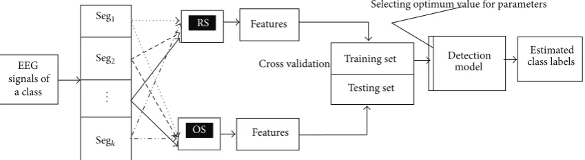
Figure 1: Structure of the proposed method for the detection of multicategory EEG signals.

are repeated for 20 times with the reported three classifiers to observe the consistency of the structure. We also compare our proposed algorithms with the other existing well-known algorithms in the literature. The experimental results show that the proposed RS based algorithm can detect perfectly for each class of EEG signals in terms of all possible detection

parameters by using the𝑘-NN classifier.

The rest of the paper is organized as follows.Section 2

presents a description of the proposed methodology in detail. In this section, we also briefly describe the three classifiers and the features extraction methods used in this paper. The description of benchmark EEG data and experimental

design are provided inSection 3. InSection 4, we present the

experimental results of the three classifiers with a detailed discussion. This section also provides a comparative report in the context of existing studies in the literature. Finally,

concluding remarks are included inSection 5.

2. Method

The detection technique that is developed in this study is

comprised of three key structures.The first oneis to select

representative samples from each and every segment of an entire signal data of a category (e.g., healthy subject with eye open; epileptic patient during seizure activity). In order to select a representative sample, we employ random sampling (RS) and optimum allocation sampling (OS) scheme, sepa-rately to compare their effectiveness. Then we select samples by using the RS and OS techniques from each segment of a class and consequently make two different groups (“RS” and

“OS”) as shown inFigure 1. The subsequentsecond oneis to

extract representative features from each of the RS and OS groups to represent the distribution of data pattern and then to integrate all of the features of each class in a matrix that is

called feature vector set.The third oneis the use of detection

method, which is based on the machine learning algorithms.

We herewith employ three different classifiers:𝑘-NN, MLR,

and SVM for the detection of multicategory EEG signals. Integration of the second and third structure results into a novel time series detection technique. We use this integrated technique to identify multicategories EEG signals.

2.1. Sampling. In statistics, sampling is a process of selection of a subset of individuals from a group of observations (called

Sampling

Population Sample

Figure 2: An example of a visual representation of the sampling process.

population) to represent the whole population. Figure 2

illustrates how observations are selected in a sample from

population. As shown in Figure 2, the population of size

12 consists of three colour observations such as red, green, and gray, where there are three elements of green colour, six elements of red colour, and three elements of gray colour. In the sample, two red, one green, and one gray colour elements are selected from the population through a random sampling process. Thus only four elements are selected in the sample that represents the whole population of size 12. In the proposed framework, before using sampling, we segment the EEG signals of each class into several groups based on a particular time period in order to have representative values of a specific time period.

The reason of segmentation is to properly account for possible stationarities assignal processing methods requiring stationarity of signals while EEG signals are nonstationary and aperiodic and the magnitudes of the signals are changed over time. In order to have representative values of a specific time period, the EEG signals of a class are divided into

some mutually exclusive groups. As can be seen inFigure 1,

this study partitions the EEG signals of each class into

𝑘nonoverlapping segments denoted by Seg₁,Seg₂, . . . ,Seg_𝑘

considering a particular time period. Then, the representative observations are selected from each segment by the RS and OS technique, separately. Depending on the selection process, the algorithm consists of two types, provided below.

data of a class (called population) is determined by using(1)

and(2)[13–16]:

SS= 𝑧

2_{× 𝑝 × (1 − 𝑝)}

𝑒2 , (1)

where SS means the sample size;𝑧 is the standard normal

variate (𝑍-value) for the desired confidence level; 𝑝is the

assumed proportion in the target population estimated to

have a particular characteristic; and𝑒is the margin of errors

or the desired level of precision. If population is finite, the required sample size for each class is given by

𝑛 = SS

1 + (SS− 1) /Popu, (2)

where Popu means population size and 𝑛 is the required

sample size. After determining the sizes, we select the rep-resentative samples directly from the respective segments of each class. Then all of the selected samples from the segments of each class are combined together in a set (called RS set) from where representative characteristics are obtained as

features discussed inSection 2.2.

2.1.2. Optimum Allocation Sampling (OS). In this scenario, we firstly determine the required sample size from the whole EEG signals with a desired confidence interval and confi-dence level. Then we determine the required sample from each segment using the optimum allocation (OS) scheme by

(3)that considers the variability among the signals in each

segment. A detailed description of the OS is available in

[5,14]:

𝑛 (𝑖) = 𝑁𝑖√∑

𝑝

𝑗=1𝑠𝑖𝑗2

∑𝑘_𝑖=1(𝑁_𝑖√∑𝑝_𝑗=1𝑠_𝑖𝑗2₎× 𝑚

𝑖 = 1, 2, . . . ., 𝑘; 𝑗 = 1, 2, . . . , 𝑝,

(3)

where𝑛(𝑖)is the required sample size of the𝑖th Seg;𝑁_𝑖is the

data size of the𝑖th Seg;𝑠_𝑖𝑗2is the variance of the𝑗th channel

of the𝑖th Seg; and𝑚is the sample size of the EEG recording

of a class obtained. Finally, we select the required sample from each segment based on the OS structure. Then all of the selected samples from the segments of each class are united in a set (named OS set) and representative characteristics are

extracted from the OS set as discussed inSection 2.2.

2.2. Feature Extraction. Feature extraction aims at describ-ing many data points into fewer parameters, which are termed “features” that represent important pattern of data distribution. The feature extraction process transforms the original signals into a feature vector. These features represent the behaviours of the EEG signals, which are particularly significant for recognition and diagnosing purposes. In this paper, the eleven statistical features from each segment of EEG channel data are extracted as the valuable parameters for the representation of the characteristics of the original

EEG signals which are mean (𝑋Mean), median (𝑋Me), mode

(𝑋Mo), standard deviation (𝑋SD), first quartile (𝑋Q1), third

quartile (𝑋_Q3), interquartile range (𝑋IQR), skewness (𝑋𝛽1),

kurtoses (𝑋_𝛽2), minimum (𝑋_Min), and maximum (𝑋_Max). It

is noted that these features are the most representative values to describe the original EEG signal in each segment. The

feature set is denoted by{𝑋Mean,𝑋Me,𝑋Mo,𝑋Q1,𝑋Q3,𝑋IQR,

𝑋SD,𝑋𝛽₁, 𝑋𝛽₂, 𝑋Min, 𝑋Max}. Out of above eleven features,

𝑋Min, 𝑋Max, 𝑋Me (also called 2nd quartile),𝑋Q1, and 𝑋Q3

are together called a five-number summary. A five-number summary is sufficient to represent a summary of a large dataset [17–19]. It is well known that a five-number summary from a database provides a clear representation about the characteristics of a dataset.

Again an EEG data can be symmetric or skewed. For a symmetric distribution, appropriate measures for measuring the centre and variability of the data are the mean and the standard deviation, respectively. For skewed distributions, the median and the interquartile range (IQR) are the appro-priate measures for measuring the centre and spread of the

data [17,19]. Mode is the value in the dataset that occurs most

often. The mode for a continuous probability distribution is defined as the peak of its histogram or density function.

Skewnessdescribes the shape of a distribution that charac-terizes the degree of asymmetry of a distribution around its

mean [17,19].kurtosisis a descriptor of the shape of a data

distribution whether the data are peaked or flat relative. It quantifies whether the shape of the data distribution matches the normal distribution. For these reasons, we consider these eleven statistical features as the valuable parameters for representing the characteristics of the EEG signals and also brain activity as a whole. The accumulations of all obtained features from all segments of all classes are employed as the input for the three different classifiers.

2.3. Detection. In this work, this study employs three

clas-sifiers: 𝑘-nearest neighbours (𝑘-NN), multinomial logistic

regression with ridge estimators (MLR), and support vector machine (SVM) to evaluate the performance for the RS and OS feature set. The reason of choosing of these classifiers for this study is its simplicity and effectiveness in implementa-tion. They is also very powerful and fastest learning algorithm that examines all its training input for classification in this area. The following sections provide a brief idea about the classification methods that are used in this research.

2.3.1. 𝑘-Nearest Neighbours (𝑘-NN). The 𝑘-NN is a very intuitive method in which the classifier labels observations based on their similarity between observations in the training data. Among the various methods of supervised statistical

pattern recognition, the 𝑘-NN rule achieves consistently

high performance, without a priori assumptions about the distributions from which the training examples are drawn

[20]. Given a query vector 𝑥₀ and a set of 𝑁 labelled

instances {𝑥_𝑖, 𝑦_𝑖}𝑁₁, the task of the classifier is to predict

the class label of𝑥₀ on the predefined𝑃classes. The𝑘-NN

classification algorithm tries to find the𝑘-nearest neighbors

of𝑥₀ and uses a majority vote to determine the class label

applies Euclidean distances as the distance metric [21]. An

appropriate value should be selected for𝑘, because the success

of classification is very much dependent on this value. There

are several methods to choose thek-value; one modest idea is

to run the algorithm many times with differentk-values (𝑘 =

1, 2, . . . , 20) and choose the one with the best performance. A

detailed discussion of this method is available in [22,23].

2.3.2. Multinomial Logistic Regression Classifier with a Ridge Estimator (MLR). The MLR have become increasingly popu-lar with the easy availability of appropriate computer routines. Ridge estimators are used in MLR to improve the param-eter estimates and to diminish the error made by further prediction when maximum likelihood estimators (MLE) are nonunique and infinite to fit data. When the number of explanatory variables is relatively large and or when the explanatory variables are highly correlated, the estimates of parameters are unstable, which means they are not uniquely defined (some are infinite) and/or the maximum of

log-likelihood is achieved at 0 [24, 25]. In this situation, ridge

estimators are used to generate finiteness and uniqueness of MLE to overcome such problems. Let the response variable

𝑌 ∈ {1, 2, . . . , 𝑘}have𝑘possible values (categories). If there

are𝑘classes for𝑛instances with𝑚attributes (explanatory

variables), the parameter matrix𝐵to be calculated will be

𝑚 × (𝑘 − 1). The probability for class𝑗with the exception of the last class is

𝑃_𝑗(𝑋_𝑖) = exp(𝑋𝑖𝐵𝑗)

(∑𝑘_𝑗=1exp(𝑋_𝑖𝐵_𝑗) + 1). (4)

The last class has the probability

1 −𝑘−1∑

𝑗=1𝑃𝑗(𝑋𝑖) =

1

∑𝐾−1_𝐽=1 exp(𝑋_𝑖𝐵_𝑗) + 1. (5)

The (negative) multinomial log-likelihood is thus

𝐿 = −∑𝑛

𝑖=1

{ { {

𝑘−1

∑

𝑗=1

(𝑌_𝑖𝑗×In(𝑃_𝑗(𝑋_𝑖))) + (1 − 𝑘−1

∑

𝑗=1

𝑌_𝑖𝑗)

×In(1 − 𝑘−1

∑

𝑗=1

𝑃_𝑗(𝑋_𝑖))}_} }

+ridge× 𝐵2.

(6)

In order to find the matrix 𝐵for which 𝐿is minimised, a

Quasi-Newton Method is used to search for the optimized

values of the𝑚 × (𝑘 − 1)variables [24]. Note that before we

use the optimization procedure, we “squeeze” the matrix𝐵

into𝑚 × (𝑘 − 1)vector. A detailed description of the MLR can

be found in [24,25].

2.3.3. Support Vector Machine (SVM). The SVM is most pop-ular machines learning tool that can classify data separated by nonlinear and linear boundaries, originated from Vapnik’s statistical learning theory [26]. The main concepts of the SVM are to first transform input data into a higher dimensional

space and then construct an optimal separating hyper plane (OSH) between the two classes in the transformed space

[27,28]. Those data vectors nearest to the constructed line

in the transformed space are called the support vectors that contain valuable information regarding the (OSH). SVM is an approximate implementation of the “method of structural risk minimization” aiming to attend low probability of gen-eralization error. In most real life problems (including our problem), the data are not linearly separable. In order to solve

nonlinear problems, SVMs use a kernel function [27, 28],

which allows better fitting of the hyperplane to more general datasets. In more recent times, SVMs have been extended to solve multiclass-classification problems. One frequently used method in practice is to use a set of pairwise classifiers, based on one-against-one decomposition [28]. The decision function for binary classification is as follows:

𝑓 (𝑥) =sgn( 𝑠

∑

𝑖=1

𝑦_𝑖𝛼_𝑖𝑘 (𝑥_𝑖, 𝑥) + 𝑏) ; 0 < 𝛼_𝑖< 𝐶, (7)

where sgn is the signum function,𝐾(𝑥_𝑖, 𝑥)is kernel function,

and𝑏is the bias of the training samples. In this paper, radial

basis function (RBF) kernel is considered as a choice for identifying different categories EEG signals because it was

found to give the best classification performance. Here𝐶is

regularization parameter used to tune the trade-off between minimizing empirical risks (e.g., training error) and the complexity of the machine is always set to its default value;

namely, 𝐶 = 𝑁/ ∑𝑁_𝑖=𝐾(𝑥_𝑖, 𝑥), where𝑁 is the size of the

training set.

In the multiclass classification, the SVMs work by using

a collection of decision functions𝑓_𝑘𝑙, and hereklindicates

each pair of classes selected from separated target classes. The class decision can be achieved by summing up the pairwise decision functions [28]

𝑓_𝑘(𝑥) =∑𝑛

𝑖=1

sgn(𝑓_𝑘𝑙(𝑥)) . (8)

Here 𝑛 is the number of separated target classes. The

algorithm proceeds as follows: assign a label to the class:

arg max𝑓_𝑘(𝑥), (𝑘 = 1, 2, . . . , 𝑛). The pairwise classification

converts then-class classification problem into𝑛(𝑛−1)/2

two-class problems which cover all pairs of two-classes. An overview of SVM pattern recognition techniques may be found in [26– 28].

3. Data and Experimental Design

0 5 10 15 20 25 0

200

0 5 10 15 20 25

0 500

0 5 10 15 20 25

0 500

0 5 10 15 20 25

0 200

0 5 10 15 20 25

0 2000

Time (s) Time (s)

Time (s) Time (s) Time (s) −200

−200 −500

−500

−2000

Am

p

li

tude

(

𝜇

V)

Am

p

li

tude

(

𝜇

V)

Am

p

li

tude

(

𝜇

V)

Am

p

li

tude

(

𝜇

V)

Am

p

li

tude

(

𝜇

V)

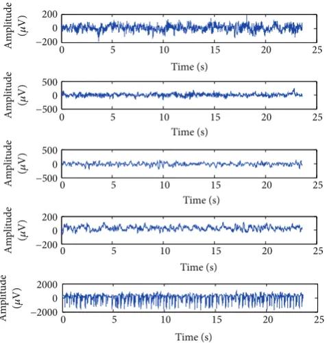
Figure 3: Exemplary EEG signals from each of the five sets. From top to bottom: class Z, class O, class N, class F, and class S.

scheme. Volunteers were relaxed in an awake state with eyes open (class Z) and eyes closed (class O), respectively. Sets C, D, and E (denoted classes N, F, and S, resp.) originated from presurgical diagnosis. Segments in Set D (class F) were recorded from within the epileptogenic zone and those in Set C (class N) from the hippocampal formation of the opposite hemisphere of the brain. While Set C (class N) and Set D (class F) contained only activity measured during seizure free intervals, Set E (class S) only contained seizure activity. All EEG signals were recorded with the same 128-channel amplifier system, using an average common reference. After 12-bit analog-to-digital conversion, the data were written continuously onto the disk of a data acquisition computer system at a sampling rate of 173.61 Hz. Band-pass filter settings were 0.53–40 Hz (12 dB/oct.). In this work, five classes’ (Z to S) classification problems, called multiclass classification, are performed from the above dataset in order to verify the performance of the proposed method. All the EEGs from the dataset are used and they are classified into five different classes: Z, O, N, F, and S, which can be denoted by Z-O-N-F-S. Exemplary EEGs of each of the five classes are

depicted inFigure 3.

3.2. Training and Testing: Cross Validation. There are many choices of how to divide the data into training and test sets [31]. In order to reduce the bias of training and test data,

we propose employingk-fold cross validation technique [31–

34] considering 𝑘 = 10 in this study. This technique is

implemented to create the training set and testing set for

evaluation. Generally, with k-fold cross validation, feature

vector set is divided into𝑘subsets of (approximately) equal

size. The proposed classifiers are trained and tested𝑘times,

in which one of the subsets from training is left out each time and tested on the omitted subset. Each time, one of the subsets

(folds) is used as a test set and the other𝑘−1subsets (folds) are

put together to form a training set. Then the average accuracy

across all𝑘trials is computed for consideration.

3.3. Select Optimum Values of the Parameters of the Classifiers.

As mentioned before, this study uses three classification

methods:𝑘-NN, MLR, and SVM. The𝑘-NN model has only

one parameter 𝑘 which refers to the number of nearest

neighbors. By varying 𝑘, the model can be made more or

less flexible. In this study, we select appropriate𝑘-value in

automatic process following𝑘selection error log as there is

no simple rule for selecting𝑘. We consider the range of𝑘

-value in between 1 and 30 and pick an appropriate𝑘-value that

results in lowest error rate as the lowest error rate refers to the best model. In the experimental results, we obtain the lowest

error rate for𝑘 = 1. In the MLR method, the parameters are

obtained automatically through a ridge estimator discussed

in Section 3.3. For the SVM, the RBF kernel function is

employed as an optimal kernel function over different kernel functions that were tested. As there are no specific guidelines to set the values of the parameters for the MLR and the SVM classifiers, we consider the parameter values that have been used in WEKA default parameters settings.

3.4. Performance Evaluation of Classification Schemes. Cri-teria for evaluating the performance of a classifier are an important part in its design. In this study, we assess the performance of the proposed classifiers through most of the criteria that are usually used in biomedical research such as true positive rate (TPR) or sensitivity, false alarm rate (FAR)

or false positive rate or 1−specificity, precision, recall, 𝐹

-measure, accuracy, kappa statistics, mean, receiver operating characteristic (ROC) curve area, and absolute error (MAE). These criteria allow estimating the behaviour of the classifiers on the extracted feature data. The evaluation measure most used in practice is accuracy rate which evaluates effectiveness of the classifier by its percentage of correct prediction [35– 37]. The TPR (sensitivity) provides the fraction of positive cases that are classified as positive and it is also called

recall [18, 31, 33, 38]. The FAR [5] is the percentage of

false positives predicted as positive from negative class. The FAR usually refers to the expectancy of the false positive ratio. Precision (positive predictive value) is a measure which estimated the probability that a positive prediction is correct.

𝐹-measure is a combined measure for precision and recall

calculated as 2 ∗ Precision ∗ Recall/(Precision + Recall).

0 10 20 30 40 50 60 70 80 90 100 0

50 100

Sample values

Am

p

li

tude

RS OS

Original EEG signal from class Z −200

−150 −100 −50

(a)

RS OS

0 10 20 30 40 50 60 70 80 90 100

0 500 1000

Sample values

Am

p

li

tude

−1500 −1000 −500

Original EEG signal from class S

(b)

Figure 4: (a) Exemplary pattern of the RS and OS data with their respective original EEG signal from class Z (healthy subject with eye open). (b) Exemplary pattern of the RS and OS data with their respective original EEG signal class S (epileptic patient during seizure activity).

4. Experimental Results and Discussions

To validate the effectiveness of the proposed approach, we examine this scheme on the epileptic EEG database. The analyses of the RS and OS application are presented in

Section 4.1. Section 4.2 reports the resultant classification

performance of the proposed method. This section also provides a comparison between the proposed method and four well-known existing methods. All of the calculations are carried out in MATLAB (version 7.14, R2012a). We

experimented three classification algorithms: 𝑘-NN, MLR

with a ridge estimator, and SVM implemented in WEKA machine learning toolkit [40]. LIBSVM (version 3.2) [41] is used for the SVM classification in WEKA.

4.1. Analysis on the Application of RS and OS. According

to our framework as shown inFigure 1, at first we segment

each of the five classes into four parts (𝑘 = 4). As every

channel of a class contains 4097 data points of 23.6 seconds,

in each class, the sizes of the four segments, Seg₁, Seg₂, Seg₃,

and Seg₄, are𝑁₁ = 1024,𝑁₂ = 1024,𝑁₃ = 1024, and 𝑁₄ =

1025, respectively, and each segment contains the data for 5.9 sec. Then we select a sample (a representative subset of a segment) from each of the four segments in every class using the RS and OS technique, separately as discussed in Section 2.1. The calculated required sample sizes under the

RS and OS technique are reported inTable 1. In the RS, the

sample sizes for each segment are calculated by(2)whereas

(3)is used to compute the sample sizes for each segment in

the OS scheme. Using the calculated sample sizes displayed in Table 1, the samples are selected from the respective segments of that class. It is important to note that the sample selection

procedure is repeatedtwentytimes in both the RS and OS

schemes to achieve most reliable and consistent results. To illustrate exemplary pattern of the RS and OS sample,

Figures4(a)and4(b)are presented for a segment of a class.

Figure 4(a) displays an exemplary pattern of the RS and

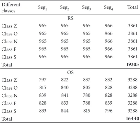
Table 1: Obtained sample sizes by the OS and RS technique from each segment of every class.

Different

classes Seg1 Seg2 Seg3 Seg4 Total RS

Class Z 965 965 965 966 3861

Class O 965 965 965 966 3861

Class N 965 965 965 966 3861

Class F 965 965 965 966 3861

Class S 965 965 965 966 3861

Total 19305

OS

Class Z 797 822 837 832 3288

Class O 815 840 805 828 3288

Class N 839 841 780 828 3288

Class F 828 833 788 839 3288

Class S 833 844 815 796 3288

Total 16440

OS with their respective original EEG signal from class Z

(healthy subject with eye open). InFigure 4(a), we consider

RS sample and OS sample of 100 observations and their

respective original signal with same size from Seg₁of class Z

to point out pattern of the RS and OS data with their original pattern. This figure reveals almost same pattern of the RS and OS sample with their respective original EEG signal.

Figure 4(b)presents an exemplary outline of the RS and

OS data with an original signal from class S (epileptic patient

during seizure activity). As inFigure 4(a), the RS sample and

OS sample with 100 data points are considered from Seg₁of

class S to show pattern of both samples with their respective

original signal’s pattern. As shown inFigure 4(b), the patterns

0 10 20 30 40 50 60 0

200 400 600 800 1000 1200

Features

M

agni

tude

−200

−400

Xtest(:,1)

Xtest(:,2)

Xtest(:,3)

Xtest(:,4)

Xtest(:,5)

Xtest(:,6)

Xtest(:,7)

Xtest(:,8)

Xtest(:,9)

Xtest(:,10)

Xtest(:,11)

(a)

0 10 20 30 40 50 60

0 1000 2000 3000

Features

M

agni

tude

−6000 −5000 −4000 −3000 −2000 −1000

Xtest(:,1)

Xtest(:,2)

Xtest(:,3)

Xtest(:,4)

Xtest(:,5)

Xtest(:,6)

Xtest(:,7)

Xtest(:,8)

Xtest(:,9)

Xtest(:,10)

Xtest(:,11)

(b)

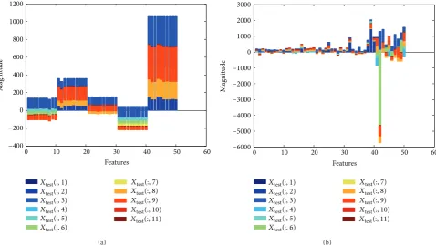
Figure 5: (a) Illustration of feature values for the RS scheme in a testing set. (b) Illustration of feature values for the OS scheme in a testing set.

After selection of the samples from each of the four segments of each and every class by the RS procedure, we combine all four samples of a class in a set called “RS” of that class and we perform similar process for the OS scheme and

called it “OS” set of that class as shown inFigure 1. Then we

extract eleven features separately from the “RS” set and the “OS” set of each class to represent the distribution pattern of that class. The reasons of considering the eleven features

in this study are discussed in detail inSection 2.2. As each

of the five classes consists of 100 single channel EEG signals,

the size of feature vector for a class is 100×11 in both the

RS and OS schemes. Thus the size of whole feature vector for

all five classes is 500×11 in both sampling processes. After

that, 10-fold cross validation process is employed to generate training set and testing set for performance evaluation of the

proposed algorithm as described inSection 3.2. In each of the

10 iterations, the training set holds 450×11 data point while

the testing set contains 50×11 data point. Here the training

set is used to train the classifier and the testing set is used to evaluate the accuracy and the effectiveness of the classifiers for the detection of the multiclass EEG data.

To provide an idea about the feature sets, we present two

diagrams: Figures5(a)and5(b)for the RS and OS scheme,

respectively, illustrating features of a testing set (1st fold). As we know, the testing set contains five class features. In both

Figures5(a)and 5(b), these five classes features are plotted

in𝑥-axis indicating 1–10 for class Z, 11–20 for class O, 21–30

for class N, 31–40 for class F, and 41–50 for class S in both figures. We observe on these two diagrams that there are some quantitative differences between two sampling (RS and OS)

features. In each classification system, the training set is fed into the three different classifiers as the input to train the classifier and the performances are assessed with the testing test.

4.2. Resultant Classification Performance. To explore the performance of the RS and OS features, we tested three

machine leaning methods:𝑘-NN, MLR with a ridge

estima-tor, and SVM for detection of multicategory EEG signals. It is important to note that, due to the usage of sampling process, different samples may come in different occasions for both the RS and OS schemes. To overcome this bias and to achieve more reliable and consistent outcomes, the sampling procedure is repeated 20 times for both the schemes with all the classifiers used in this paper and then the

average performance parameter values are reported.Table 2

reports the detection performance for the 𝑘-NN classifier

with the optimum𝑘-value (𝑘 = 1) for both the RS and OS

features, separately. This table provides different performance parameter values for each of the five classes in addition to

the overall performance. InTable 2, it can be seen that there

is a significant difference of performances of𝑘-NN classifier

between the RS and OS technique. As shown in Table 2,

under the RS scheme, all of the performances indicators demonstrate perfect detection of five categories EEG signals

by the 𝑘-NN classifier with zero FAR. In this case, all of

the measurements of TPR, precision, recall, 𝐹-value, and

accuracy for each and every class are 100% for the RS features. On the other hand, under the OS scheme, the

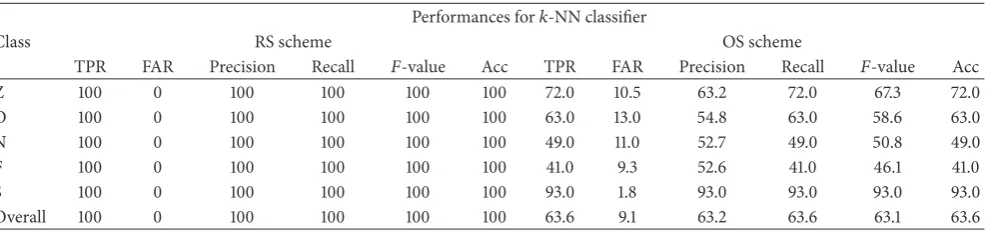
Table 2: Performances of the𝑘-NN classifier on the RS and OS scheme. Performances for𝑘-NN classifier

Class RS scheme OS scheme

TPR FAR Precision Recall 𝐹-value Acc TPR FAR Precision Recall 𝐹-value Acc

Z 100 0 100 100 100 100 72.0 10.5 63.2 72.0 67.3 72.0

O 100 0 100 100 100 100 63.0 13.0 54.8 63.0 58.6 63.0

N 100 0 100 100 100 100 49.0 11.0 52.7 49.0 50.8 49.0

F 100 0 100 100 100 100 41.0 9.3 52.6 41.0 46.1 41.0

S 100 0 100 100 100 100 93.0 1.8 93.0 93.0 93.0 93.0

Overall 100 0 100 100 100 100 63.6 9.1 63.2 63.6 63.1 63.6

Table 3: Performances of the MLR on the RS and OS scheme. Performances for MLR

Class RS scheme OS scheme

TPR FAR Precision Recall 𝐹-value Acc TPR FAR Precision Recall 𝐹-value Acc

Z 100 0 100 100 100 100 58.0 16.3 47.2 58.0 52.0 58.0

O 100 0.3 99.0 100 99.5 100 64.0 11.8 57.7 64.0 60.7 64.0

N 99.0 0 100 99.0 99.5 99.0 63.0 10.5 60.0 63.0 61.5 63.0

F 100 0 100 100 100 100 31.0 8.3 48.4 31.0 37.8 31.0

S 100 0 100 100 100 100 90.0 1.8 92.8 90.0 91.4 90.0

Overall 99.8 0.1 99.8 99.8 99.8 99.8 61.2 9.7 61.2 61.2 60.7 61.2

the overall TPR, precision, recall,𝐹-value, and accuracy for

the OS features are 63.6%, 9.1%, 63.2%, 63.6%, 63.1%, and 63.6%, respectively, with varying FAR. The overall accuracy is increased 36.4% for the RS scheme compared to the OS scheme. The significant improvement is due to the fact of the use of the RS scheme, the statistical features that well represent the EEG signals compared to the OS scheme.

Tables 3 and 4 display the classification results of the

MLR and SVM classifiers under both RS and OS approach.

In both Tables 3 and 4, it is seen that the RS technique

achieves better performances for each and every individual class with the MLR with very low FPR compared with the

OS technique. As shown inTable 3, the overall accuracy is

99.80% for the RS based MLR approach, while it is 61.20% for the OS based MLR method. In this case, the performance is

improved 38.6% for the RS scheme. We can also see inTable 4

that the RS technique achieves 99.40% of the overall accuracy for the SVM classifier whereas it is very low, 23.0%, for the OS scheme. As we can see, the RS approach consistently

performs better for the 𝑘-NN, MLR, and SVM classifiers

with very few FPR. On the other hand, the OS approach is continuously producing lower performances and higher FAR with these three classifiers. This may be due to that fact that, under the OS approach, the sampling procedures and the statistical features do not represent the whole EEG signals. According to the classification results as displayed in Tables 2–4, it is obvious that the RS process is the best way for achieving representative information from various categories

EEG signals and the𝑘-NN classifier is the top suited with the

RS based features for detecting multicategories EEG signals.

Figure 6displays kappa statistics for the𝑘-NN, MLR, and

SVM classifier under the RS and OS scheme. In this research, kappa statistics test is used to evaluate the consistency of

1 0.9975 0.9925

0.545 0.515

0.0375

0 0.2 0.4 0.6 0.8 1 1.2

k-NN MLR SVM

K

ap

p

a val

ues

Kappa statistics

RS OS −0.2

Figure 6: Kappa statistics values for the𝑘-NN, MLR, and SVM classifier under the RS and OS scheme.

the three classifiers:𝑘-NN, MLR, and SVN between the two

processes, RS and OS scheme. The consistency is mild if kappa value is less than 0.2, fair if it lies between 0.21 and 0.40, moderate if it lies between 0.41 and 0.60, good if it is between 0.61 and 0.80, and excellent if it is greater than 0.81.

As seen inFigure 6, kappa values are very high (close to 1)

for the RS scheme compared to the OS scheme for all of the three classifiers. In this figure, error bars indicate the standard error and standard errors are very high in the OS scheme for each of the three classifiers that indicate inconsistency of

the OS method. InFigure 6, it can be seen that the highest

kappa value is obtained by the𝑘-NN algorithm with the RS

scheme. This clearly indicates that the performance of the RS

scheme with the𝑘-NN classifier is excellent for the detection

Table 4: Performances of the SVM with RBF kernel classifier on the RS and OS scheme. Performances for SVM with RBF kernel classifier

Class RS scheme OS scheme

TPR FAR Precision Recall 𝐹-value Acc TPR FAR Precision Recall 𝐹-value Acc

Z 99.0 0 100 99.0 99.5 99.0 7.0 0 100 7.0 13.1 7.0

O 99.0 0 100 99.0 99.5 99.0 4.0 0 100 4.0 7.7 4.0

N 99.0 0 100 99.0 99.5 99.0 2.0 0 100 2.0 3.9 2.0

F 100 0 100 100 100 100 2.0 0.3 66.7 2.0 3.9 2.0

S 100 0.8 97.1 100 98.5 100 100 96.0 20.7 100 34.2 100

Overall 99.4 0.2 99.4 99.4 99.4 99.4 23.0 19.3 77.5 23.0 12.6 23.0

0 0.2 0.4 0.6 0.8 1 1.2

Z O N F S Overall

RO

C

are

a

MLR_RS

MLR_OS SVN_RS SVM_OS k-NN_RS

k-NN_OS

Figure 7: ROC area for the𝑘-NN, MLR, and SVM classifier with the RS and OS scheme.

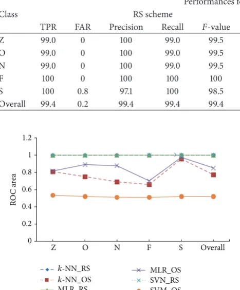
Figure 7 presents ROC areas for the 𝑘-NN, MLR, and

SVM classifiers with the RS and OS scheme, separately for each of five classes and their overall ROC area as well. The area of the ROC curve is used as an index for evaluating classifier performance (e.g., lager area indicates better performance of

the classifier). As can be seen inFigure 7, each of the three

classifiers produces higher ROC area close to 1 with the use of the RS scheme for each class while they yield lower area with the use of the OS scheme. This figure validates the reliability of the use of the RS scheme compared with the OS scheme to get representative sample point from the EEG data. The shape of the MAE for each of the three classifiers under the

RS and OS scheme is illustrated inFigure 8. It is noted that

the lower MAE score indicates the higher performance of the scheme. We can see that the score of MAE is very low for the RS approach for each of the three classifiers. On the other hand, the OS approach yields very high score of MAE for each of the classifiers. In this figure, we also observe that the lowest

MAE is produced by the𝑘-NN approach among the three

classifiers for the RS scheme. Thus we can argue strongly that the statistical features obtained from RS scheme are perfect

representation of EEG signals and the𝑘-NN classifier is the

best choice for multicategory EEG signals detection. Plenty of promising research works have been devoted to the two-class classification problems providing very good outcomes dealing with the benchmark epileptic EEG data

[18,37,42,43] but a few studies in the literature [5,6,9–11]

RS OS 0

0.05 0.1 0.15 0.2 0.25 0.3 0.35

MLR

SVM

Sc

o

re

Mean absolute error

RS OS

RS O k-NN

Figure 8: 3D stacked area graph showing MAE for the𝑘-NN, MLR, and SVM classifier under the RS and OS scheme.

(discussed inSection 1) have been performed for the

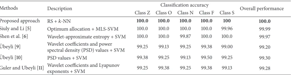
multi-class EEG signal multi-classification. In order to further examine the efficiency of our proposed framework, we also provide a comparison of our proposed approach with five

well-known reported algorithms.Table 5presents a comparative

study between our proposed method and the five reference algorithms for the same benchmark epileptic EEG dataset. This table reports the detection performances of the five categories EEG signals in terms of class specific accuracy and overall accuracy. The highest classification performances

among the five algorithms are highlighted in bold font in

each method. From Table 5, it is clear that our proposed

algorithm yields the perfect detection performances that are not achieved by any other methods in the literature. Thus, the RS scheme can be used as a perfect scheme for

feature extractions while the𝑘-NN can be considered as an

optimum choice with it for the detection of multicategories EEG signals.

5. Concluding Remarks

Table 5: Comparison the results of our proposed approach with some reported research outcomes.

Methods Description Classification accuracy Overall performance

Class Z Class O Class N Class F Class S

Proposed approach RS +𝑘-NN 100.0 100.0 100.0 100.0 100 100.0

Siuly and Li [5] Optimum allocation + MLS-SVM 100.0 100.0 100.0 100.0 99.96 99.99 Shen et al. [6] Wavelet-approximate entropy + SVM 100.0 100.0 99.87 100.0 100.0 99.97

¨

Ubeyli [9] Wavelet coefficients and power

spectral density (PSD) values + SVM 99.25 99.13 99.25 99.38 99.00 99.20 ¨

Ubeyli [10] PSD values + SVM 99.38 99.25 99.13 99.50 99.25 99.30 Guler and Ubeyli [11] Wavelet coefficients and Lyapunov

exponents + SVM 99.25 99.38 99.25 99.38 99.13 99.28

signals. The RS and OS scheme are employed to select rep-resentative samples from different segments of multicategory EEG signals. We experimented this methodology on bench-mark epileptic EEG database. To examine the consistency of the structure, the sample selection procedure in both the RS and OS schemes with all the classifiers used in this paper is repeated for 20 times and the average performance parameter values are reported. The experimental results show that the features obtained from the RS well represent the multicategory EEG signals and achieve the consistent detection rates in terms of all possible detection parameters in all of the three classifiers used in this paper. The results also

demonstrated that the𝑘-NN classifier perfectly detects (100%

for all performance indicator) the multicategory EEG signals under the RS technique. The results represent a proof concept of the successful detection of multicategory brain dynamics quantification through EEGs. Due to its perfect detection, the RS technique is strongly recommended for capturing the valuable information from the original EEG data which is best

suited with the𝑘-NN classifier. The proposed method may be

applied for analysis and classification of other nonstationary biomedical signals.

Conflict of Interests

The authors declare that there is no conflict of interests regarding the publication of this paper.

Acknowledgments

This work is supported by the National Natural Science Foundation of China (NSFC 61332013) and the Australian Research Council (ARC) Linkage Project (LP100200682).

References

[1] E. Niedermeyer and F. L. da Silva,Electroencephalography: Basic Principles, Clinical Applications, and Related Fields, Lippincott Williams & Wilkins, Philadelphia, Pa, USA, 5th edition, 2005. [2] V. Bajaj and R. B. Pachori, “Classification of seizure and

nonseizure EEG signals using empirical mode decomposition,” IEEE Transactions on Information Technology in Biomedicine, vol. 16, no. 6, pp. 1135–1142, 2012.

[3] Y. Kutlu, M. Kuntalp, and D. Kuntalp, “Optimizing the per-formance of an MLP classifier for the automatic detection of epileptic spikes,”Expert Systems with Applications, vol. 36, no. 4, pp. 7567–7575, 2009.

[4] D. Hanbay, “An expert system based on least square support vector machines for diagnosis of the valvular heart disease,” Expert Systems with Applications, vol. 36, no. 3, pp. 4232–4238, 2009.

[5] S. Siuly and Y. Li, “A novel statistical algorithm for multiclass EEG signal classification,”Engineering Applications of Artificial Intelligence, vol. 34, pp. 154–167, 2014.

[6] C.-P. Shen, C.-C. Chen, S.-L. Hsieh et al., “High-performance seizure detection system using a wavelet-approximate entropy-fSVM cascade with clinical validation,”Clinical EEG and Neu-roscience, vol. 44, no. 4, pp. 247–256, 2013.

[7] P. P. Acharjee and C. Shahnaz, “Multiclass epileptic seizure classification using time-frequency analysis of EEG signals,” inProceedings of the 7th International Conference on Electrical and Computer Engineering (ICECE '12), pp. 260–263, Dhaka, Bangladesh, December 2012.

[8] A. S. M. Muthanantha Murugavel, S. Ramakrishnan, K. Bal-asamy, and T. Gopalakrishnan, “Lyapunov features based EEG signal classification by multi-class SVM,” inProceedings of the World Congress on Information and Communication Technolo-gies (WICT ’11), pp. 197–201, December 2011.

[9] E. D. ¨Ubeyli, “Decision support systems for time-varying biomedical signals: EEG signals classification,”Expert Systems with Applications, vol. 36, no. 2, pp. 2275–2284, 2009.

[10] E. D. ¨Ubeyli, “Analysis of EEG signals by combining eigenvector methods and multiclass support vector machines,”Computers in Biology and Medicine, vol. 38, no. 1, pp. 14–22, 2008.

[11] I. Guler and E. D. Ubeyli, “Multiclass support vector machines for EEG-signals classification,”IEEE Transactions on Informa-tion Technology in Biomedicine, vol. 11, no. 2, pp. 117–126, 2007. [12] K. Polat and S. G¨unes¸, “Classification of epileptiform EEG using

a hybrid system based on decision tree classifier and fast Fourier transform,”Applied Mathematics and Computation, vol. 187, no. 2, pp. 1017–1026, 2007.

[13] S. Siuly and Y. Li, “Discriminating the brain activities for brain– computer interface applications through the optimal allocation-based approach,”Neural Computing and Applications, 2014. [14] W. G. Cochran,Sampling Techniques, Wiley, New York, NY,

USA, 1977.

[16] Sample size calculator, http://www.surveysystem.com/sample-size-formula.htm.

[17] R. D. de Veaux, P. F. Velleman, and D. E. Bock, Intro Stats, Pearson Addison Wesley, Boston, Mass, USA, 3rd edition, 2008. [18] Siuly, Y. Li, and P. P. Wen, “Clustering technique-based least square support vector machine for EEG signal classification,” Computer Methods and Programs in Biomedicine, vol. 104, no. 3, pp. 358–372, 2011.

[19] M. N. Islam, An Introduction to Statistics and Probability, Mullick & Brothers, Dhaka, Bangladesh, 3rd edition, 2004. [20] R. O. Duda, P. E. Hart, and D. G. Strok,Pattern Classification,

John Wiley & Sons, 2nd edition, 2001.

[21] Y. Song, J. Huang, D. Zhou, H. Zha, and C. L. Giles, “IKNN: informative K-nearest neighbor pattern classification,” inKnowledge Discovery in Databases: PKDD 2007, vol. 4702 ofLecture Notes in Computer Science, pp. 248–264, Springer, Berlin, Germany, 2007.

[22] J. Han, M. Kamper, and J. Pei, Data Mining: Concepts and Techniques, Morgan Kaufmann, 2005.

[23] B. D. Ripley,Pattern Recognition and Neural Networks, Cam-bridge University Press, CamCam-bridge, UK, 1996.

[24] S. L. Cessie and J. C. Van Houwelingen, “Ridge estimators in logistic regression,”Applied Statistics, vol. 41, no. 1, pp. 191–201, 1992.

[25] F. M. Zahid and G. Tutz, “Ridge estimation for multinomial logit models with symmetric side constraints,”Computational Statistics, vol. 28, no. 3, pp. 1017–1034, 2013.

[26] V. N. Vapnik,The Nature of Statistical Learning Theory, Springer, New York, NY, USA, 2000.

[27] R. K. Begg, M. Palaniswami, and B. Owen, “Support vector machines for automated gait classification,”IEEE Transactions on Biomedical Engineering, vol. 52, no. 5, pp. 828–838, 2005. [28] X. Yin, B. W.-H. Ng, B. M. Fischer, B. Ferguson, and D.

Abbott, “Support vector machine applications in terahertz pulsed signals feature sets,”IEEE Sensors Journal, vol. 7, no. 12, pp. 1597–1607, 2007.

[29] EEG time series, 2005, http://www.meb.uni-bonn.de/epilep-tologie/science/physik/eegdata.html.

[30] R. G. Andrzejak, K. Lehnertz, F. Mormann, C. Rieke, P. David, and C. E. Elger, “Indications of nonlinear deterministic and finite-dimensional structures in time series of brain electrical activity: dependence on recording region and brain state,” Physical Review E, vol. 64, no. 6, Article ID 061907, 8 pages, 2001. [31] W. A. Chaovalitwongse, Y.-J. Fan, and R. C. Sachdeo, “On the time seriesK-nearest neighbor classification of abnormal brain activity,”IEEE Transactions on Systems, Man, and Cybernetics, Part A: Systems and Humans, vol. 37, no. 6, pp. 1005–1016, 2007. [32] B. Efron, “Estimating the error rate of a prediction rule: improvement on cross-validation,”The Journal of the American Statistical Association, vol. 78, no. 382, pp. 316–331, 1983. [33] S. Siuly and Y. Li, “Improving the separability of motor imagery

EEG signals using a cross correlation-based least square support vector machine for brain-computer interface,”IEEE Transac-tions on Neural Systems and Rehabilitation Engineering, vol. 20, no. 4, pp. 526–538, 2012.

[34] A. Sengur, “Multiclass least-squares support vector machines for analog modulation classification,”Expert Systems with Appli-cations, vol. 36, no. 3, pp. 6681–6685, 2009.

[35] Siuly, Y. Li, and P. Wen, “Modified CC-LR algorithm with three diverse feature sets for motor imagery tasks classification in

EEG based brain-computer interface,”Computer Methods and Programs in Biomedicine, vol. 113, no. 3, pp. 767–780, 2014. [36] S. Faul and W. Marnane, “Dynamic, location-based channel

selection for power consumption reduction in EEG analysis,” Computer Methods and Programs in Biomedicine, vol. 108, no. 3, pp. 1206–1215, 2012.

[37] L. Guo, D. Rivero, J. A. Seoane, and A. Pazos, “Classification of EEG signals using relative wavelet energy and artificial neural networks,” inProceedings of the first ACM/SIGEVO Summit on Genetic and Evolutionary Computation (GEC ’09), pp. 177–183, June 2009.

[38] L. M. Patnaik and O. K. Manyam, “Epileptic EEG detection using neural networks and post-classification,”Computer Meth-ods and Programs in Biomedicine, vol. 91, no. 2, pp. 100–109, 2008.

[39] L. Fraiwan, K. Lweesy, N. Khasawneh, M. Fraiwan, H. Wenz, and H. Dickhaus, “Classification of sleep stages using multi-wavelet time frequency entropy and LDA,”Methods of Informa-tion in Medicine, vol. 49, no. 3, pp. 230–237, 2010.

[40] E. Frank, M. Hall, G. Holmes et al., “Weka—a machine learning workbench for data mining,” inData Mining and Knowledge Discovery Handbook, pp. 1269–1277, Springer US, 2010. [41] C. C. Chang and C. J. Lin, “LIBSVM: a library for support

vector machines,”ACM Transactions on Intelligent Systems and Technology, vol. 2, no. 3, article 27, 2011.

[42] L. Guo, D. Rivero, and A. Pazos, “Epileptic seizure detection using multiwavelet transform based approximate entropy and artificial neural networks,”Journal of Neuroscience Methods, vol. 193, no. 1, pp. 156–163, 2010.

Submit your manuscripts at

http://www.hindawi.com

Stem Cells

International

http://www.hindawi.com Volume 2014

Hindawi Publishing Corporation

http://www.hindawi.com Volume 2014

INFLAMMATION

Hindawi Publishing Corporation

http://www.hindawi.com Volume 2014

Behavioural

Neurology

Endocrinology

Hindawi Publishing Corporation

http://www.hindawi.com Volume 2014

Hindawi Publishing Corporation

http://www.hindawi.com Volume 2014

Disease Markers

Hindawi Publishing Corporation

http://www.hindawi.com Volume 2014

BioMed

Research International

Oncology

http://www.hindawi.com Volume 2014

Hindawi Publishing Corporation

http://www.hindawi.com Volume 2014 Oxidative Medicine and Cellular Longevity Hindawi Publishing Corporation

http://www.hindawi.com Volume 2014

PPAR Research

The Scientific

World Journal

http://www.hindawi.com Volume 2014

Immunology Research

Hindawi Publishing Corporation

http://www.hindawi.com Volume 2014 Journal of

Obesity

Hindawi Publishing Corporation

http://www.hindawi.com Volume 2014

Hindawi Publishing Corporation

http://www.hindawi.com Volume 2014

Computational and Mathematical Methods in Medicine

Ophthalmology

Hindawi Publishing Corporation

http://www.hindawi.com Volume 2014

Diabetes Research

http://www.hindawi.com Volume 2014

Hindawi Publishing Corporation

http://www.hindawi.com Volume 2014

Research and Treatment

AIDS

Hindawi Publishing Corporation

http://www.hindawi.com Volume 2014

Gastroenterology Research and Practice

Hindawi Publishing Corporation

http://www.hindawi.com Volume 2014

Parkinson’s

Disease

Evidence-Based Complementary and Alternative Medicine

Volume 2014