Designing a new data intelligence model for global solar radiation prediction: application of multivariate modeling scheme

Article

Designing a New Data Intelligence Model for Global

Solar Radiation Prediction: Application of

Multivariate Modeling Scheme

Hai Tao1, Isa Ebtehaj2,3 , Hossein Bonakdari2,3, Salim Heddam4 , Cyril Voyant5,6 , Nadhir Al-Ansari7 _{, Ravinesh Deo}8 _{and Zaher Mundher Yaseen}9,_*

1 _{Computer Science Department, Baoji University of Arts and Sciences, Baoji 721000, China;}

[email protected]

2 _{Department of Civil Engineering, Razi University, Kermanshah 97146, Iran; [email protected] (I.E.);}

[email protected] (H.B.)

3 _{Environmental Research Center, Razi University, Kermanshah 67146, Iran}

4 _{Faculty of Science, Agronomy Department, Hydraulics Division, Laboratory of Research in Biodiversity}

Interaction Ecosystem and Biotechnology, University 20 Août 1955, Route El Hadaik, BP 26, Skikda 21000, Algeria; [email protected]

5 _{Castelluccio Hospital, Radiotherapy Unit, BP 85, 20177 Ajaccio, France; [email protected]}

6 _{University of Reunion Island—PIMENT Laboratory, 15, Avenue RenéCassin, BP 97715 Saint-Denis CEDEX,}

France

7 _{Civil, Environmental and Natural Resources Engineering, Lulea University of Technology, 97187 Lulea,}

Sweden; [email protected]

8 _{School of Agricultural, Computational and Environmental Sciences, Centre for Sustainable Agricultural}

Systems & Centre for Applied Climate Sciences, Institute of Life Sciences and the Environment, University of Southern Queensland, Springfield, QLD 4300, Australia; [email protected]

9 _{Sustainable Developments in Civil Engineering Research Group, Faculty of Civil Engineering,}

Ton Duc Thang University, Ho Chi Minh City, Vietnam

* Correspondence: [email protected]; Tel.: +84-033-498-7030

Received: 14 March 2019; Accepted: 3 April 2019; Published: 9 April 2019

Abstract:Global solar radiation prediction is highly desirable for multiple energy applications, such as energy production and sustainability, solar energy systems management, and lighting tasks for home use and recreational purposes. This research work designs a new approach and investigates the capability of novel data intelligent models based on the self-adaptive evolutionary extreme learning machine (SaE-ELM) algorithm to predict daily solar radiation in the Burkina Faso region. Four different meteorological stations are tested in the modeling process: Boromo, Dori, Gaoua and Po, located in West Africa. Various climate variables associated with the changes in solar radiation are utilized as the exploratory predictor variables through different input combinations used in the intelligent model (maximum and minimum air temperatures and humidity, wind speed, evaporation and vapor pressure deficits). The input combinations are then constructed based on the magnitude of the Pearson correlation coefficient computed between the predictors and the predictand, as a baseline method to determine the similarity between the predictors and the target variable. The results of the four tested meteorological stations show consistent findings, where the incorporation of all climate variables seemed to generate data intelligent models that performs with best prediction accuracy. A closer examination showed that the tested sites, Boromo, Dori, Gaoua and Po, attained the best performance result in the testing phase, with a root mean square error and a mean absolute error (RMSE-MAE [MJ/m2]) equating to about (0.72-0.54), (2.57-1.99), (0.88-0.65) and (1.17-0.86), respectively. In general, the proposed data intelligent models provide an excellent modeling strategy for solar radiation prediction, particularly over the Burkina Faso region in Western Africa. This study offers implications for solar energy exploration and energy management in data sparse regions.

Keywords:energy harvesting; solar radiation simulation; SaE-ELM model; multivariate modeling; African region

1. Introduction

Since the 19th century, significant scientific efforts have been dedicated to the development of new renewable energy systems, due to growing industrialization, depleting reservoirs of fossil fuels, and modern lifestyles [1,2]. These efforts have encompassed research works in different academic fields, to involve the efforts of government and non-governmental organizations, world communities, leaders, and energy managers in a bid to make life easier and more comfortable through the provision of better energy security and management systems [3].

Renewable sources of energy have attracted much research interest in the 19th century due to emerging algorithms that lead to discoveries in new models and greater knowledge about the impact of non-renewable energies on the environment [4,5]. This interest is mainly because renewable energy is sustained by natural processes, which do not contribute towards the generation of GHGs, or related global warming and climate change issues [6]. Since the discovery of solar energy as a sustainable source of renewable energy in the mid-19th century, it has received global attention as a source of power generation to overcome issues related to fossil fuels [7].

Prediction of solar radiation is important for modern-day integrated energy management systems, as they can be operated continuously for long hours and days if they are based on solar energy; in addition, they can help overcome electrical power shortage caused by the stochastic nature of solar radiation [8]. These predictions are a crucial way to integrate solar resources into an electrical power grid and can provide energy utilities with updated and correct information on the availability of solar energy from solar radiation, which is critical to support decisions on load balancing and switching power transmissions into a distributed network. These predictions can also help dispatch power at optimal periods and facilitate the right amount of energy into a local and national power grid [9]. This can help maximize the benefit of photovoltaic storage for residential or commercial end-users to help in scheduling and coordinating end-users’ energy consumption, distributed generation, and storage [10,11]. Overall, a predictive model for solar radiation can help utilities to minimize their operational costs, improve efficiency, and provide power quality and reliability for a better energy security platform [12].

There is no doubt that the best way to generate global solar data is to use the appropriate radiometric instrument to directly measure solar data at a specific solar energy site. Owing to the cost implications of this method and the required expertise for ground and satellite-based measurement of global solar radiation, most countries in Africa and Asia have limited radiometric data [13]. Moreover, some stations that measure global stations concentrate on urban towns and cities, neglecting rural areas, where the energy crisis is more prominent. Most of the government-owned metro stations in Burkina Faso lack the capacity to measure routine globe solar radiation data [14]. However, areas with readily available data suffer from incomplete monthly or daily radiometric data due to improper equipment calibration. Another way to generate solar radiation is through Meteoblue, a “meteorological reanalysis” approach [15]. This is a physically-based simulation of meteorological parameters by a physical model (5 km × 5 km) based on Nonhydrostatic Meso-Scale Modelling (NMM) technology that uses topography, coverage, and soil. Despite the benefits it may offer, such as incorporating physical processes that affect ground-based solar radiation, the values generated by the Meteoblue approach are simulated rather than real. These simulations include the use of mathematical equations that are forced on the prescribed initial and model boundary conditions; hence, the forecasts may differ from those physically observed at a station on the ground [16].

and temperature are likely to govern changes in solar radiation. Hence, quantifying solar radiation is a difficult problem and solving this issue has been attracting the attention of research scholars for many decades. Traditionally, solar radiation is calculated with multiple manual and empirical formulations [6,17], including the Meteoblue, a “meteorological reanalysis” approach [16]. However, these studies can have several limitations based on empirical formulas or complex mathematical equations. For different case study regions, the initial conditions forced onto physical models may not adequately address the particular behaviors and variations in the results due to the high stochasticity of variables related to solar radiation incorporated with actual data. Hence, the motivation of renewable energy scientists is to determine new alternative modeling strategies to resolve this problem.

The application of artificial intelligence (AI) have been massively explored for solar radiation modeling over the past two decades [18]. Several models have been applied to mimic the actual pattern of solar radiation using artificial neural network (ANN) [19–21], fuzzy set models [22–24], genetic programming [25–27], support vector machine (SVM) [28–30], and other kinds of complementary (or hybrid) predictive models [31–33]. Despite massive implementation of data intelligent models, multiple drawbacks have been identified through several review researches, such as poor prediction for dataset, which is not in range of the learning values, incorporation of error through the modeling phase, requirement of long time series data for model training and testing, and tuning of multiple internal parameters [17,34,35]. These artificial intelligence models are often taken together as a whole or hybridized to eliminate weaknesses of individual models.

However, the hybrid technique of prediction global solar radiation using regression models alone is more suitable compared to its single parameter based-model counterpart [30,36,37]. Solar energy researchers have introduced powerful hybrid soft computing techniques with a high level of accuracy, precision, reliability, and adaptability. These techniques have proven to yield outstanding prediction accuracy owing to their ability to integrate different AI with natural inspired optimization algorithms [38–40].

The firefly evolutionary algorithm within support vector machines (SVM-FFA) was employed to predict global solar radiation at Iseyin, Maiduguri, and Jos located in Nigeria using sunshine duration, and maximum and minimum temperature as input parameters [30]. The authors validated the initiated technique by comparing it with ANN and genetic programming technique. The results revealed that the novel SVM-FFA technique yielded more precise predictions compared to ANN and GP techniques in the three locations. Another attempt was established by applying grouping genetic algorithm (GGA) evolutionary extreme learning machine (ELM), (GGA-ELM) and traditional ELM to predict global solar radiation using numerical weather model input at Toledo’s radiometric observatory, Spain [36]. The GGA-ELM has shown excellent performance in the evaluated statistical indicators, compared to traditional ELM. A novel Coral Reefs Optimization-Extreme Learning machine (CRO-ELM) and conventional extreme learning machine (ELM) techniques have inspected data patterns to predict the changes in global solar radiation, by applying various meteorological parameters in Murcia, southern Spain [41]. The results show that the novel CRO-ELM performed better than the traditional ELM technique. Adaptive neuro fuzzy inference system (ANFIS) was tuned using FFA optimizer for solar radiation prediction using different climate information over China [42]. The proposed hybrid ANFIS-FFA model demonstrated excellent performance predictability against the empirical formulations for day of the year modeling scheme solar prediction.

in the literature [45]. However, the capabilities of self-adaptive operators is another new evolutionary case of computing that is lacking in literature works focusing on feature selection problems [39,46,47]. In the recent decade, a suite of evolutionary algorithms has been broadly utilized as global search techniques to optimize the parameters of artificial intelligence-based techniques. One of the most popular evolutionary algorithms is differential evolution (DE) [48]. DE is a powerful and simple population-based stochastic direct searching approach. It is mostly used to optimize selection of the network parameters. In all combinations of artificial intelligence-based techniques with DE, the control parameters and strategies of trial vector generation of the DE algorithm must be manually selected through a trial-and error-process. As pointed out in different DE-based studies, the performance of DE is highly dependent on the selection of the mentioned strategies and control parameters, such that unsuitable selections of control parameters and strategies may lead to stagnation or premature convergence. Therefore, to apply DE to different problems, fixing control parameters and strategies of the trial vector generation may also result in different network generalization performances.

In this study, a self-adaptive evolutionary extreme learning machine as a new novel case of ELM model was developed to predict global solar radiation for the African region. In this evolutionary based method, the hidden nodes of the single layer feedforward network are optimized by the self-adaptive differential evolution algorithm. Indeed, the control parameters and strategies are self-adapted in a strategy pool using former experiences in producing promising solutions. Besides, the output weights in this network are computed by the Moore—Penrose generalized inverse. While some soft computing algorithms need the adjustment of various variables to obtain results, the SaE-ELM algorithm needs no pre-specific knowledge of control variables, hence resulting in less influence of the optimization problem.

The main objective of this research paper is to determine the capacity of the newly initiated hybrid SaE-ELM for prediction of global solar radiation on the horizontal surface in Burkina Faso. To realize this, four different meteorological stations distributed across Burkina Faso have been used to quantify the impact of meteorological variables on the capacity of the newly initiated technique. Eight different models were developed using wind speed, maximum and minimum temperature, maximum and minimum humidity vapor pressure, and eccentricity correction factor due to the availability and completeness of data in the meteorological station in Burkina Faso. This research anchors on the necessity of reliable global solar radiation data utilization for agricultural, hydrological and ecological applications for prediction of energy output of solar system in the Burkina Faso region, where the energy crisis is high.

2. Methods and Materials

2.1. Self-Adaptive Evolutionary Extreme Learning Machine

The SaE-ELM method comprises of two integrated components—The extreme learning machine (ELM) regression method and the self-adaptive version of the differential evolution (DE). In the following section, a brief overview is provided for the ELM and adaptive differential; interested readers can find more details in [49]. Following the brief on both components, their integration within the SaD-ELM procedure is discussed.

2.2. Extreme Learning Machine (ELM)

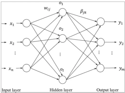
neural network that is suitable for applicable problems. According to Figure1, the ELM structure has a full connection between the input-to-hidden and hidden-to-output layer. The input layer has nneurons, which are equal to the number of input variables of the considered problem. Similarly, the output layer hasmneurons, which are equal to the number of output variables of the considered problem. There is no method to determine the hidden layer’s neuron numbers and it is done by considering the difficulty level of the problem. However, the high number of hidden nodes may be lead to overfitting. Therefore, through the training phase and due to complexity of the model, the number of neurons should be selected in such a way that not only is their number not high, but the models should also provide accurate results. In this study, the number of hidden nodes is considered as 30 for all models.

Figure 1.Structure of the classic extreme learning machine predictive model.

Due to the ELM structure in Figure1, for an ELM network withlhidden layer neuron, the weigh matrix between the input and hidden layer that linked theith neuron of the input layer to thejth neuron of the hidden layer is defined asw= [wij]n×l(n is the number of input variables). Another weight matrix in the ELM network isβ= [βjk]l×mwhich links thejth neuron of the hidden layer to the kth neuron of the output layer. If we consider Q as an input samples number, the input and output matrices are defined asX= [xij]n×QandT= [tij]m×Q, respectively. By consideringg(x) as an activation function, the target matrix of the ELM network is presented as follows:

Tj=

     

t1j

t2j .. . tmj      

m×1 =             l ∑

i=1

βi1g[wixi+bi] l

∑

i=1

βi2g[wixi+bi] ..

. l

∑

i=1

βimg[wixi+bi]

           

m×1

, (j=1, 2, . . . , Q) (1)

There are many activation functions, which include hard limit, triangular basis function, radial basis function, sine, and sigmoid. The sigmoid activation function [50–52] is employed in this study due to its successful performance in recent studies. The above-mentioned equation could be presented in the matrix form, as follows:

whereTis the target matrix,βis the weight matrix between hidden and output layers, andHis calculated as: H=      

g[w1x1+b1] g[w2x1+b2] · · · g[wlx1+bl] g[w1x2+b1] g[w2x2+b2] · · · g[wlx2+bl]

..

. ... ...

g

w1xQ+b1 gw2xQ+b2 · · · gwlxQ+bl

     

Q×l

(3)

If the number of hidden layer neurons (l) is considered equal to the number of problem samples (Q), the best ELM results are obtained. It should be noted that the high number of hidden layer neurons results in a very complicate and big model and the probability of overfitting is high. Therefore, the number of hidden layer neurons is considered much lower than the number of problem samples. Consequently, the trained ELM model has aε> 0 (εis the defined error) as:

Q

∑

<ε (4)

Due to random selection of the b and w parameters, theβmatrix is calculated bymin

β

Hβ−TT.

By defining the Moore-Penrose generalized inverse matrix ofH(H+), the solution of this equation is obtained as ˆβ=H+TT.

2.3. Differential Evolution (DE)

The DE optimization algorithm was introduced by Storn and Price [45] as a global search method to optimize the network parameters. This algorithm has a high convergence speed and automatic exploration-exploitation adjustability. The goal of DE is to minimize the objective functionf(θ), where θis the parameter vector. In search for the optimum solution, the DE generatesNppopulations. At the Gth generation, theith parameter vector is written as:

θi,G =

h

θ1_i.G,θ_i2_.G, . . . ,θ_iD_.G

i

, wherei=1, 2, . . . , Np (5)

whereDis the dimension of the problem. The DE algorithm is presented in [52]. However, the main steps of this algorithm are presented here briefly [53]:

1. Initialization of problem: NumberNpparameter vectorsθi,Gare generated randomly through the following equation:

θi,G =θmin+rand(0, 1).(θmax−θmin), where 

 

 

θmin=θ_min1 ,θ_min2 , . . . ,θ_minD

θmax=θ1max,θmax2 , . . . ,θmaxD

(6)

In this equation,θminandθmaxare the bounds of the considered parameters.

2. Mutation: There are various mutation strategies [45] that can be applied to produce mutant vector νi,Gfor each individual parameter vectorθi,G. While there are many mutation strategies, four are utilized here:

Strategy 1 : νi,G=θ_ri

1,G+F.

θ_ri

2,G−θri3,G

(7)

Strategy 2 : νi,G =θ_ri

1,G

+F.θbest,G−θ_ri

1,G

+F.θ_ri

2,G−θr3i,G

+F.θ_ri

4,G−θri5,G

(8)

Strategy 3 : νi,G =θ_ri

1,G

+F.θ_ri

2,G−θri3,G

+F.θ_ri

4,G−θr5i,G

(9)

Strategy 4 : νi,G=θ_i,G+F.

θ_ri

1,G−θi,G

+F.θ_ri

2,G−θri3,G

whereFis the mutate factor,ri_kare integers obtained randomly within the range [1,2, . . . ,Np] interval. The first two strategies are suitable for solving multi-modal problems with strong exploration capacity. However, they demonstrate slow convergence speed and sometimes get stuck at local optimum. The third and fourth strategies lead to better perturbation with an associated computation cost.

3. Crossover: The crossover procedure is performed on the mutated vectors to increase mutant vectors’ diversity. At generationG, for each mutant vectorν_i,G =ν_i1_.G,ν_i2_.G, . . . ,ν_iD_.G, a trial vector ofui,G =u1i.G,u2i.G, . . . ,uDi.G

is generated using the crossover as follows:

u_ij_,G=



 

 

ν_ij_,G, ifrandj ≤CRor{j=j_rand

θ_ij_,G, Otherwise

(11)

In the above equation,CRis the crossover coefficient used to control the fraction of the parameters copied from the mutant vector and has a value between 0 and 1. Thejrandis a random integer with

value between 1 toD, which is used in order to ensure that at least one of theu_i,G parameters is different fromθ_i,G.

4. Selection: This is the final step in the DE algorithm that is used to find the individual vectors with minimum error, according to a defined fitness function.

Steps (2) to (4) are repeated to reach the defined precision or the maximum number of iterations.

2.4. SaE-ELM Model

To optimize the ELM network, the self-adaptive version of the DE was employed by Cao et al. [48] to introduce the self-adaptive evolutionary ELM (SaE-ELM). Indeed, the self-adaptive DE is used optimize hidden node biases and input weights, which are randomly selected in the ELM network and therefore can provide a robust predictive model for solar radiation.

The initial training step in SaE-ELM is generation of the initial population asNPvectors using the self-adaptive DE algorithm:θk,G =

h

aT_1,[k,G],· · ·,aT_L,[k,G],b_1,[k,G],· · ·,b_L,[k,G]i. To calculate output weight matrix, theβk,G = Hk+,GTequation should be solved. In this equation,H

+

k,Gis known as the generalized inverse ofHk,Gwhich is defined as:

H_k,G =



   

gha1,[k,G],b1,[k,G],x1 i

· · · ghaL,[k,G],bL,[k,G],x1 i

..

. . .. ...

gha_1,[k,G],b_1,[k,G],xN

i

· · · gha_L,[k,G],b_L,[k,G],xN

i      (12)

Through the evolutionary training stage, the Root Mean Squared Error (RMSE) of each individual is computed as:

RMSEk,G =

v u u u u t N ∑

i=1 L ∑

j=1

βjg

aj,|k,G|,bj,|k,G|,xi −ti

m×N (13)

TheRMSEof the initial population is saved, such that the performance of the next generation is evaluated using the following equation and compared with the previous generation:

θk,G+1= 

 

 

uk,G+1 ifRMSEθk,G−RMSEθk,G+1 >ε.RMSEθk,G

uk,G+1 if

RMSEθk,G−RMSEθk,G+1

<ε.RMSEθk,Gand

βuk,G+1

<

βθk,

θk,G else

Using the four strategies (Equations (7)–(10)), the trial vector of the self-adaptive DE algorithm is produced for each target vector.

A probability procedurePl,G (probability of thelth strategy (l= 1, 2, 3, 4) is selected in theGth generation) is defined to choose the strategy of each generation. ThePl,Gis calculated as:

Pl,G =

∑G−1

g=G−Pnsl,g

∑4

l=1Sl,G

∑G−1

g=G−Pnsl,g+∑gG=−G1−Pn fl,g

(15)

Here,n fl,gandnsl,gare the numbers of trial vectors produced at thegth generation by thelth strategy that enter into and arrive (respectively) from coming generations,CRandFare DE parameters selected from a normally distributed function for each target vector andεis a positive constant to avoid the zero-enhancement rate. The trial vector generation for the next generation is performed by θk,G+1(Equation (14)). The evolutionary process at SaE-ELM is continued until the required fitness

values is attained.

2.5. Case Study and Data Description

The present study was established in the Burkina Faso region located in Sub-Saharan Africa. About 70% of the total power generation capacity in Burkina Faso is largely sourced from thermal-fossil fuel, while hydro-power accounts for the remaining 30% [54]. Owing to the increasing cost of production, instability of oil prices, and the ever-increasing demand for electricity, the country recently installed a generating capacity of 247 MW, with 215 MW sourced from 28 fossil fuel-powered stations. The net energy import of the country from its neighboring countries currently stands at about 20%. However, remote villages have fuelwood, charcoal, agricultural residues and animal dung as their major source of energy [4]. Therefore, the opportunity to develop a new solar energy forecasting method can help the regional government in exploring solar energy as an alternative renewable resource.

In the present study, the prediction power of new machine learning predictive model called self-adaptive differential extreme learning machine was investigated. To nail this purpose, the prediction of daily solar radiation was applied as a dependent variable of four stations, namely Bormo, Dori, Gaoua, and Po, as displayed in Figure2. The input predictor variables include wind velocity (WS), maximum and minimum weather temperature (Tmaxand Tmin), maximum and minimum weather

humidity (Hmaxand Hmin), vapor pressure deficit (VPD), and evaporation (Eo). VPD is defined as

3. Application Results and Analysis

3.1. Overall Models Evaluation

In this study, daily solar radiation measured at four weathers stations in Burkina Faso was predicted using a new machine learning algorithm—The self-adaptive evolutionary extreme learning machine (SaE-ELM). The SaE-ELM was developed using a multivariate modeling scheme in which seven meteorological variables are used as inputs, e.g., maximum and minimum temperature (Tmax,

Tmin), maximum and minimum relative humidity (RHmax, RHmin), wind speed (WS), vapor pressure

deficit (VPD), and evaporation (Eo), served as the predictors. The predictive capacity of these models

were evaluated using the performance indices, namely, the correlation coefficient (R), the Nash-Sutcliffe efficiency (NSE), mean absolute error (MAE), root mean square error (RMSE), scatter index (SI), and variance accounted factor (VAF) [55].

The results are discussed below. We evaluated several input combinations of the meteorological variables and compared eight scenarios (Table1). The predicted values of the performance indices in the training and testing phases are shown in Tables2–5, respectively. According to the results obtained, several conclusions can be drawn. Firstly, the comparative results of the eight applied models (M1 to M8) revealed that model M5, which has six inputs variables (WS, Tmax, Tmin, RHmin, VPD and

Eo), yielded the best accuracy among all the developed models, and outperformed the others seven

models in term of higher R, NSE, VAF and lower RMSE, MAE and SI, at the three stations (Boromo, Gaoua and Po). At the Dori station, models M5 and M6 had a relatively similar level of accuracy in the testing phase. Secondly, regarding the importance of the seven meteorological variables, it is clear from the obtained results that model M2 in which evaporation (Eo) is removed from the inputs variables,

offers low accuracy and poor performance; it is, therefore, necessary to take into account the Eoas a

relevant input variable for predicting daily SR. Thirdly, the lowest accuracy was obtained at the Dori station, both for the training and testing phases; it is, however, important to highlight the fact that the obtained results at the Dori station, in terms of R, NSE, VAF, RMSE, MAE and SI, reveal only small and negligible differences between the eight models (M1 to M8).

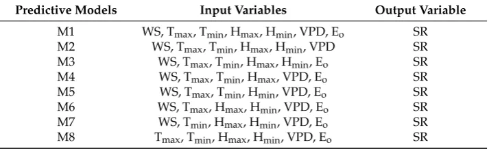
Table 1. The proposed input combination variables used as predictors attributes for solar irradiation prediction.

Predictive Models Input Variables Output Variable

M1 WS, Tmax, Tmin, Hmax, Hmin, VPD, Eo SR

M2 WS, Tmax, Tmin, Hmax, Hmin, VPD SR

M3 WS, Tmax, Tmin, Hmax, Hmin, Eo SR

M4 WS, Tmax, Tmin, Hmax, VPD, Eo SR

M5 WS, Tmax, Tmin, Hmin, VPD, Eo SR

M6 WS, Tmax, Hmax, Hmin, VPD, Eo SR

M7 WS, Tmin, Hmax, Hmin, VPD, Eo SR

M8 Tmax, Tmin, Hmax, Hmin, VPD, Eo SR

3.2. Model Comparison and Prediction Accuracy

the MAE ranges from 0.544 (MJ/M2) to 2.093 (MJ/M2) with an average of 1.181 (MJ/M2) in Boromo, from 0.657 (MJ/M2) to 2.003 (MJ/M2) with an average of 1.215 (MJ/M2) in Gaoua, and from 0.869 (MJ/M2) to 2.339 (MJ/M2) with an average of 1.342 (MJ/M2) in Po. According to the results reported in Tables2–5, it is clear that the accuracy of the eight models (M1 to M8) at the Dori station is not as good as the accuracy at Boromo, Gaoua and Po, but it is still acceptable when considering only the R and NSE values. It is clearly evidenced that the climate of Dori station, which is located at the northern east of the Burkina Faso region, is influenced by the climate of other neighbouring countries. Thus, more related information of climate variability is missing.

At the Dori station, the R ranged from 0.743 to 0.786 with an average of 0.760, and the NSE ranged from 0.479 to 0.538 with an average of 0.513. According to Legates and McCabe [56] and Moriasi et al. [57], values of R and NSE greater than 0.70 and 0.5, respectively, are considered acceptable. As stated above, the results showed that model M5 that uses WS, Tmax, Tmin, RHmin, VPD, and Eoas input variables

provided the best accuracy at Boromo, Gaoua and Po stations, while M2 in which the evaporation (Eo) is excluded from the inputs variables provided the lowest accuracy. This statement indicated that

RHmaxplayed a minor role and Eois the most important explanatory variable.

It is also important to note that by analyzing the results of Tables2–5and by comparing the performances of the M1 and M8 models, it is clear that by excluding wind speed (WS) from the inputs variables, the performance of the models significantly decrease. Hence, on one hand, increasing the number of inputs variables does not necessarily leading to better model performance in the case of RHmax; inversely, when the variable is included, the performances is lower. On the other hand,

the performance of the models decrease quickly with the exclusion of the WS variable.

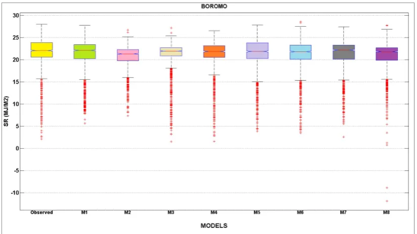
3.3. Usefulness and Assessment of the Developed Models For the Boromo station (Table2), we can see that:

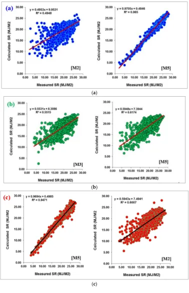
(i) The statistical indices calculated for the eight models (M1 to M8) show that the accuracy achieved using the M5 model is much higher than that achieved using the all other models with higher R, NSE and VAF values and lower MAE, RMSE and SI values. Specifically, the R, NSE, and VAF computed for M5 model are 0.982, 0.963 and 96.49, respectively. The RMSE, MAE, and SI computed for M5 model are 0.723, 0.544 and 0.034, respectively

(ii) The M5 model has the best prediction accuracy, the M1 model is the second most accurate regarding the R, VAF and MAE indices, and is followed by the M4 and M6 models. However, comparing M1, M4 and M6 models with each other only reveals small and negligible differences in corresponding statistical indices.

Slight difference between the models M4 and M6 is evident, on one hand, and model M1, on the other hand. According to Table2, at the Boromo station, the M2 model has the lowest predictive accuracy when judged by all the six statistical indices and we conclude that when Eois removed

from the inputs variables, the performances are lower. For numerical comparison, the adaptation of the Eo variable as input yielded a high and best improvement of the M1 model, compared to

the M2 model, improving its accuracy by increasing the values of the R, NSE and VAF by 24.4%, 44.5% and 40.10%, respectively, and decreasing the values of the RMSE, MAE and SI by 44.94%, 44.62% and 44.70 %, respectively (models M1 and M2). For further analysis, when looking at the WS variable, it is clear that by excluding this variable from the inputs, the quality and performances of the models significantly decreased. Nevertheless, by exclusion of the WS from the inputs of the model M1, its performances decrease significantly: the values of R, NSE and VAF decreased by 9.2%, 18.4% and 16.44%, respectively, and the values of the RMSE, MAE and SI increased by 62.22%, 68.09% and 62.71 %, respectively (models M1 and M8).

It is possible to argue that removing one or other variable does not necessarily lead to a decrease in the performances of the models; inversely, as is stated above, when RHmaxis excluded from the

exclusion of RHmaximproves the performance of the model M5 by increasing the values of R, NSE and

VAF by 3.5%, 6.9% and 7.6%, respectively, and decreasing the values of RMSE, MAE and SI by 57.20%, 58.24% and 57.62 %, respectively (models M1 and M5).

Table 2.Performance of the prediction skills of the proposed predictive model over the training and testing phase for the Boromo meteorological station (in bold, the best results for each error metrics).

Modeling Phases Input Combinations R VAF RMSE MJ/m2 _{SI MAE MJ/m}2 _Nash

Training Phase

M1 0.930265 86.52017 1.392039 0.06799 1.036243 0.846698 M2 0.634822 40.27061 2.939233 0.143559 2.078975 −0.54626 M3 0.897076 80.43472 1.679704 0.082041 1.266132 0.763912 M4 0.922551 85.07675 1.463148 0.071464 1.103346 0.829432 M5 * 0.970676 94.22108 0.907215 0.044310 0.643799 0.938422

M6 0.924674 85.49192 1.43643 0.070159 1.069989 0.833261 M7 0.900707 81.12358 1.640405 0.080121 1.280761 0.769113 M8 0.838359 70.27836 2.074775 0.101337 1.555200 0.579304

Testing Phase

M1 0.946649 89.5884 1.267718 0.059127 0.934415 0.871137 M2 0.703431 49.4815 2.821365 0.131589 2.092861 −0.01726 M3 0.921115 84.75038 1.545464 0.072081 1.174501 0.792653 M4 0.944293 89.10558 1.293015 0.060307 0.963948 0.862591 M5 * 0.982320 96.49205 0.722620 0.033703 0.54431 0.962551

M6 0.944095 89.12162 1.262830 0.058899 0.949363 0.872311 M7 0.914085 83.55511 1.557891 0.072661 1.224900 0.797607 M8 0.855340 73.13868 2.056710 0.095926 1.570392 0.596186

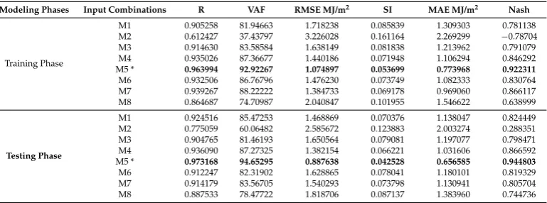
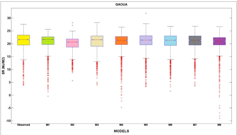
At the Gaoua station, it can be seen (Table3) by comparing the performances of the eight models, that model M5 yields higher accuracy with R, NSE and VAF equal to 0.973, 0.945 and 94.65, respectively. It can be seen that in term of RMSE, MAE and SI, the values provided with the M5 model were 0.888, 0.657 and 0.043, respectively. The M4 model is the second most accurate, and this is followed by the M1 model. The lowest accuracy was obtained by the M2 model, in which the Eovariable is excluded,

similar to the results obtained at the Boromo station. Comparing the two models M6 and M7 models reveals only small and negligible difference in corresponding statistical indices. By comparing the performances of the M6 and M7 model with the performances of the M1 model, we conclude that Tmaxand Tminhad a generally marginal effect and the two models have similar overall performances.

For example, exclusion of the Tminfrom the inputs of the M1 model decreased the values of R, NSE

and VAF by 1.2%, 3.5% and 3.15%, respectively, and increased the values of RMSE, MAE and SI by 10.90%, 3.70% and 11.42 %, respectively (models M1 and M6). Similarly, exclusion of the Tmaxfrom the

inputs of the M1 model decreased the values of R, NSE and VAF by 1.1%, 1.5% and 1.90%, respectively, and increased the values of RMSE, MAE and SI by 4.83%, 0.00% and 1.5 %, respectively (models M1 and M7). Regarding vapor pressure deficit (VPD), it is clear from the reported results that adding the VPD to the inputs of the M1 model yielded significant improvement in its performance, compared to the M3 model, with respect to all the statistical indices. The Model M1 increased the R, NSE and VAF of the M3 model by 2%, 4% and 4.01%, respectively.

Table 3.Performance of the prediction skills of the proposed predictive model over the training and testing phase for the Gaoua meteorological station.

Modeling Phases Input Combinations R VAF RMSE MJ/m2 _{SI MAE MJ/m}2 _Nash

Training Phase

M1 0.905258 81.94663 1.718238 0.085839 1.309303 0.781138 M2 0.612427 37.43797 3.226028 0.161164 2.269299 −0.78704 M3 0.914630 83.58584 1.638149 0.081838 1.213962 0.791079 M4 0.935026 87.36677 1.440186 0.071948 1.106294 0.846292 M5 * 0.963994 92.92267 1.074897 0.053699 0.773968 0.922311

M6 0.932506 86.76796 1.476230 0.073749 1.082333 0.830764 M7 0.939267 88.22222 1.384733 0.069178 0.969060 0.866117 M8 0.864687 74.70987 2.040847 0.101955 1.546622 0.638999

Testing Phase

M1 0.924516 85.47253 1.468869 0.070376 1.138047 0.824449 M2 0.775059 60.06482 2.585672 0.123883 2.003274 0.288351 M3 0.904765 81.46193 1.650564 0.079081 1.197077 0.798471 M4 0.936090 87.27325 1.382154 0.066221 1.031606 0.866592 M5 * 0.973168 94.65295 0.887638 0.042528 0.656585 0.944803

Table 4.Performance of the prediction skills of the proposed predictive model over the training and testing phase for the Dori meteorological station (in bold, the best results for each error metrics).

Modeling Phases Input Combinations R VAF RMSE MJ/m2 _{SI MAE MJ/m}2 _Nash

Training Phase

M1 0.596761 35.57581 3.270526 0.163387 2.313368 −0.89387 M2 0.594052 35.25946 3.274283 0.163575 2.303824 −0.91372 M3 0.597315 35.52598 3.277209 0.163721 2.280505 −1.01668 M4 0.603950 36.45145 3.243024 0.162013 2.308895 −0.80852 M5 * 0.623858 38.83679 3.188808 0.159305 2.226632 −0.70002

M6 0.606662 36.7405 3.250603 0.162392 2.251397 −0.82816 M7 0.588002 34.45429 3.305049 0.165112 2.302701 −1.08256 M8 0.587828 34.50788 3.298918 0.164805 2.328470 −0.99684

Testing Phase

M1 0.755305 57.02155 2.658639 0.127379 2.071896 0.190999 M2 0.757493 57.37163 2.628870 0.125953 2.039391 0.217939 M3 0.742638 55.15065 2.734910 0.131034 2.136888 0.169523 M4 0.750326 56.29248 2.650699 0.126999 2.018881 0.189014 M5 0.770053 59.29803 2.598160 0.124482 1.980505 0.285795 M6 * 0.785724 61.65339 2.576907 0.123463 1.999371 0.290784

M7 0.758246 57.48502 2.679643 0.128386 2.076499 0.213567 M8 0.766539 58.72635 2.622059 0.125627 2.037424 0.236006

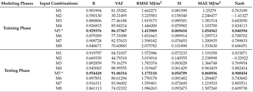
At the Po station, as seen in Table5, the present results show that the M5 yields higher accuracy with R, NSE and VAF equal to 0.954, 0.906 and 91.065, respectively. It can be seen that in terms of RMSE, MAE and SI, the values provided for the M5 model were 1.175, 0.869 and 0.055, respectively. The M2 model has the lowest accuracy, with R and NSE below 0.67 and 0.38, respectively, and a VAF value equals 44.79, highlighting the poor performances of the M2 model. Comparing the performances of the M5 and M2 models, we conclude that: (i) R, NSE, and VAF are significantly improved with increase of 28.5%, 46.27% and 52.9%, respectively. RMSE, MAE and SI are reduced by 61.07%, 62.84% and 60.99%, respectively. These results reveal significant superiority of the M5 model.

Finally, the Dori station is a particular case in which the obtained results reveal very similar performances between all the eight models. While the overall statistical indices appear to be relatively equal, the M6 model slightly outperforms the other models and has the best accuracy with high R, NSE and VAF and lower RMSE, MAE and SI values. This best can be explained owing to the fact that solar radiation magnitude is more influenced by the maximum and the minimum values of weather humidity.

Table 5.Performance of the prediction skills of the proposed predictive model over the training and testing phase for the Po meteorological station.

Modeling Phases Input Combinations R VAF RMSE MJ/m2 _{SI MAE MJ/m}2 _Nash

Training Phase

M1 0.901994 81.35282 1.662271 0.081599 1.25279 0.763189

M2 0.550130 30.21495 3.225583 0.158340 2.246477 −1.41327

M3 0.880806 77.46188 1.819173 0.089301 1.381514 0.683050

M4 0.926815 85.84214 1.446000 0.070982 1.103700 0.824113

M5 * 0.929376 86.37367 1.413969 0.069410 1.054562 0.840394

M6 0.879309 77.31098 1.831663 0.089914 1.295713 0.708702

M7 0.908728 82.57633 1.598182 0.078453 1.200935 0.789833

M8 0.840671 70.60883 2.075782 0.101898 1.533630 0.606051

Testing Phase

M1 0.919797 84.51837 1.572986 0.073233 1.191058 0.815071

M2 0.669339 44.79318 3.019014 0.140555 2.338998 −0.22922

M3 0.892859 79.16279 1.783374 0.083028 1.366748 0.769954

M4 0.945065 88.99555 1.319447 0.061429 0.963419 0.882414

M5 * 0.954428 91.06514 1.175110 0.054709 0.868936 0.900454

M6 0.897851 80.61294 1.750178 0.081482 1.284407 0.743682

M7 0.916311 83.96002 1.559401 0.072600 1.219533 0.805511

M8 0.861113 74.02332 1.986263 0.092473 1.507260 0.609738

results, the proposed SaE-ELM model indicates a feasible evolutionary intelligence model that can be utilized for solar radiation prediction as an alternative to traditional empirical equations.

Figure 3.Scatter plot evaluation over the test modeling phase for the best and worst input combinations at (a) Boromo, (b) Dori, (c) Gaoua and (d) Po meteorological stations.

Figure 5.Box plot indicator for all the inspected input combinations over the test modeling phase at the Dori meteorological station.

Figure 7.Box plot indicator for all the inspected input combinations over the test modelling phase at the Po meteorological station.

Figure 9.Violin plots indicator for all inspected input combinations over the test modelling phase at the Dori meteorological station.

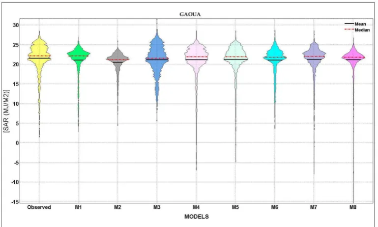
Figure 11.Violin plots indicator for all inspected input combinations over the test modelling phase at the Po meteorological station.

In spite of the good accuracy of SaE-ELM attained for the prediction of solar radiation, there exist further opportunities such as integrating this method with a physically-based method proposed by Meteoblue, a “meteorological reanalysis” approach [16]. A further study can consider the combined use of data-driven methods proposed in this paper together with the physically-based simulations by Nonhydrostatic Meso-Scale Modelling (NMM) technology, which uses topography, coverage and soil, and a suite of mathematical equations. In such an approach, the use of both data patterns as well as mathematical equations in Meteoblue method may help improve the forecasts that may not be attained by any individual method. While this is an interesting research agenda, and must be carried out, it was beyond the scope of the present study, and is highly recommended in future studies.

While evolutionary models have been known since many years and its performance in this particular study has been significantly good, the coupling of this approach with recently developed tools such as deep learning combined with evolutionary methods has rarely been used for global solar radiation prediction. Therefore, as a future study, the utilization of deep learning, combined with such evolutionary models, can potentially lead to improved prediction of solar radiation, especially when a clear sky model is not well-defined in terms of its initial conditions [38]. In order to explore deep learning with the present and other evolutionary methods for solar radiation forecasting, further research is required; for instance, by comparing the SaE-ELM forecasts with some of these other methods (e.g., Long Short-Term Memory Networks or Convolutional Neural Networks) and also studying different time forecast horizons to construct a reliable forecasting model for a robust energy security platform that integrates solar energy into a practical power grid system. While this research is an interesting endeavor, it is beyond the scope of this study, and awaits another independent investigation.

3.4. The Modeling Uncertainty Analysis

process on the investigated application. The uncertainty analysis is computed through univariate error prediction:

ej =Pj−Tj (16)

The mean and standard deviation prediction error are computed based on the error of the entire testing dataset. The mean error and standard deviation prediction error are expressed in the following formulas:

e=

∑

Se=

s

∑

(ej−e)2

n−1 (18)

The negative and positive magnitudes of the errors are denoted as under- and over-prediction values, respectively. The mean and standard deviation error is utilized to generate the confidence band around the predicted values based on Wilson metrics [46]. The best input combination of each investigated station using SaE-ELM demonstrated a persuaded level of mean prediction error.

Table 6.Uncertainty analysis for the developed SaE-ELM based models at all meteorological stations (in bold, the lowest values).

Meteorological Station Input Combinations Mean Prediction Error Standard Deviation of Prediction Error

Width of Uncertainty Band

95% Prediction Error Interval

Bormo

Model 1 1.280 1.537 ±0.300 (0.980, 1.581)

Model 2 2.049 1.893 ±0.370 (1.679, 2.419)

Model 3 1.488 1.947 ±0.381 (1.107, 1.868)

Model 4 1.563 1.600 ±0.313 (1.251, 1.876)

Model 5 0.634 1.015 ±0.198 (0.436, 0.833)

Model 6 1.184 1.358 ±0.265 (0.918, 1.449)

Model 7 1.445 1.865 ±0.365 (1.080, 1.809)

Model 8 1.666 2.062 ±0.403 (1.263, 2.069)

Po

Model 1 1.377 2.036 ±0.398 (0.979, 1.775)

Model 2 2.587 2.210 ±0.432 (2.155, 3.019)

Model 3 0.474 1.798 ±0.351 (0.123, 0.826)

Model 4 0.894 1.579 ±0.309 (0.585, 1.202)

Model 5 1.160 1.633 ±0.319 (0.841, 1.480)

Model 6 1.526 1.851 ±0.362 (1.164, 1.888)

Model 7 1.278 2.017 ±0.394 (0.883, 1.672)

Model 8 1.582 2.023 ±0.395 (1.187, 1.977)

Gaoua

Model 1 0.896 1.812 ±0.354 (0.541, 1.250)

Model 2 1.594 2.218 ±0.433 (1.161, 2.028)

Model 3 0.456 1.470 ±0.287 (0.169, 0.743)

Model 4 0.090 1.474 ±0.288 (−0.198, 0.378)

Model 5 0.235 1.161 ±0.227 (0.008, 0.462)

Model 6 0.307 1.068 ±0.209 (0.098, 0.516)

Model 7 0.026 1.432 ±0.280 (−0.253, 0.306)

Model 8 0.868 1.772 ±0.346 (0.521, 1.214)

Dori

Model 1 1.764 2.239 ±0.438 (1.326, 2.201)

Model 2 1.735 2.307 ±0.451 (1.284, 2.186)

Model 3 1.638 2.200 ±0.430 (1.208, 2.068)

Model 4 2.243 2.858 ±0.559 (1.684, 2.801)

Model 5 2.095 2.752 ±0.538 (1.557, 2.633)

Model 6 1.626 1.996 ±0.390 (1.236, 2.016)

Model 7 1.500 2.106 ±0.412 (1.088, 1.911)

Model 8 1.546 2.079 ±0.406 (1.140, 1.952)

3.5. Modeling Validation Against the Literature

Interpolation (KI) and Response Surface Method (RSM) to predict monthly SR in Turkey, wherein the KI provided high accuracy with an R equal to 0.98, using only Tmax, Tminand the periodicity

number from 1 to 12. In a recently published paper, a study by Kisi et al. [59] proposed for the first time an evolving model called the dynamic evolving neural-fuzzy inference system (DENFIS) model to predict monthly SR in Turkey. Using only Tmax, Tminand the extra-terrestrial radiation Ra as inputs

variables, they found that DENFIS predicted SR with high accuracy with R equal to 0.989 during the testing phase. Recently, Prasad et al. [60] applied a new hybrid model, denoted as the multi-stage multivariate empirical mode decomposition, coupled with ant colony optimization and random forest (MEMD-ACO-RF) algorithms to forecast monthly SR in Queensland, Australia. The results from this model were promising, especially during the validation phase with an R value equal to 0.984. Likewise, a study by El Mghouchi et al. [61] selected data from 35 stations in Morocco and neighboring countries, and proposed an artificial neural network (ANN) model for predicting daily SR using several climatic variables as inputs. The authors reported that on using a large number of inputs variables, ANN provided high accuracy with an R of 0.999.

4. Conclusions

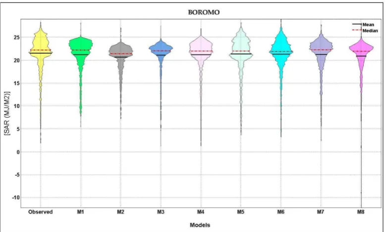
The prediction of global solar radiation can provide a reliable predictive tool to predict potentially available solar energy resources, with models developed using various climate-based input variables at specific locations, especially when there is lack of measurement equipment. In this study, a new self-tuning evolutionary predictive model called SaE-ELM was adopted to predict daily solar radiation using different input attributes (eight input combinations) based on multiple climate variables for four meteorological stations distributed over the Burkina Faso region. The performance of different models is assessed using statistical indices, regression, boxplot and Violin plots during the testing phase. The results of the current research are summarized as follows:

• The integration of the evolutionary algorithm with the self-tuning extreme learning machine model provided a reliable and robust intelligence model for global solar radiation in the Burkina Faso region, West Africa.

• The modeling results revealed that the best modeling accuracy was obtained for three stations (i.e., Bormo, Gaoua, and Po) using the fifth input combination by incorporating (WS, Tmax, Tmin,

Hmin, VPD and Eo) climate variables.

• On the other hand, the Dori station was able to demonstrate best result accuracy using WS, Tmax,

Hmax, Hmin, VPD, and Eoas input variables (M6). This was mostly owing to the influence of the

climate of the neighbouring area.

Author Contributions:Conceptualization, Z.Y.; Data curation, Z.Y.; Formal analysis, Z.Y.; Funding acquisition, Z.Y.; Investigation, Z.Y.; Resources, Z.Y.; Software, I.E.; Supervision, N.A.-A.; Validation, Z.Y.; Visualization, Z.Y.; Writing—Original draft, H.T., H.S. and Z.Y.; Writing—Review & editing, H.B., C.V., R.D. and Z.Y.

Acknowledgments:The authors would like to show their gratitude and appreciation to The National Agency of Meteorology—Burkina Faso for providing the climatological data.

Conflicts of Interest:The authors declare no conflict of interest.

Nomenclature

Self-adaptive evolutionary extreme learning machine (SaE-ELM), maximum air temperature (Tmax),

minimum air temperature (Tmin), maximum humidity (Hmax), minimum humidity (Hmin), wind speed (WS),

evaporation (Eo), vapor pressure deficits (VPD), root mean square error (RMSE), mean absolute error (MAE),

Adaptive neuro fuzzy inference system (ANFIS), Nonhydrostatic Meso-Scale Modelling (NMM), Response Surface Method (RSM).

References

1. Qazi, A.; Fayaz, H.; Wadi, A.; Raj, R.G.; Rahim, N.A.; Khan, W.A. The artificial neural network for solar radiation prediction and designing solar systems: A systematic literature review.J. Clean. Prod.2015,104, 1–12. [CrossRef]

2. Ghimire, S.; Deo, R.C.; Downs, N.J.; Raj, N. Global solar radiation prediction by ANN integrated with European Centre for medium range weather forecast fields in solar rich cities of queensland Australia.

J. Clean. Prod.2019,216, 288–310. [CrossRef]

3. Martin, C.L.; Goswami, D.Y.Solar Energy Pocket Reference; Routledge: Abingdon, UK, 2019; ISBN 1317705343. 4. Saadi, N.; Miketa, A.; Howells, M. African Clean Energy Corridor: Regional integration to promote renewable

energy fueled growth.Energy Res. Soc. Sci.2015,5, 130–132. [CrossRef]

5. Bou-Rabee, M.; Sulaiman, S.A.; Saleh, M.S.; Marafi, S. Using artificial neural networks to estimate solar radiation in Kuwait.Renew. Sustain. Energy Rev.2017,72, 434–438. [CrossRef]

6. Samuel Chukwujindu, N. A comprehensive review of empirical models for estimating global solar radiation in Africa.Renew. Sustain. Energy Rev.2017,78, 955–995. [CrossRef]

7. ¸Sen, Z. Fuzzy algorithm for estimation of solar irradiation from sunshine duration. Sol. Energy1998,63, 39–49.

8. Hou, M.; Zhang, T.; Weng, F.; Ali, M.; Al-Ansari, N.; Yaseen, Z. Global Solar Radiation Prediction Using Hybrid Online Sequential Extreme Learning Machine Model.Energies2018,11, 3415.

9. Qing, X.; Niu, Y. Hourly day-ahead solar irradiance prediction using weather forecasts by LSTM.Energy 2018,148, 461–468. [CrossRef]

10. Zhu, R.; Guo, W.; Gong, X. Short-Term Photovoltaic Power Output Prediction Based on k-Fold Cross-Validation and an Ensemble Model.Energies2019,12, 1220. [CrossRef]

11. Han, S.; Qiao, Y.; Yan, J.; Liu, Y.; Li, L.; Wang, Z. Mid-to-long term wind and photovoltaic power generation prediction based on copula function and long short term memory network.Appl. Energy2019,239, 181–191. [CrossRef]

12. De Freitas Viscondi, G.; Alves-Souza, S.N. A Systematic Literature Review on big data for solar photovoltaic electricity generation forecasting.Sustain. Energy Technol. Assess.2019,31, 54–63. [CrossRef]

13. Zou, L.; Wang, L.; Li, J.; Lu, Y.; Gong, W.; Ying, N. Global surface solar radiation and photovoltaic power from Coupled Model Intercomparison Project Phase 5 climate models.J. Clean. Prod.2019. [CrossRef] 14. Azoumah, Y.; Ramdé, E.W.; Tapsoba, G.; Thiam, S. Siting guidelines for concentrating solar power plants in

the Sahel: Case study of Burkina Faso.Sol. Energy2010,84, 1545–1553. [CrossRef]

15. David, M.; Lauret, P. Solar Radiation Probabilistic Forecasting. In Wind Field and Solar Radiation Characterization and Forecasting A Numerical Approach for Complex Terrain; Springer: Berlin/Heidelberg, Germany, 2018; pp. 201–227.

16. Fabbri, K.; Canuti, G.; Ugolini, A. A methodology to evaluate outdoor microclimate of the archaeological site and vegetation role: A case study of the Roman Villa in Russi (Italy).Sustain. Cities Soc.2017,35, 107–133. [CrossRef]

17. Zhang, J.; Zhao, L.; Deng, S.; Xu, W.; Zhang, Y. A critical review of the models used to estimate solar radiation.

Renew. Sustain. Energy Rev.2017,70, 314–329. [CrossRef]

18. Yadav, A.K.; Chandel, S.S. Solar radiation prediction using Artificial Neural Network techniques: A review.

Renew. Sustain. Energy Rev.2014,33, 772–781. [CrossRef]

19. Chen, C.; Duan, S.; Cai, T.; Liu, B. Online 24-h solar power forecasting based on weather type classification using artificial neural network.Sol. Energy2011,85, 2856–2870. [CrossRef]

20. Izgi, E.; Öztopal, A.; Yerli, B.; Kaymak, M.K.; ¸Sahin, A.D. Short-mid-term solar power prediction by using artificial neural networks.Sol. Energy2012,86, 725–733. [CrossRef]

22. Olatomiwa, L.; Mekhilef, S.; Shamshirband, S.; Petkovi´c, D. Adaptive neuro-fuzzy approach for solar radiation prediction in Nigeria.Renew. Sustain. Energy Rev.2015,51, 1784–1791. [CrossRef]

23. Wang, L.; Kisi, O.; Zounemat-Kermani, M.; Zhu, Z.; Gong, W.; Niu, Z.; Liu, H.; Liu, Z. Prediction of solar radiation in China using different adaptive neuro-fuzzy methods and M5 model tree.Int. J. Climatol.2017,

37, 1141–1155. [CrossRef]

24. Jovi´c, S.; Aniˇci´c, O.; Marseni´c, M.; Nedi´c, B. Solar radiation analyzing by neuro-fuzzy approach.Energy Build. 2016,129, 261–263. [CrossRef]

25. Landeras, G.; López, J.J.; Kisi, O.; Shiri, J. Comparison of Gene Expression Programming with neuro-fuzzy and neural network computing techniques in estimating daily incoming solar radiation in the Basque Country (Northern Spain).Energy Convers. Manag.2012,62, 1–3. [CrossRef]

26. Shavandi, H.; Saeedi Ramyani, S. A linear genetic programming approach for the prediction of solar global radiation.Neural Comput. Appl.2013,23, 1197–1204. [CrossRef]

27. Sharifi, S.S.; Rezaverdinejad, V.; Nourani, V. Estimation of daily global solar radiation using wavelet regression, ANN, GEP and empirical models: A comparative study of selected temperature-based approaches.J. Atmos. Solar-Terrestrial Phys.2016,149, 131–145. [CrossRef]

28. Ramli, M.A.M.; Twaha, S.; Al-Turki, Y.A. Investigating the performance of support vector machine and artificial neural networks in predicting solar radiation on a tilted surface: Saudi Arabia case study.

Energy Convers. Manag.2015,105, 442–452. [CrossRef]

29. Meenal, R.; Selvakumar, A.I. Assessment of SVM, empirical and ANN based solar radiation prediction models with most influencing input parameters.Renew. Energy2018,121, 324–343. [CrossRef]

30. Olatomiwa, L.; Mekhilef, S.; Shamshirband, S.; Mohammadi, K.; Petkovi´c, D.; Sudheer, C. A support vector machine-firefly algorithm-based model for global solar radiation prediction.Sol. Energy2015,115, 632–644. [CrossRef]

31. Mohammadi, K.; Shamshirband, S.; Tong, C.W.; Arif, M.; Petkovi´c, D.; Sudheer, C. A new hybrid support vector machine-wavelet transform approach for estimation of horizontal global solar radiation.

Energy Convers. Manag.2015,92, 162–171. [CrossRef]

32. Deo, R.C.; Wen, X.; Qi, F. A wavelet-coupled support vector machine model for forecasting global incident solar radiation using limited meteorological dataset.Appl. Energy2016,168, 568–593. [CrossRef]

33. Wang, J.; Xie, Y.; Zhu, C.; Xu, X. Solar radiation prediction based on phase space reconstruction of wavelet neural network.Procedia Eng.2011,15, 4603–4607. [CrossRef]

34. Amasyali, K.; El-Gohary, N.M. A review of data-driven building energy consumption prediction studies.

Renew. Sustain. Energy Rev.2018,81, 1192–1205. [CrossRef]

35. Mohanty, S.; Patra, P.K.; Sahoo, S.S. Prediction and application of solar radiation with soft computing over traditional and conventional approach—A comprehensive review. Renew. Sustain. Energy Rev. 2016,56, 778–796. [CrossRef]

36. Aybar-Ruiz, A.; Jiménez-Fernández, S.; Cornejo-Bueno, L.; Casanova-Mateo, C.; Sanz-Justo, J.; Salvador-González, P.; Salcedo-Sanz, S. A novel Grouping Genetic Algorithm-Extreme Learning Machine approach for global solar radiation prediction from numerical weather models inputs.Sol. Energy2016,132, 129–142. [CrossRef]

37. Wu, Y.; Wang, J. A novel hybrid model based on artificial neural networks for solar radiation prediction.

Renew. Energy2016,89, 268–284. [CrossRef]

38. Zhang, N.; Behera, P.K. Solar Radiation Prediction based on Recurrent Neural Networks trained by Levenberg-Marquardt Backpropagation Learning Algorithm. In Proceedings of the 2012 IEEE PES Innovative Smart Grid Technologies (ISGT), Washington, DC, USA, 16–20 Janauary 2012.

39. Ghimire, S.; Deo, R.C.; Downs, N.J.; Raj, N. Self-adaptive differential evolutionary extreme learning machines for long-term solar radiation prediction with remotely-sensed MODIS satellite and Reanalysis atmospheric products in solar-rich cities.Remote Sens. Environ.2018,212, 176–198. [CrossRef]

40. Rabehi, A.; Guermoui, M.; Lalmi, D. Hybrid models for global solar radiation prediction: A case study.Int. J. Ambient Energy2018,0, 1–10. [CrossRef]

42. Zang, H.; Cheng, L.; Ding, T.; Cheung, K.W.; Wang, M.; Wei, Z.; Sun, G. Estimation and validation of daily global solar radiation by day of the year-based models for different climates in China.Renew. Energy2019,

135, 984–1003. [CrossRef]

43. Shamshirband, S.; Mohammadi, K.; Tong, C.W.; Petkovi´c, D.; Porcu, E.; Mostafaeipour, A.; Ch, S.; Sedaghat, A. Application of extreme learning machine for estimation of wind speed distribution.Clim. Dyn.2016,46, 1893–1907. [CrossRef]

44. Glezakos, T.J.; Tsiligiridis, T. a.; Iliadis, L.S.; Yialouris, C.P.; Maris, F.P.; Ferentinos, K.P. Feature extraction for time-series data: An artificial neural network evolutionary training model for the management of mountainous watersheds.Neurocomputing2009,73, 49–59. [CrossRef]

45. Salcedo-Sanz, S.; Deo, R.C.; Cornejo-Bueno, L.; Camacho-Gómez, C.; Ghimire, S. An efficient neuro-evolutionary hybrid modelling mechanism for the estimation of daily global solar radiation in the Sunshine State of Australia.Appl. Energy2018,209, 79–94. [CrossRef]

46. Ebtehaj, I.; Sattar, A.M.A.; Bonakdari, H.; Zaji, A.H. Prediction of scour depth around bridge piers using self-adaptive extreme learning machine.J. Hydroinformatics2017,19, 207–224. [CrossRef]

47. Dash, R.; Dash, P.K.; Bisoi, R. A self adaptive differential harmony search based optimized extreme learning machine for financial time series prediction.Swarm Evol. Comput.2014,19, 25–42. [CrossRef]

48. Price, K.V. Differential Evolution. InIntelligent Systems Reference Library; Springer: Berlin/Heidelberg, Germany, 2013.

49. Huang, G.-B.; Zhu, Q.-Y.; Siew, C.-K. Extreme learning machine: Theory and applications.Neurocomputing 2006,70, 489–501. [CrossRef]

50. Huang, G.B.; Chen, L. Convex incremental extreme learning machine.Neurocomputing2007,70, 3056–3062. [CrossRef]

51. Huang, G.-B.; Zhou, H.; Ding, X.; Zhang, R. Extreme learning machine for regression and multiclass classification.IEEE Trans. Syst. Man. Cybern. B Cybern.2012,42, 513–529. [CrossRef]

52. Yaseen, Z.M.; Deo, R.C.; Ebtehaj, I.; Bonakdari, H. Hybrid Data Intelligent Models and Applications for Water Level Prediction. InHandbook of Research on Predictive Modeling and Optimization Methods in Science and Engineering; IGI Global: Hershey, PA, USA, 2018.

53. Al Sudani, Z.A.; Salih, S.Q.; Yaseen, Z.M. Development of Multivariate Adaptive Regression Spline Integrated with Differential Evolution Model for Streamflow Simulation.J. Hydrol.2019,573, 1–12. [CrossRef] 54. REN21.Renewables 2017: Global Status Report; REN21: Paris, France, 2017; Volume 72, ISBN 978-3-9818107-0-7. 55. Tao, H.; Diop, L.; Bodian, A.; Djaman, K.; Ndiaye, P.M.; Yaseen, Z.M. Reference evapotranspiration prediction

using hybridized fuzzy model with firefly algorithm: Regional case study in Burkina Faso.Agric. Water Manag.2018,208, 140–151. [CrossRef]

56. Legates, D.R.; Mccabe, G.J. Evaluating the use of “goodness-of-fit” measures in hydrologic and hydroclimatic model validation.Water Resour. Res.1999,35, 233–241. [CrossRef]

57. Moriasi, D.N.; Arnold, J.G.; Van Liew, M.W.; Binger, R.L.; Harmel, R.D.; Veith, T.L. Model evaluation guidelines for systematic quantification of accuracy in watershed simulations.Trans. ASABE2007,50, 885–900. [CrossRef] 58. Benali, L.; Notton, G.; Fouilloy, A.; Voyant, C.; Dizene, R. Solar radiation forecasting using artificial neural network and random forest methods: Application to normal beam, horizontal diffuse and global components.

Renew. Energy2019,132, 871–884. [CrossRef]

59. Keshtegar, B.; Mert, C.; Kisi, O. Comparison of four heuristic regression techniques in solar radiation modeling: Kriging method vs RSM, MARS and M5 model tree.Renew. Sustain. Energy Rev.2018,81, 330–341. [CrossRef]

60. Kisi, O.; Heddam, S.; Yaseen, Z.M. The implementation of univariable scheme-based air temperature for solar radiation prediction: New development of dynamic evolving neural-fuzzy inference system model.

Appl. Energy2019,241, 184–195. [CrossRef]

61. Prasad, R.; Ali, M.; Kwan, P.; Khan, H. Designing a multi-stage multivariate empirical mode decomposition coupled with ant colony optimization and random forest model to forecast monthly solar radiation.

Appl. Energy2019,236, 778–792. [CrossRef]