A philosophy for the development of kinetic models in predictive microbiology

A Philosophy for the Development of Kinetic Models

in

Predictive Microbiology

Thomas Ross B.Sc.(Hons.)

submitted

in

fulfilment of the requirements for the degree of

Doctor of Philosophy

University of Tasmania

Hobart

DECLARATION

I declare that this thesis contains no material which has been accepted for the award of any other degree or diploma in any tertiary institution and; to the best of my knowledge and belief, contains no material previously published or written by another person, except where due reference is made in the text of the thesis.

)

J;A

~,Ross

I

/1993

This thesis may be made available for loan and limited copying in accordance with

the Copyright Act 1968. ~·/

iii

ABSTRACT

The development of predictive microbiology is reviewed and specific limitations relating to the generation of kinetic models identified. The issues of variability of

response, lag time response, fluctuating environments and their effects, microbial interactions, choice of model for describing bacterial growth curves, and mechanistic

versus empirical models are discussed and exemplified using experimental data. A

philosophy for the development of reliable predictive kinetic models is developed

and the appropriateness of that philosophy examined by simulations and reference to

novel and independently published experimental data.

Specifically, the use of turbidimetric techniques is advocated for primary model

development, methods of calibration to traditional (i.e. viable count) methods demonstrated, and the reliability of that calibration demonstrated. Using that methodology, models for the growth of several strains of Staphylococcus aureus

and Listeria monocytogenes are generated. Novel indices of the reliability of models

are developed, and used to assess the S. aureus 3b and the L. monocytogenes models,

for constant environmental conditions, by comparison to published and novel data.

An assessment of the three~parameter (temperature, water activity, pH) square-root

modelt is made using data for the growth of L. monocytogenes. A deliberately

minimal experimental design was used to 'test to destruction' the proposed methodology, and revealed potential shortcomings of the lack of replication.

It is concluded that the experimental strategy proposed offers an efficient method for

generating the quantity of data required for the development of reliable kinetic

models from which to predict the growth of spoilage and pathogenic organisms of

relevance to foods.

Technologies for the transfer of validated, laboratory-generated models to the food

industry are demonstrated, and a mechanistic interpretation of the basis of the

empirical square-root relationship developed.

t McMeekin, T.A., Ross, T. and Olley, J. 1992. Application of predictive microbiology to assure the quality and safety of fish and fish products. Int. J. Food Microbial. 15: 13-32.

ACKNOWLEDGMENTS

I would like to acknowledge sincerely the contributions of:

my academic supervisors, Prof. T. A. McMeekin and Dr. J. Olley, for providing limitless support, stimulus, crisis intervention, and for providing the environment and opportunity;

The Rural Industries Research and Development Corporation for generous and gracious financial support;

David Ratkowsky for statistics and nonlinear regression expertise;

Dr. Kevin Sanderson, and Mr. Simon James for setting up and maintaining the computer facilities;

Glen McPherson for preparation of the Gompertz function fitting programme; Dr. Fred Grau for Listeria cultures and coilaboration;

Dr. Charles Jason and Dr. Peter Franzmann for insightful questions and comments; all of my student colleagues, and staff of the Department of Agricultural Science

(particularly Sally and Bill), for the help, good times, good ideas and just for being there;

CONTENTS

ABSTRACT ACKNOWLEDGMENTS CONTENTS ABBREVIATIONS PUBLICATIONS 1

1.1

1.1.1

1.1.2

1.1.3

1.1.4

1.1.4.1

1.1.4.2

1.1.5

1.1.6

1.1.7

1.2

1.3

2

2.1

2.1.1

2.2

2.2.1

2.2.2

2.2.3

2.2.4

2.2.5

2.2.6 2.2.7

2.2.8

2.2.9

2.3

2.3.1

2.3.2

2.3.3

2.3.4

2.4

2.4.1

2.4.2

2.5

2.5.1

2.5.2

2.5.3

2.5.4

2.5.5

INTRODUCTION LITERATURE REVIEW History

Approaches and Potential Benefits Definitions and Rules for Modelling Models

Kinetic models Probability models

Potential Problems and Solutions Technology

Summary

CONTEMPORARY RESEARCH OBJECTIVE OF THIS THESIS

KINETIC MODEL GENERATION: HYPOTHESES INTRODUCTION

Empirical vs Mechanistic Models PLANNING

Independent Variables Interactions

Range of Values

Preparation of Inocula Inoculum Size

Mixtures of Strains and Species Response Variable

Experimental Model Quantity of Data

MATHEMATICAL DESCRIPTION Introduction

The Principle of Least Squares Stochastic Behaviour

Regression Analysis

VALIDATION AND MAINTENANCE Validation Techniques

Laboratory to Field

RATIONALISATION OF EXPERIMENTAL PROTOCOL Response Variable

Axenic or Mixed Culture? Evaluation by Simulation Response Surface Design

3

PRIMARY MODELLING

3.1

SELECTION OF A SIGMOID FUNCTION TO DESCRIBE THE RESPONSE

3.1.1 .

Introduction

3.1.2

Theory

3.1.2.1

Modified-Gompertz function

3.1.2.2

The Dalgaard (1993) modification of the logistic function

3.1.3

Methods

3.1.4

Results

3.1.5.

Discussion

3.2

DEVELOPMENT OF A TURBIDIMETRIC METHOD

FOR DOUBLING TIME DETERMINATION

3.2.1

Introduction

3.2.2

Theory

3.2.3

Methods and Materials

3.2.3.1

Relationship between change in %transmittance and population density

3.2.3.2

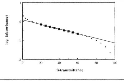
Deviation from Beer's Law

3.2.3.3

Relationship between wavelength and generation time estimate

3.2.3.4

Evaluation of Eqn. 3.13

3.2.4

Results

3.2.5

Discussion

3.3

COMPARISON OF TURBIDIMETRIC AND VIABLE COUNT

METHODS FOR GENERATION TIME ESTIMATION

3.3.1

Introduction

3.3.2

Methods and Materials

3.3.3

Results

3.3.4

Discussion

3.4

CONCLUSIONS

4 SECONDARY MODELLING

4.1

4.1.1

4.1.2

4.1.3

4.2

4.2.1

4.2.2

4.2.2.1

4.2.2.2

4.2.2.3

4.2.2.4

4.2.2.5

4.3

4.3.1

4.3.1.1

4.3.1.2

4.3.2

4.3.3

4.3.4

4.3.4.1

4.3.4.2

4.3.4.3

INTRODUCTION Staphylococcus aureus Listeria monocytogenes Existing Predictive Models MATERIALS AND METHODS

Materials Methods

Inoculation procedures Growth rate estimation Parameter estimation

Environmental history effects Model generation

RESULTS

Parameter Estimation by 'Iterative' Methods

T min estimates

awmin estimates

pH Response

Environmental History Effects Model Construction

Stochastic considerations

Staphylococcus aureus 3b

4

SECONDARY MODELLING (cont.) 4.4 4.4.1 4.4.1.1 4.4.1.2. 4.4.1.3 4.4.2 4.4.3 4.4.4 4.4.4.1 4.4.4.2 4.4.4.3 4.4.5 DISCUSSION

Responses to Individual Constraints Temperature and water activity Derived estimates

pH response

Environmental History Effects Strain to Strain Variability Evaluation of Hypotheses

Independence of effects Iterative approach Experimental design Summary

5

MODEL EVALUATION

93 95 95 95 99 101 101 101 102 102 103 104

5.1 INTRODUCTION 105

5.2 MATERIALS AND METHODS 106

5.2.1 Materials 106

5.2.2 Data Sources and Bases of Comparison 106

5.2.2.1 Data sources 106

5.2.2.2 Indices of bias and precision 107

5.2.3 Growth Rate Determinations in Foods 107

5.2.3.1 Preparation of inoculum 107

5.2.3.2 Product inoculation 108

5.2.3.3 Incubation of inoculated product 108

5.2.3.4 Assessment of growth 108

5.2.3.5 Growth rate estimation 109

5.2.3.6 Growth on prawns 109

5.2.3.7 Growth on smoked Atlantic salmon 109

5.2.3.8 Growth on re-brined smoked salmon 110

5.2.3.9 Growth in milk 110

5.2.3.10 Water activity determinations 110

5.3 RESULTS 110

5.4 DISCUSSION 124

5.4.1 Models for S. aureus 3b 125

5.4.2 Models for L. monocytogenes Murray B 126

5.4.3 Models for L. monocytogenes Scott A 127

5.4.4 Extrapolation 128

5.4.5 Conclusions 130

6

TERTIARY MODELS: TEMPERATURE FUNCTION

INTEGRATION

6.1 INTRODUCTION 132

6.2 INTEGRATION 132

6.2.1 Temperature Function Integration and Food 133 6.2.2 Temperature Function Integration Devices 135

6.2.3 A Manual Tertiary Model 135

6.2.4 A Spreadsheet-based Tertiary Model 137

6.2.4.1 Input 138

6.2.4.2 Processing 138

6.2.4.3 Output 141

6.2.4.2 User interface 142

6.3.2.5 Further developments 142

7

MECHANISMS FOR THE MICROBIAL GROWTH RATE RESPONSE TO TEMPERATURE

7.1 INTRODUCTION 150

7.2 MODEL DEVELOPMENT 150

7.2.1 Starting Assumptions 150

7.2.2 Model Derivation 152

7.3 METHODS 155

7.4 RESULTS 156

7.4.1 Analysis of the Model 156

7 .4.2 Enzyme Catalysis Data 157

7.4.3 Growth Curves: Simulated Data 158

7.4.4 Growth Curves: Experimental Data 161

7.5 DISCUSSION 161

7.5.1 AP Data 161

7.5.2 Microbial Growth Rate Data 166

7.5.3 Critique of Model Bases 166

7.5.4 Conclusions 168

8 SUMMARY AND CONCLUSIONS 170

REFERENCES 172

APPENDICES 198

A1 DATA SETS USED IN 3.1, AND SUMMARY 198

A2 COMMON METHODS AND MATERIALS 201

A2.1 Materials 201

A2.1.1 Reagents 201

A2.1.2 Organisms 201

A2.1.3 Culture Media and Reagents 202

A2.1.4 Equipment 203

A2.2 Methods 204

A3 DATA SETS USED FOR MODEL GENERATION 206

A4 GIBBS FREE ENERGY OF PROTEIN DENATURATION AS

ABS ABSctn Absobs aw BHIB/A BPA CFU !l.Gden k* MAFF MPD OLSA PCA pHi pHr pH mid

!l.pH RMS RSS RH rsd SD SE

tc

tcmin

IG%T

tcvc

T TGI TSB/A 6.%T !l.%T3o %T f.l max* USDA

vc

ABBREVIATIONS USED IN THIS THESIS

'true' absorbance of a sample after correction, if necessary, for high concentration deviation

absorbance of a diluted sample

observed absorbance (undiluted sample) water activity

brain heart infusion broth/agar Baird-Parker Agar

colony forming unit

Gibbs free energy change associated with protein denaturation reciprocal of response time

Ministry of Agriculture Food and Fisheries (UK)

maximum population density (of a bacterial culture in a given environment)

Oxford Listeria Selective Agar Plate Count Agar

initial pH (of a broth culture) final pH (of a broth culture) midpoint of pHi and pHr

change in pH of culture medium

mean of the sum of the squares of residuals residual sum of squares

relative humidity("" 100 x aw)

relative standard deviation standard deviation

staphylococcal enterotoxin

mean generation time (of a bacterial population)

minimum observed generation time (of a bacterial population during )

tGmin estimate derived from %transmittance data

tGmin estimate derived from viable count data

temperature

temperature gradient incubator tryptone soy broth/agar

change in %transmittance of a bacterial culture since inoculation

time required for %T of a culture to change by 30% from that at the t

=

0 % transmittance

maximum specific growth rate of a bacterial culture United States Department of Agriculture

viable count

* In the predictive microbiology literature, the symbol k has often been used to denote the reciprocal of microbial response times and, thus, to denote microbial growth rate. The designation of k as the 'growth rate constant'. or specific growth rate, is a more established usage. The relationship between the generation time, GT, and specific growth rate is:

specific growth rate

=

Ioge2/GT

0.693/GT

PUBLICATIONS

REFEREED PAPERS.

Ross, T. (1987). Belehnidek Temperature Functions and Growth of Microorganisms. CSIRO-DSIR Joint Workshop on Seafood Processing, Nelson, New Zealand,

Apri/1986. CSIRO Tasmanian Regional Laboratory Occasional Paper No. 18.

Ross, T. and McMeekin, T.A. (1991) Predictive Microbiology. Applications of a square root model. Food Australia, 43: 202-207.

McMeekin, T.A. and Ross, T (1991). Potential of predictive microbiology to improve the microbiological safety and shelf life of poultry meat products. pp: 109-116 in RWAW Mulder and AW de Vries (Eds.). Quality of Poultry Products

III. Safety and Marketing Aspects. Spelderholt Centre for Poultry Research and

Information Services. Beekbergen, The Netherlands.

Ratkowsky, D.A., Ross, T., McMeekin, T.A. and Olley, J. (1991). Comparison of Arrhenius-type and Belehnidek-type models to predict bacterial growth in foods.

Journal of Applied Bacteriology, 15: 13-32.

McMeekin, T.A., Ross, T. and Olley, J. (1992). Application of predictive food microbiology to improve the safety and quality of fish and fisheries products.

International Journal of Food Microbiology, 71: 452- 459.

Ross, T. (1993). Belehradek-type models. Journal of Industrial Microbiology, 12: 180- 189.

McMeekin, T.A. and Ross, T. (1993). Use of predictive microbiology in relation to meat and meat products. pp: 257 - 274 in Proceedings of the 39th International

Congress of Meat Science and Technology, Calgary, August 1993.

McMeekin, T.A. and Ross, T. (1993). Development of predictive microbiology for food industry applications. 3rd Singapore Society for Microbiology International

Congress, Singapore, December, 1993.

Ross, T. and McMeekin, T.A. (in press). Predictive microbiology - a review. International Journal of Food Microbiology.

Dalgaard, P., Ross, T., Kamperman, L., Neumeyer, K. and McMeekin, T.A. (in

press). Estimation of bacterial growth rates from turbidimetric and viable count

data. International Journal of Food Microbiology.

MONOGRAPHS

McMeekin. T.A., Olley, J., Ross, T. and Ratkowsky, D.A. (1993). Predictive

u ....

the growth of bacterial cultures, despite the immense

complexity of the phenomena to which it testifies, generally

obeys relatively simple laws ... The accuracy, the ease, the

reproducibility of bacterial growth constant determinations is

remarkable and probably unparalleled, so far as biological

quantitative characteristics are concerned."

INTRODUCTION

In 1983, at a Symposium of the Society for Applied Bacteriology, a panel of 30 expert food microbiologists using the Delphi technique of intuitive forecasting (Dalkey, 1967) predicted that the assessment of shelf life by computers, drawing on databases for the growth of spoilage organisms, had an 80% probability of being widely used by 1993. Nonetheless, at least 25% of the panel considered it improbable that such an approach would be accepted even at the beginning of the 21st century (Jarvis, 1983).

In 1992, the UK Ministry of Agriculture, Fisheries and Food launched 'Food Micromodel' - a food microbiology advisory service based on a database and mathematical models describing the growth response to environmental factors of food-borne pathogens. This service is a realisation of that earlier prophecy, and part of a new approach to the assurance of the microbiological quality and safety of food currently known as "Predictive Microbiology".

Predictive microbiology is based upon the premise that the responses of populations of microorganisms to environmental factors are reproducible, and that by considering environments in terms of identifiable dominating constraints it is possible, from past observations, to predict the responses of those microorganisms. In general, a reductionist approach is adopted and microbial responses are measured under defined and controlled conditions. The results are summarised in the form of mathematical equations which, by interpolation, can predict responses to novel sets of conditions, i.e. those which were not actually tested. Proponents claim that such an approach will enable:

i) prediction of the consequences, for product shelf life and safety, of changes to product formulation

ii) objective evaluation of processing operations and, from this, an empowering of the HACCP approach

iii) objective evaluation of the consequences of lapses in process and storage control

iv) the rational design of new processes and products, to achieve required levels of safety and shelf life.

countries acting collaboratively to examine growth responses of spoilage and pathogenic organisms in a wide range of natural products. In the United States of America predictive microbiology research is centred at the Microbial Food Safety Research Unit of the USDA in Pennsylvania, which has resulted in the preparation and release of software called the 'Pathogen Modeling Program'.

Earlier reviews of the subject include Farber (1986), McMeekin and Olley (1986), Baird-Parker and Kilsby (1987), Gibson and Roberts (1989), Gould (1989), Roberts (1989, 1990), Gibbs and Williams, (1990), Buchanan (1991a), and Baker and Genigeorgis (1993). A monograph on the subject has been prepared by McMeekin et al. (1993).

1.1 LITERATURE REVIEW

1.1.1 History

The use of mathematical models in food microbiology is not new. Baird-Parker and Kilsby (1987) point out that models for the thermal destruction of microorganisms by heat are well established in the literature and industry, e.g. the 'botulinum cook' (see Stumbo et al., 1983). Mathematical modelling is also well developed in the fermentation industry. The application of mathematical modelling techniques to the

growth and survival of microorganisms in foods, however, did not receive wide

attention until the 1980's. McMeekin et al. (1993) suggest that two related trends contributed to the increased willingness to consider predictive modelling. The first was the marked increase in the incidence of major food poisoning outbreaks during the 1980's, which led to an acutely increased public awareness of the requirement for a safe and wholesome food supply. The second was the realisation by many food microbiologists, and clearly identified by Roberts and Jarvis (1983), that traditional microbiological methods to determine quality and safety were limited by the time needed to obtain results, and that the more rapid, indirect methods did not give a response until very large numbers of cells were present, i.e. they had little predictive value. Buchanan ( 1991 b) points to another factor in the realisation of the concept: that of increased ready access to computing power.

3

temperature of many spoilage processes, and also of bacterial growth, and in Daud et

al. (1978) was able to apply the general spoilage model (Olley and Ratkowsky, 1973a)

to the spoilage of chicken.

A second area of research dealt with the prevention of botulism, and other microbial intoxications. Genigeorgis' group at the University of California sought to go beyond the work of other researchers (e.g. Baird-Parker and Freame, 1967) on defining combinations of factors that would prevent pathogen growth and toxin formation. Their approach was to model the 'log reduction' of bacterial numbers due to intrinsic and extrinsic properties of foods, such as temperature, pH, N aCl concentration, etc. described as 'hurdles' by Leistner and Rodel (1976). The log reduction was then related to the probability of bacterial growth or toxin production (Genigeorgis et al., 1971a).

At about the same time workers at the UK Ministry of Agriculture Fisheries and Food, were also involved in describing growth-controlling combinations of factors (Roberts and Ingram, 1973; Bean and Roberts, 1974), but did not begin to summarise their results as equations describing the probability of growth or toxin production until several years later (Jarvis et al., 1979; Roberts et al., 1981 a,b,c). Similarly, in the Netherlands, Kreyger (1972) had used a modelling approach to predict the mould-free storage life of cereals during ocean transport but presented results as diagrams only.

During the 1980's increased attention was given to modelling the growth of microorganisms of concern, with a number of groups publishing in this area. Genigeorgis' approach was applied to growth rate modelling (Metaxapoulos et al.,

1981a, b). Ratkowsky et al. (1982) and Ratkowsky et al. (1983) contributed simple

and apparently universal models relating the growth rate of bacteria to temperature. Broughall et al. (1983) introduced a model relating the growth rate of bacteria to

temperature and water activity which was built upon by Broughall and Brown (1984) to include the effect of pH also. Roberts group began growth rate modelling in 1987 (Gibson et al., 1987). Their efforts led ultimately to an entirely different approach

which has become the basis of programmes which resulted in Food Micromodel and the Pathogen Modeling Program.

predictions of quality and safety to be made speedily with considerable financial benefit". This succinct statement of the need for such an approach places into perspective the vision of Scott (1937) who wrote: "A knowledge of the rates of growth of certain microorganisms at different temperatures is essential to the studies of the spoilage of chilled beef. Having these data it should be possible to predict the relative influence on spoilage exerted by various microorganisms at each storage temperature. Further it would be feasible to predict the possible extent of changes in populations during the initial cooling of sides of beef in the meatworks when the meat surfaces are frequently at temperatures very favourable to microbial proliferation".

1.1. 2 Approaches and Potential Benefits

Predictive microbiology has to date usually been considered under two main headings. These are kinetic models, that is, modelling the extent and rate of growth of microorganisms of concern, and probability modelling: the construction of models to predict the likelihood of some event, such as a spore germinating or a detectable amount of toxin being foimed, within a given time period .

The hypothesis underlying the kinetic modelling approach is that many perishable foods represent a 'pristine' environment open to exploitation by microorganisms, and that the growth of bacteria in this environment approximates a 'batch culture'. Typically, nutrients will not limit growth until spoilage has occurred or infectious dose levels are exceeded and, consequently, factors such as temperature, pH, water availability, gaseous atmosphere, preservatives etc. dictate the rate and extent of microbial proliferation. Thus, a detailed knowledge of the growth responses of microorganisms to those environmental factors should enable prediction of the extent of microbial proliferation in foods during processing, distribution and storage by monitoring the environment presented to the organism by the food during those

operations. In the area of kinetic modelling two distinct approaches can also be identified. In one, growth rate is modelled and then used to make predictions in accordance with exponential population growth. This approach has been used by a number of groups (Broughall et al., 1983; Smith, 1987; Blankenship eta!., 1988; Fu et al., 1991; Dickson eta!., 1992; McMeekin et al., 1993). In the second, a sigmoid

function is fitted to the observed population growth curve and the effect of environmental factors on the values of parameters of that fitted sigmoid curve are modelled. This approach was introduced by Gibson et al. (1988). In both approaches

In the simplest case, when developing models to predict the probability of growth of pathogens or production of toxins, replicate samples of a known inoculum are observed under defined environmental conditions for a fixed period of time. At the end of the incubation period samples are examined for the presence of toxin, or detectable growth. The probability of detectable growth/toxin production within that incubation period can be calculated from the proportion of replicates positive for growth/toxin production. As this proportion is dependent upon the specific environmental conditions, a model relating the probability to those conditions may be derived. Typically, observations are made at a number of times, and the probability of detectable growth/toxin production is observed to increase with time. To date, the primary application of probability modelling has been to describe the effect of environmental factors on spore germination.

Gould (1989) considered that predictive microbiology would "encourage a more integrated approach to food hygiene and safety which will impact on all stages of food production, from raw material acquisition and handling, through processing, storage, distribution, retailing and handling in the home". In addition to the general benefits outlined above, modelling also provides a basis for comparison of data from diverse sources on the growth of microorganisms in foods, and should result in increased productivity by reducing the need for the time consuming and invasive microbiological testing procedures currently practiced. Genigeorgis (1981) noted that 'predictive microbiology' would provide a rational basis for the drafting of guidelines, criteria and standards pertaining to the microbiological status of food, and both McMeekin and Olley (1986) and Walker and Jones (1992) have pointed to the value of predictive microbiology, and devices based upon it, as educational tools for food workers and handlers. Davey (1992a) drew attention to major difficulties faced by food process engineers due to the poor understanding of the combined influences of environmental factors on the kinetics of bacterial growth and inactivation. He welcomed predictive modelling as a solution to that problem, and predicted that such models, coupled with indirect sensors and computers, would enable 'real-time' food process optimisation through automated in-line process control.

The potential benefits of the modelling approach are numerous but all derive from better understanding, and consequently control, of the microbial ecology of foods that predictive modelling represents.

1.1.3 Definitions and Rules for Modelling

Independent, explanatory or predictor variables are those which it is believed will explain the type and magnitude of the response observed. In the case of models for food microbiology, these will typically be temperature, pH, water activity, and other agents in the modelled system which affect the rate of response of the modelled organism. Response or dependent variables are those properties of the system which are governed by the independent variables. In the case of predictive models in food microbiology, this will usually be the rate or duration of some microbial growth process or the probability of an event or condition arising within a given time.

A model is formulated to describe the known or assumed qualitative relationship between the predictor and response variables, but it is the parameters of the equation which quantify the relationship. Parameters, which are constants for a given set of experimental conditions, must be estimated from the data to give the best possible fit to the data. The usual means of estimation of parameters is the minimisation of the values of the residuals, which are the differences between the observed values of the response variable and those predicted by the fitted equation.

There is always some error inherent in any measurement of an observation. This error is the difference between the particular observation and the mean, or predicted, response. Accordingly, in any mathematical description of a data set there will also be some error between the predicted and observed values. The behaviour of the error can be investigated and described. For example it may, on average, be a constant value irrespective of the magnitude of the response. Alternatively it may be a function of the magnitude of the response. Description of this behaviour is an integral part of the modelling process and is expressed in the error, or stochastic, term of the model. The deterministic part of the model describes the relationship between the variables.

The error behaviour is particularly significant when fitting equations to data because those observations having larger error will be more influential in determining the parameter estimates when using residual minimisation techniques, e.g. least squares, for fitting. It is desirable that all observations are given equal weight in the fitting process, and for this reason one seeks to 'homogenise' the variance, i.e. to make the magnitude of the error independent of the magnitude of the observed response. Weighting may be applied to the data during the fitting process, so that those values with smaller residuals are given greater weight. An alternative is to transform the data mathematically, for example by taking the logarithm or some power of all the values, to thus homogenise the variance. The transformed data are then used in the fitting process.

y

=a+

p

x

+

y

x2

is classified as a linear regression model, since the parameters

a,

~. andy appear linearly (i.e. as the sum of individual effects), although the relationship between the response variable y and the explanatory variable x describes a curved line. In nonlinear models the parameters do not appear linearly. The important differences between these two types of model are the manner in which they are fitted to data, and their estimation properties once fitted. The best estimates of parameters of linear models have explicit (algebraic) solutions. Best estimates of nonlinear models, however, do not have explicit solutions and are typically estimated by an iterative process in which approximate values of the parameter values are used as 'starting' values. Using these values a measure of the 'goodness-of-fit' of the fitted model is made. In the next step, new parameter values are sought which increase the 'goodness-of-fit' of the model to the data. This step-wise process is continued for a predetermined number of steps or until no further improvement in goodness-of-fit can be obtained. If at this stage the 'goodness-of-fit' meets some predetermined criteria of acceptability, this condition is known as 'convergence'. Not all data sets will achieve convergence nor does achievement of convergence guarantee that those parameter values are the best possible. Although nonlinear regression software is readily available, there is an element of expertise required when fitting data to nonlinear models.

independent variable independent (explanatory) variables

y

₌

a

+

+

yXz

+

E

parameters error term

Ratkowsky (1983, 1990) has argued that it is a desirable goal of nonlinear modelling to search for models that are "close-to-linear", that is, ones that come close to achieving the properties that are attainable in linear models. 'Far-from-linear' models may have such highly biased estimators for at least one parameter that one can not have much faith that the estimates produced are sufficiently close to the true (but unknown) parameter values. Some practical considerations to which modellers should pay attention when engaged in nonlinear regression modelling are:

i) parsimony

ii) parameter estimation properties iii) range of variables

iv) stochastic assumptions v) interpretability of parameters

which are discussed in greater detail in Chapter 2 of McMeekin et al. ( 1993 ), Chapter 3 of Bates and Watts (1988) and Chapters 2 and 10 ofRatkowsky (1990).

It is intuitively apparent that a fundamental aspect of a predictive model is that it describes observed data accurately, but it is equally important that it can predict accurately responses to novel conditions. Unless a model has a proven mechanistic basis, predictions from that model should be based only on interpolation. Hence it is essential to have as full a range of the variables as possible. When reliable statistical analysis demonstrates that competing models predict equally well, other characteristics of the model such as parsimony; parameter estimation behaviour; parameter interpretability should be considered. A further, almost trivial, consideration in the selection of models is their ease of use, but it is only when all other criteria fail to provide discrimination between competing models that this be considered a basis for selection. The ease of use of a particular model will, of course, depend upon ones own environment, resources and background, and personal preferences.

Davey (1992b) suggested the adoption of 'express terminology' in predictive microbiology to clarify discussion of issues. His comments relate to the use of the terms to categorise and describe models unambiguously, and to seek a uniform usage of the terms 'interactive' in relation to environmental variables, and 'validated' in terms of the ability of models to predict responses to novel conditions, i.e. data not used to generate the model. Those comments were, in general, endorsed by Baranyi and Roberts (1992), who also suggested consistent terminology for describing rates of growth, and also by Whiting and Buchanan (1993).

1.1. 4 Models

reviewed by Ratkowsky eta/. (1991) and Heitzer et al. (1991). In this category are recognised four main model types which are:

Belehradek- or square-root-type models Arrhenius-type models

Modified Arrhenius, or 'Davey' models Polynomial, or 'Response Surface' models

There is less divergence in the form of probability models published to date, but slightly different forms have been adopted by the groups of Genigeorgis, Roberts and Lund.

1.1.4.1 Kinetic models Belehrddek-type models

Ratkowsky et al. (1982) introduced a simple model to describe the rate of microbial

growth as a function of temperature. The model was based upon the observation of Ohta and Hirahara (1977) that the square root of the rate of nucleotide degradation in carp muscle is related to temperature. Olley (1986) describes how she and her coworkers found this relationship well described the growth rate response to temperature of many bacteria. The latter model has the form:

=

b (T- T min) ( 1.1)

where k is the rate of growth, Tis the temperature, T min is a notional minimum temperature for growth and b is a coefficient to be estimated. Subsequently it was shown that the 'square root' model was a special case of the Belehnidek (1930) equation widely used in other biological sciences (Ross, 1987). Ratkowsky eta/. (1983) extended the applicability of their equation to include temperatures superoptimal for growth. This new model had the form:

=

b (T-T min)O-exp(c(T-T max))) (1.2)

where k, T, T min. and b have the same meaning as above and T max 1s a notional maximum temperature for growth analogous to T min and c is a coefficient to be estimated.

Minor modifications to this model were advocated by Zwietering eta!. (1991) and

Kohler et al. (1991). This general form was further extended by McMeekin eta!.

=

( 1.3)

where k, T , T min and b have the same meaning as above, aw is the water activity and aw min is a notional minimum water activity for growth

and by Adams et al. (1991) who incorporated a term for pH:

=

(1.4)

where k, T, T min and b have the same meaning as above and pH min is a

notional minimum pH for growth.

The success of the Equations (1.3) and (1.4) led McMeekin et al. (1992) to conjecture that the effects on microbial growth of temperature, pH and water activity might be described by a simple four parameter model of the following form:

=

(1.5)

where all parameters are as previously defined.

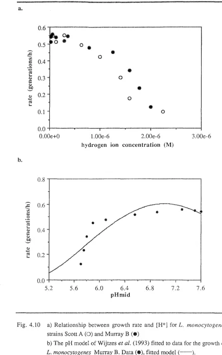
This equation, and a variation of it, introduced by Zwietering et al. (1992a), incorporating a pH term to cover the entire pH range was subsequently applied by Wijtzes et al. (1993) to describe data for the growth of Listeria monocytogenes.

Whilst Eqn. (1.1) may be expressed as a linear model, Eqns. (1.2) to (1.5) are nonlinear, and the parameters of those models must be estimated by iterative procedures.

Arrhenius-type models

The simplest form of 'Arrhenius-type' model in use in predictive microbiology is the 'classical' Arrhenius equation:

ln

k

=

I n A - -Ea

RT (1.6)

where, when applied to microbial growth, k is the rate of growth, A is a parameter to be fitted, R is the gas constant (8.314 J K-1 _{moi-l), T is}

temperature, and Ea is sometimes interpreted as the activation energy of the

growth-rate-limiting reaction or, to avoid this assumption, is simply referred to as a 'temperature characteristic'.

was inadequate to describe the rate response to temperature of complex biological systems. More sophisticated models were developed to take into account the deviation, at high and low temperatures, from the rate predicted by the simple Arrhenius equation. A number of models of essentially similar form were developed by Johnson and Lewin (1946), Hultin (1955), and Sharpe and DeMichele (1977). The latter model was reparameterised by Schoolfield et al. (1981). Of the Arrhenius-type models, the model of Schoolfield et al. (1981) has received the most attention in the predictive microbiology literature, having been used by workers at U nil ever Research in the UK (Broughall et al., 1983; Broughall and Brown, 1984; Adair et al., 1989). In its original parameterisation, this nonlinear model has the form:

P<25 )

2~8

exp{

~ (2~8- ~)}

=----~---7---~~--~---~

K 1+exp{HL

(-1

-~J}+exp{HH

( 1

-~J}

R T₁₁₂ T R T₁₁₂ T

L H

1

(1.7)

where Tis absolute temperature, R is the universal gas constant and, for modelling bacterial growth, the other parameters have been interpreted as follows: K is the response (e.g. generation) time, P(25) is a scaling factor equal to the response rate (1/K) at 25°C, HA is the activation energy of the

rate-controlling reaction, HL is the activation energy of denaturation of the

growth-rate-controlling enzyme at low temperatures, HH is the activation energy of denaturation of the growth-rate-controlling enzyme at high temperatures, TmL is the lower temperature at which half of the growth-rate-controlling enzyme is denatured, _Tm11 is the higher temperature at which half of the growth-rate-controlling enzyme is denatured.

For modelling in the suboptimal temperature region only, the model can be simplified by the deletion of terms relating to high temperature inactivation, i.e. the second exponential term in the denominator.

Broughall et al. (1983) further developed this temperature-rate model to include the effects of water activity by modelling the change in the parameters ln P(25),

H A, 1n (-HL) and TmL using expressions of the general form:

parameter= F + G(aw - 0.95)

Broughall and Brown (1984) extended this approach to include the effect of pH. The effects of pH and water activity on the fitted values of the parameters ln P(25), HA,HL

and T112L were modelled using expressions of the form:

where pHS and awS are approximations of the mid-point of the range of pH and aw respectively for which data were obtained. The resulting equation thus required the estimation of twenty parameters to describe the effect of temperature, pH and water activity on bacterial growth rate in the sub-optimal temperature region.

give:

Adair et al. ( 1989) reparameterised the Schoolfield et al. (1981) model to

ln(K) =A+ (BIT) -lnT

+

ln{1

+

exp[F

+

(D IT)]+ exp[G +(HIT)] (1.8)

where K

=

lag or generation time, A = ln 298 - {[HAl 298 R)] - ln P<25);

B

=

-HAIR;D

=

-Hu R; F

=

-Hlj(T112L R); G

=

-HHI(T112H R); H

=

-HHIR,

and R and T are as defined above.

For modelling in the suboptimal temperature region, the model is simplified by the deletion of the 'exp [G +(HIT)]' term. This simplified model is another form of the Johnson and Lewin model (see Ratkowsky et al., 1991).

Equations (1.7) and (1.8) are reparameterisations of the model of Sharpe and DeMichele (1977) introduced to overcome difficulties in fitting the model to data by nonlinear regression methods. The success of nonlinear regression fitting may be dependent upon the ability to obtain good initial parameter estimates, a process which may be enhanced by reparameterisation.

Davey/Modified Arrhenius models

Davey (1989a) introduced an Arrhenius-type model, for the effects of temperature and water activity, which was linear and thus allowed for explicit solution of the best parameter estimates. This model has the form:

(1.9)

where k, aw and T have the same meanings as previously, and Co, C_{1 ,} C2, C3, C4 are coefficients to be determined.

Davey (1989a) reported that the model well described seven data sets from the literature and subsequently demonstrated the ability of the model to describe lag phase duration also (Davey, 1991).

Polynomial/Response Surface models

Polynomial models represent a purely empirical approach to the problem of summarising growth rate responses. A polynomial-type approach was used by Metaxopoulos et al. (1981 a, b) to describe the increase over time in numbers of

and NaN02. Einarsson and Erikson (1986) used a polynomial to model the increase in bacterial numbers as a function of time and temperature. Others had used polynomials

earlier to construct probability models (Raevuori and Genigeorgis, 1975; Genigeorgis

et al., 1977; Jarvis et al., 1979, Roberts et al., 1981a, b, c). In this technique a linear

model is constructed, which has the form of a polynomial function in the modelled

parameters. Multiple linear regression is used to determine the best fit values for the

parameters. The regression equations have the general form:

where a, b1,2, ... z are parameters to be estimated and X 1.2 ... i,j are

variables.

Cole and Keenan (1987) modelled the doubling and lag times of

Zygosaccharomyces bailii in a model fruit-drink system. Doubling time was expressed

as a polynomial, and lag time was modelled by the function:

where x was a polynomial expression.

Thayer et al. (1987) and Gibson et at. (1987) also used similar functions to

model growth rate, but Gibson eta!. (1988) introduced the approach of Jefferies and

Brain (1984) in which the parameters of a sigmoid function, which describes the

growth curve of the organism under study, are modelled as a function of the

environmental variables. The model which has been most used to date is the so-called

'Gompertz function'. The appropriateness of this and other functions used will be

discussed in 1.2 and 3 .1. The effect of environmental factors on the parameter values

of the fitted equations are then modelled by polynomial expressions. For example, for

a constant initial inocul urn, Buchanan and Phillips (1990) described the aerobic

growth curve of Listeria monocytogenes Scott A, as a function of temperature (T),

initial pH (P), sodium chloride concentration (S) and sodium nitrate concentration (N)

by the expressions:

ln M=37.657 + 0.0135T - 13.7331P + 0.4013S + 0.0713N + 0.00372T2 +

1.9759P2- 0.000667S2 - 0.00007051N2 - 0.083TP + 0.0000842TS

-0.00241 TN - 0.1155PS - 0.0167PN - 0.000125SN + 0.0000292T2

-0.093 5P3 - 0.00000328S3 + 0.000286TPS + 0.0000315TPN +

0.00000014TSN

+

0.0017PSN 0.000384T2P 0.00000855T2S

-0.00000043T2N + 0.000731TP2 - 0.0000441TS2 + 0.00672P2S +

0.000968P2N + 0.000294PS2 + 0.00000062PN2- 0.00000016S2N

ln B=-47.709 + 0.1631T + 18.6861P - 0.33609S + O.OlN - 0.00161T2-2.7074PL 0.00623S2 - 0.0000863N2 + 0.0242TPS - 0.000906TS + 0.00594TN + 0.0671PS - 0.00715PN + 0.00337SN - 0.0000684T3 +

0.1276P3 - 0.000029S3 - 0.00051TPS 0.0000733TPN

0.00000033TSN 0.0000431PSN + 0.000189T2P + 0.0000549T2S -0.00000047T2N - 0.00222TP2 + 0.0000459TS2 - 0.0007781P2S + 0.000777P2N- 0.000872PS2 + 0.0000112PN2 - 0.00000038S2N

where B and M are parameters of the 'Gompertz function'.

Discussion of the strengths and weaknesses of various kinetic modelling approaches may be found in Lowry and Ratkowsky (1983), Stannard eta!. (1985),

Phillips and Griffiths (1987), Adair et al. (1989), McMeekin eta!. (1989), Davey

(1989a), Davey (1989b), Kilsby (1989), Ratkowsky eta!. (1991), Zwietering et al.

(1991), Gill and Phillips (1990), Heitzer et al. (1991), Alber and Schaffner (1992),

van Impe et al. (1992), and Ross (1993).

1.1.4.2. Probability models

Genigeorgis eta!. (1971a) modelled the 'decimal reduction' in the number of S. aureus subjected to different environmental conditions. Using MPN methods, the

primary response measured was the number of cells having initiated growth at times up to 20 days after inoculation. The probability, P, of a single cell initiating growth was calculated as:

p

₌

_Rc/Rr

where Rr is the number of cells inoculated into the system and Rc is the number having initiated growth.

The expression:

log(Rr!Rc)

represents the number of decimal reductions of a population resulting from its exposure to a particular environment. The effect of environmental conditions on P was modelled by the polynomial expression:

log(Rr!Rc)

=

a+ b_{1(%NaCl) +b2 (pH)+ b3(%NaCl)2 + b4}(pH)2 + bs(%N aCl) (pH)

15

of decimal reduction as a response variable is consistent with the description of the

effects of thermal processing.

This model type was used for a number of other organisms and combination

of environmental factors (e.g. Raevuori and Genigeorgis, 1975; Yip and Genigeorgis,

1981). A different form of model was adopted by Lindroth and Genigeorgis (1986).

The probability, P, of one spore of C. botulinum to initiate growth and toxigenesis

was defined as:

P(%)

=

~N

X 100

moculum

where MPN is the number of spores which have initiated growth and toxigenesis, and

inoculum is the number of spores initially present. When no samples were toxic, P%

was defined as 1 Q-3.

The probability of any event must have a value between zero and one. The

following function:

p

₌

(l.lla)

or its reparameterisation:

p

₌

1 (l.llb)

where Pis the probability of the response and where 'y' is a function of the

variables modelled by a polynomial,

describes this range of values and has been adopted by several probability modellers.

Lindroth and Genigeorgis (1986) also recognised that the probability of growth

detection within a given time was also dependent upon the lag time and initial

inoculum density. They used the model, based on Eqn. lla:

Log10P(%)

=

eY

5 ( 1 + eY ) - 3

where the effect of environmental variables is expressed in 'y' by the expression:

( 1.12)

where b 1 -b4 are coefficients to be determined, Tis temperature, S t the

where I is the inoculum concentration, and a, bs -b7 are values to be

determined.

Roberts' group developed a model for the probability of toxin production by

C. botulinum based on more than 50 000 observations (Gibson and Roberts, 1989).

The model was of the form of Eqn. 1.11 b, where y was given by a linear polynomial

expression.

Lund eta!. (1987) introduced to predictive microbiology the model:

Log10P

₌

=

A-S (X -T)

A

for T<X

for T>X (1.13)

where P is the probability of growth, A is the maximum value of LogwP, X

is the time required for log10P to reach a maximum value, S is the slope of

the line relating logwP to incubation time and Tis time.

This model allows for asymptotic values other than 1, i.e. under some conditions, no

matter how long one waits, not all samples will show growth/toxigenesis. In a second

stage of the modelling process the parameters A, S and X were expressed as functions

of the environmental variables by polynomial expression similar to those exemplified

above.

So et al. (1987) presented a method to enable ecogram data, an earlier pictorial

convention for expressing the probability of toxin production, to be summarised in

models of the for111:

where Y

=

% of samples becoming toxic, T is the storage temperature, and

f3o,

/31,

and To are parameters to be estimated.

To was interpreted as the temperature below which no toxin is produced. The parameters f3o,

/31,

and To were expressed as polynomial functions of NaCl and

NaN02 concentrations. By interpreting the results of the vast literature on challenge

study data for Clostridium botulinum as probabilities of growth and toxigenesis,

Hauschild (1982) was able to compare results from divergent challenge studies and

discern new information regarding factors influencing the safety of cured meat

products.

The response measured by probability modellers is dependent upon the time

for a response to be detectable, which is a function of the time required for

germination or lag resolution, the rate of growth of the organism, and the number of

when plotted as a function of time, is a sigmoid curve which has an upper asymptotic value representing the maximum probability of growth given infinite time. As will be detailed in a later section, Ratkowsky et al. (1991) highlighted the increasingly

variable nature of the bacterial growth responses under conditions stressful to the organism, and showed that the growth rate becomes increasingly variable as a function of generation time. Thus, upon closer analysis, the distinction that has traditionally been made between probability and kinetic models is an artificial one. One may now interpret the sigmoid shape of the probability curve as a reflection of the range of growth/lag-resolution rates, the fastest rates resulting in the earliest detection of growth. Whilst probability models indicate the absolute likelihood of an event occurring given sufficient time, they also include information about the variability of rates of growth as recognised by Baker eta!. (1990): "The rate of P increase ...

expresses the growth rate .... ".

The two types of models may be considered as the extremes of a spectrum of modelling needs, and research from both 'ends' is now converging. At near growth limiting conditions the kinetic modeller must consider the probability of a predicted growth rate, or growth at all. Similarly, the probability modeller must include some kinetic considerations. In a situation where no growth of an organism of concern is tolerable, one would use a probability model to ensure that the chance of lag resolution or spore germination is insignificantly low. At the other extreme, in a product which must be handled under conditions for which the probability of growth of spoilage organisms is unity, one would need only a growth-rate estimate for shelf life prediction. The two approaches converge in situations where growth up to some threshold is acceptable, but for which the environmental conditions are such that the responses are highly variable. Buchanan (1991 b) identified one of the problems involved in implementation of probability based models as the translation of probabilities into values that can be used to set safe shelf lives, and noted that this issue was being increasingly addressed by integration of kinetics and probability based models.

1.1.5 Potential Problems and Solutions

products. This is based on our internal data base (pathogens and spoilage organisms) and the use of the nonlinear Arrhenius equation for predictive mathematical modelling." An 'expert system' has been developed by Unilever (Adair and Briggs, 1993). This, and other commercial applications of predictive microbiology, are usually considered proprietary. Nonetheless, there are reports in the literature detailing successful applications of the concept. Some criticisms of predictive microbiology will be considered here, evidence presented to counter those arguments and strategies introduced to overcome some perceived limitations. A complementary defence of predictive microbiology is given in McMeekin and Ross (1993).

Scepticism exists that a model derived in an experimental system can reliably predict the growth of the modelled organism in a food. Evidence to support the hypothesis underlying the modelling approach (i.e. that growth rates are determined by environmental constraints which can be simulated in model systems and that such models do lead to reliable predictions in foods), may be found in the kinetic modelling literature (Daud et al., 1978; Gill, 1984; Pooni and Mead, 1984; Muir and Phillips,

1984; Smith, 1987; Gibson et al., 1988, Reichel et al., 1991; Ross and McMeekin,

1991; Wijtzes et al., 1993). The results of Gibson et al. (1988) and Wijtzes et al.

(1993) are particularly convincing. Gibson et al. (1988) compared the predictions of

their model for the growth of Salmonellae in tryptone soya broth (TSB) to independently derived literature values for Salmonella growth in foods. Similarly,

Wijtzes eta!. (1993) compared growth rates of Listeria monocytogenes in TSB as a

function of temperature, pH, and water activity, to independently derived literature values. They concluded that the predictions from the model compared to those reported in the literature were very good. Notably, in most cases the growth rates in TSB were not slower than those reported in foods. Gibson et al. (1988) concluded

that "there was good agreement between predicted generation times and those published, with the exception of S. typhimurium inoculated into blended mutton at

10°C". This exception, and the observations of Gibson eta!. (1987) that at

temperatures approaching those limiting growth C. botulinum appeared to grow better

in meat products than in laboratory medium, may also have contributed to mistrust. A possible explanation for these observations may lie in the extraordinary sensitivity of growth rates to small temperature changes at near growth-limiting temperatures, as commented on by Muir and Phillips (1984). This temperature sensitivity may also be appreciated by consideration of the simple square root model, and may partially

explain the increasing variance of growth rate estimates as incubation temperature is reduced from the optimum for growth.

Genigeorgis eta!. (1971b) and Raevuori et al. (1975) reported also that S. aureus and B. cereus grew better in actual foods or food homogenates than in

from their model system, and those observed in rockfish fillets, was confirmation of

the reliability of that experimental design and methodology.

Gill (1986) identified three problems in the practical application of

temperature function integrationl yet, ironically, Gill and his colleagues have

subsequently been more energetic in finding practical solutions to those problems than

any other group. The first problem identified by Gill, and others (e.g. Pooni and

Mead, 1984) is the dependence of useful predictions (e.g. time to spoilage, time

before statutory levels are exceeded) upon the initial number of microorganisms

present. In some cases it may be feasible to enumerate the organisms of concern. In

many situations, however, economic factors dictate that the product can not be 'held

up' for the time taken to obtain results from traditional (viable count-based) methods.

In those situations two obvious strategies emerge. One is to use a rapid method to

enumerate the initial microbial load, but there is still no method sufficiently specific

and rapid or cost effective. The second is to base predictions upon an assumed starting

inoculum. The value chosen may be based upon that which is achievable using GMP,

or, in less controlled circumstances, upon a 'worst case'. The latter strategy was

adopted by Gill and Phillips (1990). They concluded that, for regulatory purposes, a

process is defined by the product of poorest hygienic condition that the process yields,

rather than the average product condition, and developed strategies based on this

realisation (Gillet al., 1988a). For foods produced to a consistent level of quality, that

level may be used as the baseline for predictions. Chandler and McMeekin ( 1989a),

using an electronic device based on the concept of relative rates, were able to predict

the time of spoilage of commercial milk products on the basis of temperature history

and a model for Pseudomonas growth. Similarly, Gill and Harrison (1985) were able

to obtain good predictions for the proliferation of E. coli on offal during cooling in

cartons, based on an assumed initial inoculum, consistent with good slaughter

technique.

In many situations it may not be necessary to have knowledge of absolute

growth rates under each set of conditions: predictions may be based on relative rates.

In this approach, models are used to predict the growth rate under a particular set of

storage conditions relative to that under conditions for which the shelf life of product

is known. For example, milk is typically spoiled by pseudomonads, and has a shelf

life at 4 °C of 8-10 days. lf the temperature of storage is found to be 1 0°C the shelf life

at l0°C can calculated without reference to the absolute growth rate for those

organisms under those conditions. Models for Pseudomonas show that its growth

rate at l0°C is~ 1.5 times that at 4°C. Thus the shelf life at l0°C is (8-1 0 days)/1.5,

i.e. - 5-7 days. One can also integrate relative rates, a technique that has been

incorporated into several predictive microbiology devices (Ross and McMeekin, 1991).

The second problem Gill experienced was the identification of a mathematical model relating bacterial growth to temperature and which facilitated ready integration. The many models available have already been discussed: Gill's group adopted a Belehradek-type model.

Gill's third objection, echoed by Riemann (1992), is that the bacterial/food system is complex and incompletely understood. In this regard other potential difficulties are apparent, e.g. how reproducible is the lag time of bacteria in such systems and how accurately may it be predicted; what, if any, is the effect of interactions among the bacteria present. In addition to these problems is that of the heterogeneity of some foods and the distribution of microorganisms within them, and also the possibility of micro-environments. The problem of heterogeneity was considered by Gillet a!. (1991a) and overcome by a 'worst case' strategy. i.e. to find

the slowest cooling part of a carcass which was contaminated with spoilage or pathogenic organisms, and to base predictions on that worst case. In many cases it may not be necessary to predict the end result of a temperature history, but simply use that history to predict that an event could not have happened.

An aspect of the system's complexity is that of microbial interactions and the differential effects of temperature ranges on the components of the microbiota as envisaged by Scott (1937) cited earlier. Available evidence (e.g. Nderu and Genigeorgis, 1975; Gill and Newton, 1980; Mackey and Kerridge, 1988; Ross and McMeekin, 1991) suggests that microorganisms do not greatly affect the growth of one another, except where population densities are very high. Metaxapoulos et al.

(1981a,b) modelled the growth of S. aureus in fermented meats under commercial

conditions and obtained good agreement between the predicted increase in numbers of S. aureus in the product and that observed. From the point of view of predictions of

interest in food microbiology, such population densities occur only after spoilage, toxigenesis or infectious dose levels are reached. This suggests that, for many applications, the effect of the environmental history on each component of the microbiota may be modelled and calculated independently without the need to consider interactions. Nonetheless, one can envisage situations where microbial interactions may occur, especially with Lactobacillus strains which produce bacteriocins or other

microbial compounds and, if these affect the growth rate of the organisms of concern, this factor would have to be included in the model development. This emphasises the need to understand the microbial ecology of the product (McMeekin et al., 1993).

applicable to fluctuating conditions. The factor most obviously likely to fluctuate is

temperature and, although one can envisage situations in which changes in pH,

gaseous atmosphere and water activity may occur, it is temperature which has been

most investigated. Walker et al. (1990), Fu et al. (1991), and Buchanan and Klawitter

(1991) hypothesised that incubation conditions would subsequently affect the rate of

growth of microorganisms and, therefore, that it would be necessary to know the

previous history of the organism in order to accurately predict its rate of growth in a

particular environment. Fu et al. (1991) termed this possibility a 'temperature history

effect'. Microbial cultures, when shifted abruptly from one temperature to another,

may exhibit a transient growth rate before assuming the growth rate expected at the

new temperature (Ng eta!., 1962; Shaw, 1967; Araki 1991). Fu eta!. (1991)

observed a similar effect and concluded that there was a temperature history effect.

Several investigations (Walker eta!., 1990; Buchanan and Klawitter, 1991; Hudson,

1993, Li and Torres, 1993a) found no significant temperature history effects on

growth, but effects on lag time duration were suggested. These conclusions are

consistent with those of Neumeyer (1992), who also presented data which suggested

the effect of temperature shifts on lag times might be related to the magnitude of the

temperature shift. Critical analysis of the results of Fu eta!. (1991) suggest that other

interpretations are possible, and that temperature history effects need not be invoked to

explain their observations. Nonetheless, if transitions between temperature are abrupt

and frequent, i.e. if transitional rates represent a large part of the storage history,

predictions from the current generation of models may be unreliable. In addition to

those cited above, there are now many reports (Langeveld and Cuperus, 1980; Gill,

1984; Smith, 1987; Blankenship et al., 1988; Dickson et al., 1992; Spencer and

Baines, unpublished in McMeekin et al., 1993) based on a range of products, which

indicate that predictions from models based on data generated under constant

conditions can reliably predict growth under dynamic temperature conditions.

The potential problems considered above relate to limitations in the amount of

information available from which to make predictions based on models. A more

fundamental and limiting problem is suggested by the results of Ratkowsky et al.

(1991) who began to quantify the inherent variability of the growth responses of

microorganisms, as did Muir and Phillips (1984 ). Similar observations were alluded

to by Gill (1984), and Mackey et al. (1980). Using the limited amount of replicated

published data concerning growth rate estimates under varying environmental

conditions, Ratkowsky et a!. (1991) concluded that those responses became

increasingly variable at slower growth rates. The following equation characterised the