~\ • I·~.._
.... l}J:-~ ,~;--\
·~~I· • ,('~r
HULTIMICROPROCESSOR RESOURCE ALLOCATION
---' f, I I r>
tFf:: ,.__;·
DAVID WYNNE
~\
Department of Information Science
University of Tasmania
Abs tract . . • • • • . • • • • . • • . . • . . • . . • . . . . • . . . . . • . • • • . • . . . • • • . . . • . • • . . 1
Chapter (1)
1.1 1. 2 1. 3 1.4 1.5 1.6 1. 7 1. 8 1.9 1.10
Introduction ••.•.•...•....••••.••• Resource allocation applications
Concurrent programs ••...•.••.•....•.• Computer architecture ....••.••.
Resource allocation .••.•..•. High level languages .•••••.•
Architecture specification ••..•.
Program specification ..•.•••••••.•. The topics researched .••••••••••..•• Chapter survey
Chapter (2)
2.1 An overview of resource allocation 2.1.1. Examples of resource allocation
2.2 Resource allocation aspects
2.2.1 Low level details ..•.••. 2.2.2.
2.2.3 2.2.4
2.2.5
Process to processor allocation •.•••••...••.•.••• Degradation due to memory interference .•••....••.•
Allocation interactions •...••. • ..••••...
Resource allocation failure... . . . • . . • . 2.3 Some resource allocation applications
2.3.l Picture processing .••.••••••..•.•
2.3.2 Cm* type computer architecture 2.3.3. Systolic architecture ••••••••.•••
Chapter (3)
3.1 Information specification language ••.•.•••.•••.
3.1.1 Underlying information structure
3.2 Overview of the ISL graph operations
Chapter (4)
4.1 Using the information specification language graphs 4.2 Basic computer architecture specification .•.•..
4. 2 .1 A simple system •..
4.2.2 Specifying memory
4.2.3 Multiple memories •••..••.••
4.2.4 Use of procedure definitions 4. 3 Vertex names . . • . • . . . • . . . 4. 4 Shared memory ..•.•••...•••..•..
4.4.1 Memory access interference
4. 4. 2 Dependent shared memory
4.4.2.1. Memory bank switching •••...•....•• 4.4.2.2. Memory map system ..••••••...••• 4.4.2.3. Multilevel memory mapping schemes
4.5 Snowflake architecture .••..•..•.•...•.•.•..••••...•.... 56 4. 6 Input, output and interrupts • • . . . . . • . • • • . . . . . . . . . • • . • . • . . . . 60 4. 6. 1 Input and output . . . . . . • • • . . • . • . . . • . • • . . . . • • • • . . . • . . . . . 60 4.6.1.1 Memory mapped input and output •..•.•...•...•.•.•.... 60 .4.6.1.2 Separate address space Input/Output .•...••.•... 62 . 4. 6. 2 Interrupts • . . . . • . . . . . . • . . • . . . . • . . • . . . . . . . . • . . . . . . . . . 64 4.6.3 Specification of variable addresses • . • . . . 65 4. 7 Conditionals . . • . . . . . . • . . . • . . • . . . . • • . • . . . . . . . . . . . • . . . . . . . . . . 66 4.7.1 Use of conditional selection directives . • • . . . 66 4. 7.2 Simple selection example • . . • . • . . . • . • . . . . . • • . .• •. . . •. . . 67 4. 7.3 Multiple selection citerion .••.•...•.•...•...•• 68
Chapter (5) . • • . • . . • • . • • • • • • • . . . • • • • . • . . . . . . • • . • • . . • • . • . . . . • . • . • . . • . 70
5.1 User constraint specification . • • . • • . • • • • • • . . . • • • . • . . • . . . . . • 70 5.2 Specification of resource elements ..•••...•.••.••.•.•• 70 5.3 Specification of the program elements ••••.•••..•.••.•.•..•• 71 5.3.l Path names ...••....•.•...•.•••.•...•....•...•...• 71 5.3.2 With blocks . .••.•.•. .•..•...•. •• •••. ...•...• .•..•• .•.• 72 5.3.3 Process code elements ...•••..•••••..•.•••..•.•• 74 5.3.4 Object definitions and assignments ..•..•.•..•...•...•. 74 5. 3. 5 Program specification block • . • . • • . • . • . • . . • • • • • . . . . . . . • 76 5. 4 Constraint specification . • . • • . . . . • . • • • • • . . • • . . . • . . . • . . . • . • • 77 5.4.1 General constraints •••. .•. . .•••.••..•.••. .•.•••.... ..•• 77 5.4.1.1 Assignment constraints ..•..•...•..•...•..•.•••....• 78 5.4.1.2 Proximity constraints •..••••••••.•..•...•.••.•...•. 79 5.4.2 Address constraints • • • .• • . • . . . • • • .• • • • • • • • • . • • • . . . . . . . • 81 5.4.2.1 I/O variable addresses .•.••.•••.•.••.••••..•••..••• 81 5. 4. 2. 2 Interrupt calls . . • • . . • • . . . • . • • • • . • • . • • • • • • . . • . • . . 82 5.4.3 Multiple constraints ..•••....•••••••..•...•••.•.•.•...• 83 5. 5 Final syntax • . . • . . • . . • . . • • . . . . . • . • • • • • • • . . . • • • . . • . . . • . • . . . . 84
Chapter (6) 85
6.1 The calculation of throughput • . . . . • • • . • • • • . . . . • . . . . • . . . . . . • 85 6.2 Analytic probabilistic throughput model ••...•...••...•. 85 6.2.1. Model description .•.••...•...••.••...•••....•... 86 6. 2. 2. Simplifications in the model • • • • • • • . . . . • • . • • . • . • • . . . . • 88 6.3 Derivation of the conflict function •••••.•.•.•.••...•.• 90 6.4 Deriving the probabilistic equations •••••..••.••.••...• 95 6. 5 Obtaining processor utilization . . • • . . • • • . . • . . . . • . . • . . . . . . . • 100 6.6 Numerical iteration solution for the throughput . . . 101 6.6.1 Sununary of iteration steps .•. .••••.•••....••... ...•.. 104 6. 7 Experimental results . • . . . . • . • . . . . . . . • . . • . . . • • . • . . . . . . . . . . . • 106 6. 7 .1 Model verification . . • . . . • . • . • . • . . • • • • . • . • • . . • . . . . . . • • • 106 6.7.2 Implementation of the simulator ..••.•.••.•••.•.•••..•. 109 6. 7. 3 Execution times . . . . . . • • . • . • • • • • • • • • . . • • . . • • • • . • . • • . . • • 110 6. 7. 4 Summary . . . • . • . . . . . . . . . . • • . • . • • . . • . • • • . • . . . . • . . • . . . . . • • 111
Chapter ( 7) . . . . . . • . . . . . . . . . . • . . . . . . . . . . . . . . • . . . . . . . . . • . . . . . . . 112
7. 3 .1 Detection of unprofitable searches.. • . . . . . • . . • . . . . . . • . • • . . 122
7. 3.1.1 Detecting illegal maps ..••....•.••••.•.••••...•.•...• 123
7.3.l.2 Detecting inefficient maps .•••...•...•••.••.•.•..••.. 124
7.3.l.2.l Improving the throughput calculations • . . . • . . . 127
7.3.2 Producing efficient mappings early in the search •...• 129
7.3.2.1. Process and memory ordering • • . . . • • • . . • . . . • 130
7.3.2.2 Processor and store ordering ••.••••.•..•...••...• 131
7.4 Sunnnary •.•••••••.•..••...••.••••.•••••••••.•..••••.••.•... 136
7. 5 Constraint reduction • • • • • • . • • • • • • • • • • • • . • . • • . • • • . . • • • • • . • • . • 136 7.5.1 Constraint reduction using store size information ••.•.••. 137 7.5.2 Constraint reduction based upon accessibility ...•••••.•.• 141
7.5.3 Proximity constraint information ••.•••••..•••••.••••..••• 142
7.5.4 Elimination of symmetrical searches ••••....••••..••••.•.• 146
7.5.4.1 Definition of a symmetrical allocation •.•.•••••••.•.• 147 7.5.4.2 Detecting equivalence •.•••.•••••••••...••••.•.•...•.• 148
7.5.4.3 Speeding up the partitioning operation .•••••...••.••. 151
7.5.4.4 Performing the constraint reductions ....•.••.•••••••. 151
7.5.4.4.1 Example symmetry reduction •...••.••••.•••.•.••.•• 152
7.5.4.5 Restrictions in the implementation •.••••.••.••...•.•• 153
7.5.5 Constraint reduction propagation •.••••.•...••....•..•.• 154
7. 6 Experimental results • . . . . . . • • . • . . • . • • • • • • • . . • • . . . • . • • • • . • • • . 156
7. 6.1 Demonstration problem • • • • • . . • • • • • . • • • • • • • . • . • • • • • • • • • • • • • 157 7. 6. 2 Larger problems • • . . • . • • • • • • . • • • • . • • • • • • • • • • • • • • • . . • • . . • • • 158 7.6.3 Size of the architecture and program ••••••••.••.••••...•. 162
7.6.4 Structure of the computer architecture ••.•...••••.••.•• 162
7.6.5 The choice of the throughput factor •••••.•••.•••.•...•.•• 165
7.6.6 User imposed contraints .•.•.•••.•••..•••..•.••...•••... 166
7. 6. 7 Maximum probelm sizes •.•••.••.•.•..••.•••....•.•••..•..•. 168
7. 6. 8 Sunnnary •..•.•..•..••..••..•...•..•..••..•.••.•....••..••• 169
Chapter (8) 170 8.1 Conclusions ••...•••.•••..•..•••••••••••..•..••.•••••.•••. 170
Appendix (A) • . . • . . • • . • . • • . . . . . . . • • . • • • • • • • . • • • . • • • . . • . . . . . . • • • • • • . . • • 173
A.l Construction of the static access array .•••...•....••••...•• 173
Appendix (B) • • • • • • • • • • • • • • • • • • • • • • • • • • • • • • • • • • • • • • • • • • • • • • • • • • • • • • • • • 175 B .1 Calculating the conflict function • • • • • • • • • • • . • . . • . . . . • • . . . • • 175
Appendix (C) • . . . • . • . . . • . . . • . • . . . • . • . • . • . • • • • . . • . . . • • 177
C.l Propagation table 177 Appendix (D) • • . • • • • • • . . • . • . . . • • . • . . . • . • . . . • . . . 181
D.l D.l.l D. l. 2 D.l. 3 Algorithms and map operators . . . • • • . . . • • . • • • . . . . . • . . . . . . . • . • . 181
Synunetry redundancy removal algorithm •.••.••••.••.••••..••. 181
The search algorithm ..••.•••.•..••.••••••....•.•...•..•...• 185
Appendix (E)
E.l Infonnation specification language ...••...•.••••• E. 2 Statements ..•...••..••..•.••••..•.•.•.•
E.2.1 Assignment statements .•.•.•••.••••.
E.2.2 Operator definitions
E. 2. 3 References •.•••.••...••. E.2.3.l E.2.3.2 E.2.3.3 E.2.3.4 E.2.3.5 E.2.3.6 E.2.3.7
Reference syntax . . . . Selector references .•••...•.•.• Using reference set variables More than one selector reference
Bracketed references .•....•••••.•
Conditional references •...• Conditional selector examples E.2.4 Attach statements
Index ordering ••••••...•••••.•..••.••
Order of vertices after an attach Multiple attach statements .•..•••• New operation
E.2.4.1. E.2.4.2 E.2.4.3 E.2.4.4
E.2.4.5 Bracketed attach statements Initial construction of a graph E.2.5
E.2.6 E.2.7
Repetition construct If statements .•••••• E.3 Declarations •••.•.
E.3.1 E. 3. 2 E.3.3
Constant identifiers
Vertex identifiers .•.••.• Variable identifiers
E.3.4 Procedure definitions E.3.4.1
E.3.4.2 E.3.4.3
Parameter lists
Procedure semantics .••.•••....•••.• Examples .•.•.•••••••••••••..••••.••
E.4 Bringing the declarations and statements together E.4.1 Scope of identifiers
Appendix (F)
193 193 194 195 197 198 198 200 201 202 203 206 209 210 213 214 214 217 218 218 222 223 223 224 224 225 226 227 228 230 231 232
F.l Short complete specification program ....•..•...•..••..•..••.. 232
I wish to acknowledge the assistance to Professor A. Sale, University of Tasmania, for his help at the start of my research, Professor J. Keedy and Dr J. Rosenberg, Monash University, for their comments and suggestions on my work, Dr E. Gehringer, visitor to Monash University from Carnegie-Mellon University, for suggesting the research topic, the staff at the University Computing Centre, and finally Dr C. Keen, University of Tasmania, for his
ABSTRACT
---This thesis investigates the problems of allocating the data and code address spaces of a concurrent program onto the stores of a given multiprocessor computer architecture, and the allocation of the processes of the program to the processors of the architecture.
The minimum required of this resource allocation is to produce a legal mapping of the resources onto the multiprocessor computer. It will also attempt to give the most efficient mapping, and allow the user to guide this activity. This thesis describes the methods developed to implement this, which includes the specification of the structures of both the program and the computer architecture in a machine understandable form, and the design of algorithms to perform the allocation.
---(1.1) INTRODUCTION
---This thesis investigates the problems of allocating the data and code address spaces of a concurrent program onto the stores of a given multiprocessor computer architecture, and the allocation of the processes of the program to the processors of the architecture. For the remainder of the thesis this activity is called resource allocation.
(1.2) RESOURCE ALLOCATION APPLICATIONS
======================================
Such a resource allocator will be useful in many applications. At present there are numerous inexpensive microprocessor chips available, some of which are described in [ 1,7,71,86,95,97], and it is economically feasible to construct from them multimicroprocessor systems. Such systems would be useful for dedicated and special purpose applications. In the past these applications may have been either too expensive to implement, or else the only choice available would have been to use custom designed discrete hardware logic or a general purpose minicomputer. The possibility of using microprocessor systems is attractive in these areas since such systems will be easier to design than dedicated hardware logic and less expensive than a minicomputer. Using a multiple microprocessor machine also gives the considerable advantage of allowing many operations to be performed in parallel, thus offering the potential of much faster solutions. There is also the ·possibility of constructing fault tolerant computer systems. A recent
overview of these applications appears in [ 20].
The multiprocessor computer purposes of this research would
systems being considered for the be constructed from off the shelf microprocessor and memory chips, and be connected together by straight forward bus. technology. Special purpose networks such as delta networks C 70) and dynamically reconfigurable or partitionable networks [ 80,84) are not explicitly included. Such systems
that is difficult or impossible to
Having decided to use such a computer system, the user is now confronted with the problem of getting software to run on these architectures. Some of these difficulties are described in [ 35,37,94]. Generally the use of high level languages -allow the coding to be done relatively easily, and there are a number of concurrent programming languages becoming available that may be used [ 32,36,56,76,90,92). However, given a concurrent application program written to use several processes, there is also now the problem of deciding where on the computer system the processes and address spaces of the program are to go. The requirements are to produce both a Legal mapping and an efficient mapping. They can be achieved by introducing as Little overhead as possible in the way of memory conflicts, avoiding the overcrowding of processors and by the reduction of excessive scheduling overheads. Only with these will the maximum work be obtained from the
multip~ocessor system.
One approach to achieve this is the static allocation of the program to the architecture. Thus memory contention can be avoided where possible by allocating the Logical address spaces into physically separate memory modules. Processes can be distributed uniformly across the available processors, and the scheduling requirements will generally be confined to the processes on each single processor. Such an arrangement is particularly suitable in small computer systems where there may be only a minimal operating system resident to support the program. Alternatively, even if the architecture and operating system form a moderately sized system, the minimization of memory contention and process scheduling overheads can still be important, as it is in StarOS system [ 26].
To aid ~he discussion in the main part of this thesis some terms are now defined or explained explicitly in the following.
(1.3) CONCURRENT PROGRAMS
---
known as the elements of the program, thus a concurrent program consists of process elements and address space elements.
In such a concurrent program the processes will not have equal access to all of the available address space elements. Instead this access pattern will be highly irregular, with some address space elements being accessed much more than others, and some processes will perform many more such accesses than other processes. This is referred to as the access pattern of the program, and information about this is conveyed by the number of cycles performed between each process and address space.
C1.4) COMPUTER ARCHITECTURE
---The program will execute upon some computer architecture. The architectures considered in this research are all multiprocessor architectures having more than one ha~dware processor. A processor provides the physical capability of executing one process at a time, while the address space elements of the program reside upon the physical memory stores of the system. The processors and stores need not be all be identical; both homogeneous and heterogeneous architectures are allowed. In a heterogeneous architecture the processors may be of different kinds or the stores provided may be of different sizes and access speeds. Collectively the processors and stores of the computer architecture are known as its resource elements, and thus an architecture consists of processor elements and store elements (or physical memory elements).
As does the program, the interconnection structure. Processors
computer architecture are connected to the
The interconnection structure can result in memory contention. This results from two processors simultaneously attempting to access the same store or to use the same connection hardware. Such interference is discussed in [ 8,9,44J and it is very important in determining how efficiently the resources of the computer architecture are used in supporting the program application. This efficiency is measured by the throughput of the program executing upon the architecture. In this context the throughput is the number of times the program can execute a given program workload. Thus If a process Is specified _to make
445
refer-ences to a particular address space in some time period, and if in theimplementation it accesses this address space at the rate of
44
references per second, then the throughput measure is 0.1. An allocation mapping thatis twice as efficient as this will have a throughput of 0.2.
(1.5) RESOURCE ALLOCATION
---Finally there is architecture together.
the action of bringing the program This resource allocation applies to' all
and the of the program elements, which must be assigned to some subset of the resource elements of the computer. The assignment or allocation of an individual program element to a resource
entails-This
Specifying upon which hardware processor a process is to execute, and
Specifying upon which physical memory an address space is to be placed.
specification or resource conditions, and preferably it is constraints under which the
also
mapping to be
must satisfy legality efficient. The legality resource allocator must work are
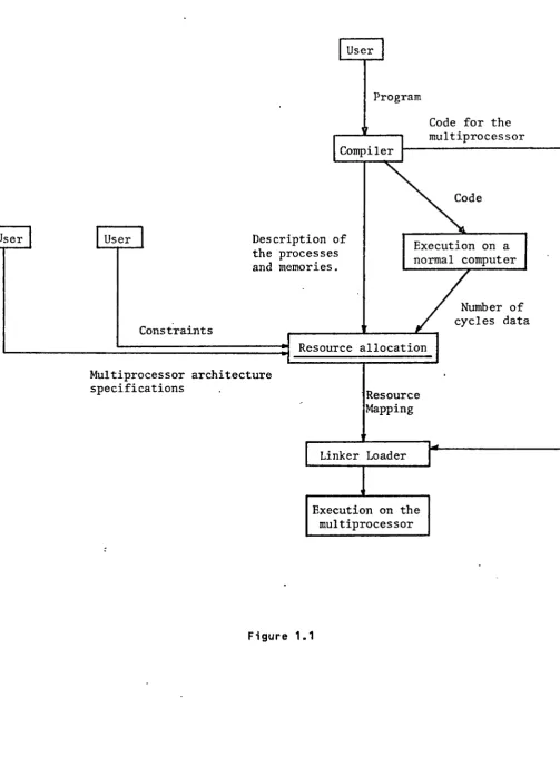
User
Program
Code for the multiprocessor Compiler
User Description of
the processes and memories.
Execution on a normal computer
Constraints
Multiprocessor architecture specifications
Resource allocation
Resource Mapping
Linker Loader
Execution on the multiprocessor
Figure 1.1
[image:12.564.30.534.83.772.2]Each address space must be assigned to some single physical memory space. There can be no overlap with any other simultaneously present address space.
Each process must execute from a processor which can access ell of the stores to which the address spaces accessed by the process have been allocated.
This concludes the definition of the basic terminology. The concept of resource allocation and is application areas have been introduced. Given such a utility and starting with a suitable application there are a number of stages involved in using it in order to implement a problem onto a multiple microprocessor. Figure(1.1) represents this information flow digrammatically.
(1.6) HIGH LEVEL LANGUAGES
---Firstly the problem needs to be implemented as a concurrent program. The advantages of using a high level Language for any programming is well documented [ 15,18,35,93,94). In view of this, and the fact that the resource allocator would itself be a complex program utility designed to aid program production, it is reasonable to
developm~nt of the user program will always utilize Language. Thus the resource allocator will always be compiler.
assume that the a high Level preceded by a
concurrent processes. The languages also provide some mechanism for communicating between two processes and for the sharing of data. Most of these languages that include processes will also have modules. The definition of a module is different for each author and language~ with some examples being presented in [ 16,41,49,64,67,68,69]. However in most cases the compiler can implement the module as a collection of procedures and variable spaces. So generally the use of modules has no effect upon the application of a resource allocator, which deals with variables and procedures and the access paths between these. However if the computer architecture supports modules directly, as in the Monads architecture [ 50,51] or the StarOS system [ 25,26], this poses no essential problems. In this case the resource allocator would deal with modules that have access paths between modules, as well as variables and processes. Nevertheless, to simplify the research, modules are not considered further.
(1.7) ARCHITECTURE SPECIFICATION
---When used the allocator requires the specification of the structure of both the program and the architecture. The program structure is best described by the compiler in terms of its process and address space elements and the access paths between these. The num~er of cycles information for the throughput calculations will be obtained by running the program on a normal uniprocessor computer. The code would be argumented with statements to gather statistics about the number of accesses made. This step is important as without the number of cycles information there is no feasible method for the resource allocator to obtain relative efficiencies of differing resource allocations.
The user is required to give a description of the computer
architectu~e to the allocator. The information that needs to be conveyed concerns such things
as-The kinds of processors, including their cycle speeds and microprocessor type.
The locatfons of memory mapped I/O, end the port addresses of nonmemory mapped I/O, as well as the processors which have access to these.
The addresses of interrupts, end the processors to which these interrupts occur.
The interconnection pattern between the processors and their stores. This will cover hardware buses and also the locations in the addressing range of a processor of its attached memories.
Only this level of information is required. Greater detail
about the hardware, as is given in many computer hardware design languages (a survey of these is given in [ 59,87J) is not required by the allocator end so is not supplied in this specification.
(1.8) PROGRAM SPECIFICATION
===========================
The specifications of the computer architecture need only be produced once per architecture, and used for the allocation of all programs to this architecture. Extra information is however required for each program. The user can interact with the resource allocator to guide it in its allocation strategy. The initial starting point for this is the description in [ 26, section 11J of the SterOS resource directives. These constraints may be to ensure that some conditions external to the allocator ere achieved, or to guide the allocator in its global strategy to achieve the most efficient mapping. The interaction takes place by the means of constraints placed upon the allocation. These constraints may be to
Ensure that processes execute upon processors that have hardware access to the appropriate I/O ports,
processor or store, or upon separate processors or stores. This ability is useful when using a multiprocessor to provide greater degree of computing reliability, one example of such a multiprocessor design being described in [ 6J. If different parts of a program are allocated upon separate physical resources, then a failure of one resource will only bring down one part of the program.
Allocate processes with special requirements to processors that possess special execution capabilities, such as a floating point accelerator.
Finally the resource allocator will operate upon this information and produce a resource mapping, or
possible. If the allocator succeeds
'
mapping. This would be used for1a load the program onto the machine.
(1.9) THE TOPICS RESEARCHED
---perhaps indicate that no mapping is then it will generate an allocation subsequent linker stage to actually
The research area and its application have been defined. The aim of this thesis is to investigate this problem, concentrating on the following topics
A) The computer specification language.
B) The throughput of the allocation mapping.
For its allocation activity the allocator will need to derive the throughput of an allocation, to decide if the allocation is efficient or not. Thus a general purpose throughput calculation algorithm is derived, which takes into account the effects of memory contention. Two different versions of this are implemented and examined. The original starting point for this work is from [ 44J which describes a general throughput calculation model that takes into account memory interference produced by a number of independent nonconcurrent programs executing on a multiprocessor. The thesis work extends this to include the effect of differing store cycle speeds, the effect of bus contention and bus cycle speeds, and to provide the throughput for a single concurrent program.
C) The allocation algorithms.
Finally the allocation algorithms themselves have been designed and an implementation produced to demonstrate them. This research borrowed ideas from search techniques developed in other areas, such as parallel searches in game trees [ 62J. It builds on the need for resource usage directives as described by [ 26J for the StarOS project.
A list of the original research performed follows •.
A) The design of the computer specification language is the authors own.
8) The original memory interference model is taken from [ 44J. The authors own original research is to modify this to suit the requirements of a resource allocator.
=====================
The remainder description of activity in more
of the thesis is concerned with an expanded this work. Chapter 2 introduces the resource allocation detail and describes some of the problems encountered in performing this.
Chapter 3 is concerned with the design of the specification language. This language is based upon a graph structure description of the computer architecture and allows the specification of the multiprocessor at the level of its processors, stores and bus interconnections. Chapter 4 discusses how this Language is used to describe to the allocator the various kinds of computer architectures that are Likely to be encountered.
Chapter 5 then describes how the computer program that is to be mapped onto the architecture is specified to the resource allocator. The extra information required of the user to guide the allocator is also introduced. No implementation of the specification language was attempted. While the ideas presented are important for the use of a resource allocator, ther·e are essentially no new difficulties in implementing such a Language once it has been designed.
given a particular resource allocation be calculated. Two alternative ways of one by a simulation model and one by a implementing both were developed to Chapter 6 describes how,
mapping, its throughput may computing this is presented, probabilistic model. Programs demonstrate their validity.
Chapter 7 is concerned solutions. This is basically search pattern designed to satisfactory solutions.
with the search method used to find a tree search with a heuristically ordered increase the probability of obtaining
CHAPTER (2)
===========
(2.1) AN OVERVIEW OF RESOURCE ALLOCATION
========================================
Simple applications of the resource allocation problem addressed by this thesis are described in the following.
The simplest example of resource allocation is the implementation of a program to execute on a uniprocessor system possessing a uniform memory structure. Even for concurrent programs this is readily achieved. The processes of the program execute on the same processor and can be managed by an appropriately written scheduler. Memory allocation schemes for a linear memory are well understood.
The addition of more processors, thus creating a multiprocessor computer architecture addressing a common memory, can also be handled relatively easily. One method is to construct a scheduler which allocates
of the
time slices on different hardware processors to the processes program as they become ready to execute. In this approach, the the computer programming system need not even be aware of the to a multiple processor architecture. Unfortunately, as the rest of
change
number of processors attach~d to a common physical memory increases, the amount of memory contention also increases. Eventually there comes a point of diminishing returns where the addition of an extra processor to the hardware will add only a marginal improvement to the throughput.
Many techniques may be used to alleviate this problem. Interleaved memories; separate memory modules, cache memories or memories that are faster than the processors are some possibilities. Hany of these memory designs are more applicable to large computers because of the cost of the associated hardware required to implement them. As well these solutions have the common characteristic of ignoring the specific structure of the programs being executed.
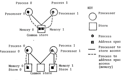
KEY
Processor 0 Processor 1
0
ProcessorD
StoreMemory 0 1
Common store G Process
fl
Address spaceProcess Process 1 Processor to
Processor 0 Processor 1 store access
Process to address space
Memory 1 access
Memory 0 (memory)
Store 0 Store 1
store
Figure 2.1
case there will be memory access conflicts when the two processors attempt to access the same store simultaneously in order to refer to their own memories. This situation is seen in the figure(2.1,top).
The memory interference may be reduced by the harcware techniques discussed above. Alternatively, if the structure of the program can be taken into account, on a suitable computer architecture the variable spaces could be placed into separate memory. blocks, as in figure<2.1,bottom). Now the interference due to accessing these memories will be nonexistent.
[image:20.565.135.546.75.346.2]patterns will be impractical. The research emphasis on medium sized statically allocated programs is a consequence of this.
(2.1.1) EXAMPLES OF RESOURCE ALLOCATION
As an example computer system
of resource allocation a simple instrument monitoring is used. This system i~ to monitor a number of instruments, and record their values in such a way that they can be retrieved upon command and displayed on a terminal. One way to structure a program to perform this action is to have an ind·ividual process obtain the results from each instrument and put these into a common table. Another process would be used to maintain the terminal display based upon the information in the table and according to user entered commands.
If it is assumed that the program work required to monitor a single instrument requires a significant part of the execution time of one individual processor, then a possible hardware implementation will have one processor for each of the instrument monitoring processes, and one more for the command process. This will give the best execution time performance for the complete program. Each processor can be supplied with its own private me~ory and also some global memory in common with all the other processors. For such an architecture as much as possible of the local address space of each process of the program would be assigned to the local physical memory of the processor. This will reduce the memory contention to the obligatory minimum, reducing it down to conflicting accesses by the processes to the address space that is shared with other processes. This hypothetical structure is depicted in the figure(2.2).
Private Stores
Global Store
Instrument Monitoring Multiprocessor
Figure 2.2
Processors Processors
Stores Stores
Figure 2.3
Both processors access STORE_3.
In figure(2.2) a homogeneous architecture has been proposed. It
could be possible to use different sized stores for each of the processors, and even to use different kinds of processors, thus creating a heterogeneous architecture. However it wil L generally be preferred to design and use homogeneous architectures, both because of an easier design stage, and also because such designs will more readily transfer to other projects.
To this structure the instrumentation input and output ports will be connected, with the ports for each individual instrument being connected to a separate processor.
Given nine instruments, a application is
PROGRAM MONITOR ;
COMMON DEFINITIONS ;
COMMON VARIABLES ;
PROCESS COMMAND ;
PROCESS INSTRUMENT_1
PROCESS INSTRUMENT __ 2
PROCESS INSTRUHENT_9
END ;
;
;
;
possible skeleton program for this
Each process will have a number of private variables and procedures, and the instrument processes communicate to the command process via a common table and common table access procedures.
Stores
Shared Stores
Global Store
Figure 2.4
appropriate to use a general purpose scheduler which allocates a ready process to a free processor as one becomes available.
If all of the I/O ports are not available from every processor then the user will be required to indicate to which processors the instrument monitoring processes are to be assigned. This is to ensure that each process is capable of accessing its correct instrument I/O ports. If this specification is imposed, then the resource allocator would then allocate the remaining control process to the best processor for it, which in this case will be the only unused processor available. Otherwise, if there are no such specifications, the allocation program allocate the program so as to obtain the best throughput, which in this computer architecture will imply one process per processor. At the conclusion of this activity the resource allocator will insert linking information into the compiler generated code to allow the code of the processes to access correctly their memory address spaces.
[image:24.567.88.461.75.289.2]process to a accessing this
physical memory and the number memory, can be reduced to
of different processes an unavoidable minimum.
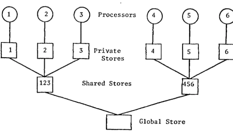
The resource allocator problem may easily become more complicated with only a few changes to the target architecture. For example a computer system with only six processors, each of which has access to all the required input ports, may be available to implement this program. Furthermore the memory may be arranged with a equal sized private memory attached to. each processor. Then each group of three processors would share a common memory block, and all processors would share a common global memory block. Such a design is given in figure(2.4).
The intent of constructing a computer system with these different levels of shared memory is twofold.
1. To increase the total amount of physical memory without exceeding the memory addressing range of any individual processor.
2. To allow the possibility of greater memory sharing between processors and yet still reduce memory contention.
In demonstration of this last point, processors 1, 2 and 3 can communicate between each other via the shared store 123 without interfering with processors 4, 5 and 6 in their accessing of their own shared store 456.
=================================
Now some of the factors that may affect the resource allocation placements will be considered.
(2.2.1) LOW LEVEL DETAILS
Firstly the resource allocation may be influenced by some machine Level details, such as the programmer inserting simple assembler Language routines to control input/output ports. Such information is not directly accessible to the resource allocator, but instead the user programmer will need to impose constraints upon the permissible mappings to guide the allocation activity in this area.
(2.2.2) PROCESS TO PROCESSOR ALLOCATION
In the instrument monitoring example, where the architecture of figure(2.4) is used, there are ten processors to be static~Lly assigned to the six processors. The allocator will tend to allocate the Longest running processes to separate processors, with the other Less time consuming processes placed where ever they fit. The Length of the run time of the processes is obtained by the execution of the program upon a normal computer and gathering statistics. However an allocation made in this way may not be optimal, depending on the combination of the particular program and computer architecture being used. So it will not always be the arrangement selected. This will be influenced by the effects of memory interference, different memory cycle times. of each physical memory block and of each shared memory bus, the size of the logical address space accessed by each process and the size of the physical memory shared by each processor.
(2.2.3) DEGRADATION DUE TO MEMORY INTERFERENCE
process A process B
process
c
,,.
I
I
'
\
-\
\
\
"
' '
'
'
...'
process C process V
Global Store
Figure 2.5
process A process B
3
\.
I
\
I
\
I
'
I
\ I
\
I
\ I
\ I
.
_...-
---...
-..
__
/Figure 2.6
...,.-/
6 Processors
Private Stores
Stores
KEY
rl
memory0
processproc~ss D
6 Processors
\
\
\
PrivateI
StoresI
I
/
/
Stores/
/
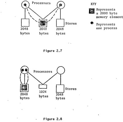
201\8
bytes
2048
bytes
bytes
2048 bytes
Figure 2.7
bytes 2048 bytes
Figure 2.8
Stores
Stores
m
HcprcsentsllR a 2000 byte memory clement 0 Represents
one process
pairs of .processes, each pair their own heavily used1
data ·section. The pair A and B could be assigned to any of the processors 1, 2 or 3, and their shared data\ space A placed upon the shared store of these processors. The other pair can be similarly assigned to the processors
4,
5 or 6. With such an allocation the pairs of processes can access their own shared address spaces without interference. This situation is represented in figure(2.5).However, if each process had been assigned so that the first process of the pair is in the processor group 1 to 3, and the second process of the pair is in the other processor group, as 1n figure(2.6), then the common shared data\ will have to be assigned to the global memory store. This assig~ment will inevitably result in greater memory conflict.
[image:28.564.109.510.51.450.2]<2.2.4) ALLOCATION INTERACTIONS
A final difficulty in the allocation process is the interactions that occur between individual allocations of program elements to resources. These interactions frequently prevent any straight forward allocation strategy, and will often prevent the most efficient usage of the computer architecture. As an example, for a two process program the best allocation onto a two processor architecture is to have a process assigned to each processor, shown in figure(2.7).
However the common address space element may not be allowed onto the common store. This will happen if the size of the common address space is larger than the size of the common store. Therefore the common address space now has to go into one of the private physical memories. In order to access this, both processes will then end up on the same processor, with the othe~~processor idling. This is depicted in figure<2.8), where the common store has a reduced size of 1024 bytes.
A similar situation can occur easily with the allocation of address spaces to stores. The difficulties also increase when memory and bus contention is to be taken into account. These interactions may be caused by other factors, and can affect the allocation strategy of the whole program.
Because of these interactions the allocation problem is nonlinear, it is not possible to work out the allocation for individual parts of the given problem and then to combine these to give a complete allocation. In most cases it will unfortunately turn out that the allocations for one part will inter.act with the allocations in all of the other parts, so completely invalidating any such divide and conquer solution.
(2.2.5) RESOURCE ALLOCATION FAILURE
size of the program.
The physical memory addressing range of a processor exceeds the address space sizes of all the processes that are required to execute upon it.
A process is assigned to a processor so that it cannot access the stores to which its address spaces have been assigned.
A process or address space element is where it cannot access its I/O ports ports).
(2.3) SOME RESOURCE ALLOCATION APPLICATIONS
===========================================
assigned to a resource (or memory mapped I/O
The introductory examples given so far have given some of the basic requirements, and some of the problems confronting a resource allocator have been demonstrated. In the following more example applications are introduced.
(2.3.1) PICTURE PROCESSING
Main Processors .
Local Memory
Local Memory
given in figure(2.9).
Global Memory
Figure 2.9
The user will need to provide constraints which will place the picture processes onto the picture processors, and supply the additional information that the code for the picture processors has to be compiled into a different instruction set from the code for the main processors. The user is also required to supply specifications of the computer architecture. Then using these user directives and the specifications, the resource allocator will be able to perform the rest of the· allocation for a suitably constructed program automatically.
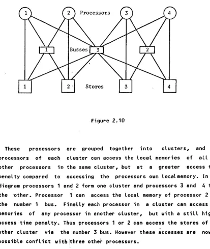
(2.3.2) CH* TYPE COMPUTER ARCHITECTURE
Stores
Figure 2.10
These processors are grouped together into clusters, and the processors of each cluster can access the local memories of all the other processors in the same cluster, but at a greater access time penalty compared to accessing the processors own localmemory. In the diagram processors 1 and 2 form one cluster and processors 3 and 4 form the 'other. Processor 1 can access the local memory of processor 2 via the number 1 bus. Finally each processor in a cluster can access the memories of any processor in another cluster, but with a still higher access time penalty. Thus processors 1 or 2 can access the stores of the other cluster via the number 3 bus. However these accesses are now in possible conflict with ~hree other processors.
I
[image:32.560.68.482.86.576.2]Processor
store
Processor
store Common store
Common store
Processor
Processor
store
Processor
Private store
Figure 2.11
Processor Processor
store
Common
store store
Common store
Figure 2.12
Processor
Private store
Processor
Common store
Processor
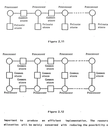
important_ allocation
to produce an efficient will be mainly concerned
implementation. The resource with reducing the possibility of memory conflicts.
(2.3.3) SYSTOLIC ARCHITECTURE
[image:33.565.48.507.62.605.2]neighbours via the common physical memory elements. Such architectures are useful when the applications problem can be split into a number of stages of roughly equal computing load, and each stage can follow on from the one before it. One such application is in three dimensional computer graphics, where a program may be divided into processes to
Perform object ordering in depth first order. Elimination of objects entirely out of view. Removal of polygon faces facing the wrong way.
Three dimension to two dimensional coordination transformation. Hidden line elimination.
Final drawing of the lines onto the screen.
CHAPTER (3)
===========
(3.1) INFORMATION SPECIFICATION LANGUAGE
========================================
The information specification language (ISL) allows a machine understandable definition of a computer architecture to be constructed. It also provides the user with the facilities to guide the resource allocation activity.
This chapter will describe the basic underlying graph structure of this language, and introduce the parts of the Language concerned with
~
the definition of a computer architecture. The reference text used for the basic graph theory is [ 48J.
(3.1.1) UNDERLYING INFORMATION STRUCTURE
Starting with a denumerable set X=<X1,X2, ••• Xn} and a mapping H of X into X, a graph is the pair G=<X,H).
The ISL associates two functions with the set of elements of such a graph. One function is a mapping Fv from the set
V=<null,V1,V2, ••• }. This is called the value
X to the set V, where function. The other function is a mapping Fn from the set X to the set N, where N=<null,N1,N2, ••• }. This is called the name function.
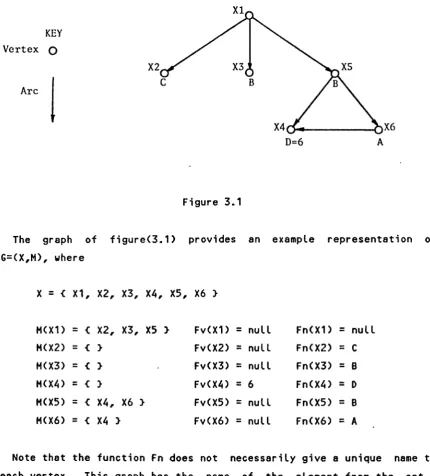
A graph can be represented on paper by drawing vertices and arcs. A vertex is drawn as a point and corresponds to an element in X. A directed arc is drawn as an arrow from one vertex to another vertex. A directed arc exists from vertex Xi towards Xj if Xj is in the set M(Xi).
The value and name of each vertex may be represented also. If the name function fn(Xi) of vertex Xi is nonnull, it is written alongside the vertex. If the value function Fv(Xi> of vertex Xi is nonnull, it is also written alongside the vertex. If both the name and value functions are nonnull, then the
followed by an = and
representation of the name is then the written representation
Vertex 0
Arc
!
X6D=6 A
Figure 3.1
The graph of figure(3.1) provides an example representation of G=<X,H), where
X =
<
X1, X2, X3, X4, XS, X6 }H(X1) = { X2, X3, X5 } Fv(X1) = null FnCX1) = null
H<X2) = { } FvCX2) = null FnCX2) =
c
HCX3) = { } Fv(X3) = null Fn(X3) = B
HCX4) = { } FvCX4) = 6 FnCX4) = D
HCX5) = { X4, X6 } FvCX5) = null FnCX5) = B
HCX6) = { X4 } FvCX6) = null Fn(X6) = A
Note that the function Fn does not necessarily give a unique name to each vertex. This graph has the name of the element from the set X written next to each vertex. In general this set identification is not needed in subsequent discussions about the ISL and so will rarely be mentioned after this section.
A directed arc U is represented by the pair CXi,Xj). Xi is called the initial extremity of the arc and Xj is called the terminal extremity. An arc U is connected to e yertex Xi if U=<X,,Xn) or if U=(Xn,Xi), Xi<>Xn. A directed path is a finite sequence of arcs
[image:36.558.63.494.76.553.2]A vertex Xj is attached to vertex Xi if Xj is a member of H(Xi). The attached vertices of Xi are ell Xj such that this condition holds.
Given a vertex Xi, the connection set C of Xi is the set of all the vertices Xj, Xj<>Xi, such that there exists a directed path from Xi to Xj. In the figure some connection sets are
C(X1)
=
<
X2, X3, X4, X5, X6 } C(X2)= { }
C(X5)
= {
X4, X6 } C(X6)= {
X4 }Any vertex Xi in the graph G, which is not in any set H(Xj), is called a root of the graph. That is there are no arcs whose terminal extremity coincide with a root vertex. In the example graph of figure(3.1), the vertex X1 is the root.
The graphs used by the ISL have some common properties. There is always one and only one root. If Xi is a vertex in the graph G, then there will always exist a directed path from the root vertex to Xi. Thus the connection set C(Xr)=X, where Xr is the root vertex. For the root vertex Xr, Fn(Xr)=null and Fv(Xr)=null. For all Xi where Xi<>Xr, Fn(Xi)<>null and Fv(Xr) can be null or nonnull •
. In the following there ls a brief overview of how the ISL may be used to construct a graph structure, and how to access such a graph once it exists.
===========================================
In the ISL there are operations that allow a graph to be constructed, and sets of vertices from this graph to be specified. There are also the more conventional high level language features which provide for arithmentical expressions, program flow control and the like.
A graph defined by the ISL always starts from a root vertex, which Is denoted by a @character. Other vertices, which may be directly or
indirect-ly attached, can onindirect-ly be accessed via this root vertex. The simplest selection reference is
@
which will produce a reference set containing only the root vertex. The reference
@.N
will select all those vertices of name N that is attached to the root vertex.
Reference set variables may also be used, thus
V := @.N
will assign to the reference set Vall the vertices named N that are attached to the root vertex. Now the reference expression
V.M
will generate the set of all the vertices of name M that are attached to any of the vertices in the reference set V. This is equivalent to the reference set expression
@.N.M
@.A.<NOT_EMPTY (@.B)>
will select only those vertices of name A Which are attached to the root vertex, which themselves have one or more vertices of name B attached. Another example Is
@.A.<NUMBER (@.B) = 2>
which will select only those A vertices which have exactly two B vertices attached.
Having selected a set of vertices, they may be used to create new edges in the graph, as in
@.A.B -> @.A.C
This will attach every C vertex defined in the second reference set expression to every B vertex defined in the first reference expression.
Figure E.8 shows a diagram of this.
As well, new vertices may be created by using the NEW operation, as in
@ -> NEW ( A=3 )
which will create a new A vertex, give it a value of 3, and attach it to the root vertex. Another example is
@ -> (NEW(A), NEW(A), NEW(B))
which will create two new A vertices and one new B vertex, and attach them to the root vertex.
Program flow control constructs are provided to Implement FOR loops and IF conditionals. As an example, the creation of three new D vertices might be achieved by
An example of a conditional statement Is
IF 1 > 2 THEN
@ -> NEW(A} END ;
CHAPTER (4)
---(4.1) USING THE INFORMATION SPECIFICATION LANGUAGE GRAPHS
=========================================================
Computer architecture specifications are used to specify the architecture of a (possibily multiprocessor) computer to the resource allocator. This information allows the allocator to deal with the allocation of code and data parts of a program onto the hardware processors and memory elements of the computer system.
For this purpose the of the computer
resource allocation algorithms required a model system which contains information about the
Address ranges and sized of the physical memory elements, The names of the processors,
The cycle speeds of the memories and processors, The interconnections between processors and memories, Information about the I/O system and interrupt addresses,
However there is no need for further knowledge of the system architecture in terms of registers, data and address buses or detailed knowledge of the input and output logic.
===============================================
(4.2.1) A SIMPLE SYSTEM
The simplest computer system is one processor connected to a single memory unit. This can be described by
GRAPH BEGIN
S -> NEW ( PROCESSOR ) -> NEW ( ADDRESS ) ; END ;
This specifies to the resource allocator that a computer architecture has a processor and a memory module. The address range which the processor refers to the memory unit will be given by extra vertices attached to the address vertex. In subsequent specifications, to refer to the processor the reference used is
~.PROCESSOR
and to refer to the address range the reference used is
&.PROCESSOR.ADDRESS
The resource allocator will recognize the PROCESSOR identifier to be one of the standard identifiers which in
hardware processor. Such processors directly understood by the allocator.
this case refers to an actual can have properties that are This information includes the processors name and its cycle speed and this is represented by vertices attached to the PROCESSOR vertex. These have the standard names NAME and CYCLE. They may be defined for the example system as
GRAPH BEGIN
i -> NEW ( PROCESSOR ) ->
( NEW ( ADDRESS ) ,
NEW ( CYCLE
=
2.5 ) ) ; END ;The PROCESSOR -definition is as before. This vertex now has attached to it two new vertices, one called NAME and the other called CYCLE. They convey information about the name of this processor, BRANDX, and its cycle time, 2.5 microseconds. These values can be referenced by
VALUE ( @.PROCESSOR.NAME ) VALUE ( i.PROCESSOR.CYCLE )
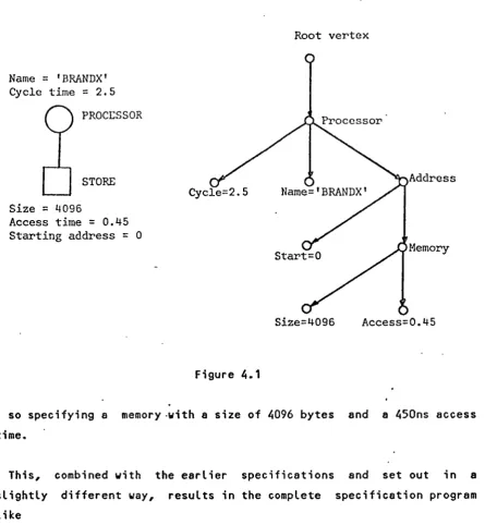
(4.2.2) SPECIFYING MEMORY
Vertices named ADDRESS and PROCESSOR are directly understood by the allocator. It expects the ADDRESS vertex to have two further standard vertices attached. One vertex is called START and this has an integer value giving the start address at which the processor accesses the first memory byte of the memory module. The other vertex is called MEMORY and this vertex represents information about the physical memory module. This vertex has attached to it two further vertices, calle~ ACCESS and SIZE. The ACCESS value gives the access time of the memory in microseconds, while the SIZE value gives the size of the memory in bytes. The ACCESS and SIZE vertices are not attached directly to the ADDRESS vertex, since different processors may have different address ranges in which they access this same memory.
As an example already defined
a memory unit of 4096 bytes for the computer system can be specified by the addition of the statements
i.PROCESSOR.ADDRESS ->
( NEW ( START
=
0 ) , NEW ( MEMORY ) ) ;This attachs two new vertices to the ADDRESS vertex. They are START and MEMORY, the START vertex has the value of O. Information for the MEMORY vertex is further specified by
i.PROCESSOR.ADDRESS.MEHORY ->
Name
=
'BRANDX' Cycle time=
2.5PROCI:SSOR
STORE
Size
=
4096Access time
=
0.45 Starting address=
0Address
Memory
Size=4096 Access=0.45
Figure 4.1
so specifying a memory -with a size of 4096 bytes and a 450ns access
time.
This, combined with the earlier specifications and set out in a
slightly different way, results in the complete specification program
like
GRAPH
CONST NAME_VALUE
=
'BRANDX' ,CYCLE_VALUE
=
2.5 ; · BEGIN6l -> NEW ( PROCESSOR ) ->
( NEW ( CYCLE
=
CYCLE_VALUENEW ( NAME
=
NAME_VALUE )NEW ( ADDRESS ) -> ( NEW ( START
=
0 ),
NEW ( HEMORY ) ->
)
,
,
( NEW ( SIZE
=
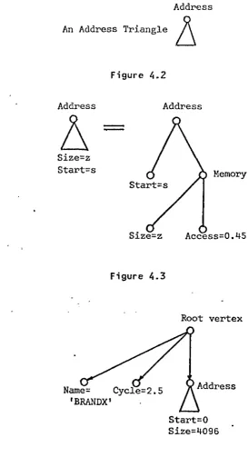
4096 ) , [image:44.557.68.514.59.542.2]Address
An Address Triangle
~
Figure -4.2
Address Address
Size=z Start=s
-
[image:45.558.123.397.72.587.2]
-Size=z
Figure 4.3
Name= Cycle=2.5
'BRANDX'
Figure 4.4
Memory
Access=0.45
Root vertex
•·
) )
END ;
)
Start=s Size=z
.·
Address
Memory
Size=z Access=0.45
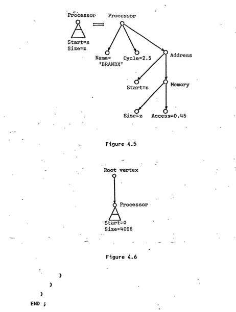
Figure 4.5
Root vertex
Start=O Size=4096
Figure 4.6
Thus this represents a computer architecture with a processor called
BRANDX having a processor cycle time of 2.5 microseconds. This processor has access to 4096 bytes of 0.45 microsecond store attached, with the
store occupying the first 4096 bytes of the processors addressing range.
[image:46.557.37.500.61.674.2]To reduce the size of the graph diagrams in the following text, a visual shorthand representation is used. A triangle like that of figure(4.2) is called an address triangle. It is taken to represent an ADDRESS vertex and all of the vertices that are shown in figure(4.1) to be attached to this ADDRESS vertex. Its equivalent graph is given in figure(4.3), using this the graph of figure(4.1> can be redrawn as shown in figure(4.4). The SIZE and ADDRESS vertex values are given under the triangle. These are only specified in the following graphs if their values are important for the ISL example being demonstrated. Otherwise they are not explicitly mentioned.
An even more compact representation of the graph of figureC4.1> is provided by using a processor triangle defined as in figureC4.5). In
figureC4~'6) the graph of figure(4.1> has been redrawn this way. As with the memory triangle, the values of the vertices that have values
,
attached are only explicitly provided if it is required for the example demonstration.
C4.2.3) MULTIPLE MEMORIES
In more complex computer systems a processor may access mor.e than one memory module. This is represented in the specifications by attaching more than one ADDRESS vertex to the same PROCESSOR vertex. The address vertices
address ranges modules.
of a particular processor must and will generally have access
have nonoverlapping to different memory
An extra memory may be added to the computer system defined above by adding the specificat~on
&.PROCESSOR ->
( NEW ( ADDRESS ) ->
) ;
( NEW ( START
=
4096 ) , NEW ( HEHORY ) ->( NEW ( SIZE
=
4096 ) , NEW ( ACCESS=
0.45 ) ))
Processors
Processor Stores
Figure 4.7
with name ADDRESS. This is depicted in figure(4.7>.
Note that here the extra memory is represented by attaching the address triangle to the PROCESSOR vertex to which the processor Triangle is attached Address vertices are always attached to the processor vertex if that processor accesses the memory, so this is possible.
The reference
S.PROCESSOR.ADDRESS
will refer to both address vertices, and the reference
S.PROCESSOR.ADDRESS.HEHORY
will refer to both of the memory modules.
To refer to only one of the address vertices indexing may be used. Thus to refer to the second memory module requires the reference