Effects of Stratification and Flows on P-1/P-2 Ratios and Anti-node Shifts Within Closed Loop Structures

Anti-node Shifts Within Closed Loop Structures

.

White Rose Research Online URL for this paper:

http://eprints.whiterose.ac.uk/106794/

Version: Accepted Version

Article:

Erdelyi, R., Hague, A. and Nelson, C.J. (2014) Effects of Stratification and Flows on

P-1/P-2 Ratios and Anti-node Shifts Within Closed Loop Structures. Solar Physics, 289 (1).

pp. 167-182. ISSN 0038-0938

https://doi.org/10.1007/s11207-013-0344-2

Reuse

Unless indicated otherwise, fulltext items are protected by copyright with all rights reserved. The copyright exception in section 29 of the Copyright, Designs and Patents Act 1988 allows the making of a single copy solely for the purpose of non-commercial research or private study within the limits of fair dealing. The publisher or other rights-holder may allow further reproduction and re-use of this version - refer to the White Rose Research Online record for this item. Where records identify the publisher as the copyright holder, users can verify any specific terms of use on the publisher’s website.

DOI: 10.1007/•••••-•••-•••-••••-•

Effects of Stratification and Flows on P1/P2 Ratios

and Anti-Node Shifts within Closed Loop Structures

R. Erd´elyi1 · A. Hague1 ·C. J. Nelson1,2

c

Springer••••

Abstract The solar atmosphere is a dynamic environment, constantly evolv-ing to form a wide range of magnetically dominated structures (coronal loops, spicules, prominences, etc.) which cover a significant percentage of the surface at any one time. Oscillations and waves in many of these structures are now widely observed and have led to the new analytic technique of solar magneto-seismology, where inferences of the background conditions of the plasma can be deduced by studying magneto-hydrodynamic (MHD) waves. Here, we generalise a novel magneto-seismological method designed to infer the density distribution of a bounded plasma structure from the relationship of its fundamental and subsequent harmonics. Observations of the solar atmosphere have emphatically shown that stratification, leading to complex density profiles within plasma structures, is common thereby rendering this work instantly accessible to solar physics. We show, in a dynamic waveguide, how the period ratio differs from the idealised harmonic ratios prevalent in homogeneous structures. These ratios show strong agreement with recent observational work. Next, anti-node shifts are also analysed. Using typical scaling parameters for bulk flows within atmospheric waveguides,e.g., coronal loops, it is found that significant anti-node shifts can be predicted, even to the order of 10 Mm. It would be highly encouraged to design specific observations to confirm the predicted anti-node shifts and apply the developed theory of solar magneto-seismology to gain more accurate waveguide diagnostics of the solar atmosphere.

Keywords: Oscillations, Solar; Waves, Magnetohydrodynamic; Waves, Propa-gation.

1. Introduction

The ubiquitous magnetic fields within the solar atmosphere create a vast array of, often dynamic, plasma structures, such as coronal loops and spicules, which are

1

Solar Physics and Space Plasma Research Center, University of Sheffield, Hicks Building, Hounsfield Road, Sheffield, S3 7RH;

Email: (robertus; sma08abh; c.j.nelson)@shef.ac.uk

2

known as ‘waveguides’ for magneto-hydrodynamic (MHD) waves. Such waves have been widely studied in recent years due to the potential that they may contribute non-thermal energy to heating the corona (for a review of MHD waves, see: Roberts, 2000; Ruderman and Erd´elyi, 2009; Taroyan and Erd´elyi, 2009; Mathioudakis, Jess, and Erd´elyi, 2012). In this article we focus our attention on a thin, finite-length, magnetic string, analogous to a coronal loop, to study how density stratification effects the relationship between the fundamental (first) and subsequent harmonics in a dynamic waveguide.

Oscillations in magnetic, cylindrical structures were extensively studied, and summarised in a recently popular form, in a theoretical capacity, by Edwin and Roberts (1983) and Roberts, Edwin, and Benz (1984). However, it was not until Aschwandenet al.(1999) interpreted coronal loop oscillations, viewed using the

Transition Region and Coronal Explorer (TRACE) satellite, as manifestations of the fast kink-mode that they were first observed. Recent improvements in spatial and temporal resolutions have allowed a large number of oscillations to be observed, e.g., Alfv´en waves first observed by Jesset al. (2009) in the lower solar atmosphere (for a review see Mathioudakis, Jess, and Erd´elyi, 2012); kink waves (Aschwandenet al., 1999; Verwichteet al., 2004; see Andrieset al.(2009) for a review); longitudinal waves (Deforest and Gurman, 1998; Berghmans and Clette, 1999; reviews of sausage modes include De Moortel (2009) and Wang (2011)). In particular, Verwichteet al.(2004) claimed to have observed evidence of the first harmonic of an oscillating coronal loop; a potentially important tool for solar magneto-seismology.

A plethora of examples of the fundamental and first harmonic within an active region have been reported in recent years (e.g., De Moortel and Brady, 2007; O’Shea et al., 2007). Analysing a variety of TRACE observations, Van Doorsselaere, Nakariakov, and Verwichte (2007) reported P1/P2 ratios of 1.81, 1.58 and 1.795 for fast kink-mode oscillations within coronal loops. Srivastava

et al. (2008) used Hinode data to calculate a P1/P2 ratio of 1.68 for sausage modes in cool post-flare chromospheric loops. One suggested reason for the de-viation of these values from two (the P1/P2 ratio for a homogeneous flux tube) is density stratification, where complex interactions of gravity and magnetism lead to inhomogeneity within the tube. Inhomogeneity within tubes may also lead to

spatial periodicities. Jess et al. (2008) analysed the same data as Aschwanden

et al. (1999), finding spatial periodicities over length scales of, approximately, 3.5 Mm. Observed period ratios within sunspot umbrae have been studied by Campos (1986) (including the P1/P2 and P1/P3 ratios) finding deviations from homogeneous values, implying that analytical approximations for thin-tubes should be extended to thick-tubes. The P1/P2 ratio has been widely applied in recent years, for example, Andries, Arregui, and Goossens (2005) and Verth, Erd´elyi, and Jess (2008) were able to estimate the scale height of a coronal loop; the latter even considering the significance of magnetic stratification.

the context of solar interior-atmospheric magnetic coupling, by Erd´elyi (2006), to any magnetised solar plasma structure. There are several examples of this method being exploited including Nakariakov and Ofman (2001) and Erd´elyi and Taroyan (2008). Verth et al. (2007) used spatial magneto-seismology to calculate the anti-node shift of a magnetic flux tube with a non-homogeneous density stratification. Further examples of magneto-seismology can be found in, for example, Soler and Goossens (2011) and Soler, Ruderman, and Goossens (2012). However, we expand upon these works by finding analytical approxi-mations for specific density profiles that may model, and give insight, to the complex stratification of atmospheric waveguides.

D´ıaz, Oliver, and Ballester (2010) discussed a step-function density within a loop structure, modelling the large density gradient between its footpoint and apex, finding that for large density jumps a bead which is close to the centre of a magnetic structure, representing dense prominence threads, will be observed to haveP1/P2<2. Soler and Goossens (2011) expanded this work to a flowing heavy thread, where the period ratio was calculated numerically, also finding a fall from the canonical value of two. In this work, we discuss a bead, analogous to a ‘blob’ of plasma propagating slowly along a coronal loop such that ρthread ≈ ρbead (observed by, for example, Ofman and Wang, 2008). We assume that the bead is close to the end of the tube (rather than in the centre as studied in, e.g., D´ıaz, Oliver, and Ballester, 2010), as the largest divergence from the homogeneous harmonic ratio should occur in spatial positions close to the end of the loop. We begin by formulating an analytical solution for a light bead which is stationary and situated close to the end of the loop. This is then expanded so that the bead may move slowly away from the end of the loop, simulating flows observed within coronal loop structures. A comparison between these results and numerical results is also made.

Recent high-cadence, high-resolution observations have led to discussions re-lating to the idea of flows within coronal loops (see, Kopp et al., 1985; Ofman and Wang, 2008). Often, localised brightenings can be observed progressing along loop structures from the footpoints in the photosphere and chromosphere into the corona (see,e.g., Ofman and Wang, 2008). How these localised flows influence MHD modes within loop structures has initially been studied in,e.g., Soler and Goossens (2011) and Soler, Ruderman, and Goossens (2012) in ideal MHD and by Morton and Erd´elyi (2009) for cooling coronal loops. It has been found that small, propagating density structures within loops can cause a deviation from the expected canonicalP1/P2 ratio. We study such a system. Further, the topic of anti-node shifts is also discussed, finding that non-homogeneous density profiles lead to large divergence from expected anti-node positions. The underpinning idea here is that eigenfunctions may be more sensitive to small (i.e., linear) perturbations when compared to variations in eigenvalues (i.e., frequencies) of MHD waveguides.

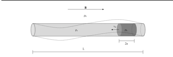
Figure 1. A schematic diagram of the model presented. For Section 4,v0 = 0. The dashed

line represents the first harmonic standing oscillation of a homogeneous loop.

Section 5. In Section 6, the anti-node shift of the harmonics is discussed in the context of spatio magneto-seismology. Section 7 draws together our conclusions and suggests further research.

2. Model Setup

The model which is studied can be summarised as the oscillations of a straight-ened, thin flux tube of length L and radius R. We use a cylindrical coordinate system (r, ϕ, z) where thez-axis corresponds to the axis of the tube. The mag-netic field both inside and outside the tube has the form B=Bez where B is

homogeneous with respect toz. As in many coronal models, theβ = 0 (i.e., cold plasma) condition is applied, thereby removing any dependency on temperature. The loop has footpoints fixed in the photosphere,i.e., its ends are immovable at

z= 0 andz=L.

We state that ρe is the background density of the tube and ρb(= ρe +δρ

where |δρ| ≪ |ρe|) is the density within the bead. The tube sits within a quiet coronal plasma with density,ρo, much less than the tube densityi.e.ρo/ρe≪1. The bead moves with a constant speed,v0. The setup of the problem is shown in Figure 1. This model represents an oscillating coronal loop in which plasma, of a higher density than that of the loop, moves along the magnetic field lines, modelling observations by, e.g., Ofman and Wang (2008).

these are thought to be more realistic of solar structures. However, a combination of flows and continuous density profiles present numerous difficulties which are not studied in the present article. The expansion of the methods presented in this research to more complex geometries could form the basis of an interesting future study.

It is assumed that the tube exists such that it can be modelled by the thin-tube approximation (TT) outlined by Dymova and Ruderman (2005)i.e.R/L≪1. Assuming a typical coronal loop structure, we estimate thatL≈50−150 Mm andR≈1−2 Mm givingR/L≈0.007−0.04 and, hence, that this approximation holds for our model. From this approximation, Dymova and Ruderman (2005) found that the governing equation (which has later been used by, e.g., Erd´elyi and Verth, 2007; Verth and Erd´elyi, 2008) of transversal perturbations can be written as

∂2_{v(z, t)} ∂t2 −v

2 k(z, t)

∂2_{v(z, t)}

∂z2 = 0, (1)

wherev(z, t) is the transverse velocity at the tube boundary, andvk(z, t) is the kink-speed defined as

vk,e(z, t) =

s

2B2

µ(ρe+ρo) and vk,b(z, t) =

s

2B2

µ(ρb+ρo). (2)

Note, asδρ→0, it is simple to see thatvk,e(z, t)≈vk,b(z, t).

Equation (1) is only strictly applicable whenvk is independent oft,i.e.there are no bulk motions present. The correct equation, taking into account bulk flows, was derived by Ruderman (2010); however, in a suitable limit (v0≪vA, the Alfv´en speed), Equation (1) is applicable and has been widely used by,e.g., Soler and Goossens (2011).

3. Single Density Discontinuity

We begin our analysis by considering a single density jump; this can be mod-elled using a Heaviside function. Let us assume that the density,ρ, follows the distribution

ρ(z) =

ρe z∈[0, z0];

ρb z∈[z0, L], (3)

wherez=z0is the position of the density jump andρe< ρbimplies 0< δρ(or

ρb< ρe thatδρ <0).

To calculate the dispersion relationship for standing waves with these back-ground conditions, we will use the separation of variables technique on the governing equation [Equation (1)], assuming thatv(z, t) =Z(z)T(t).The spatial dependence,Z(z), is denoted by

Z(z) =

Ze(z) z∈[0, z0];

where

Ze(z) =Asin

_ωz

vk,e

(5)

and

Zb(z) =C

sin

ωz vk,b

−tan

ωL vk,b

cos

ωz vk,b

, (6)

are calculated using the boundary conditions. We shall define two further con-ditions on the oscillating loop

[Z(z)]z=z0+δz

z=z0₋δz= [Z

′_(z)]z=z0+δz

z=z0₋δz= 0, as δz→0, (7)

thereby forcing continuity of the waveguide at z0. Applying these conditions to Equations (5) and (6) gives us the dispersion relationship,

tan

_ωL

vk,b

tan

_ωz0

vk,e

tan

_ωz0

vk,b

+

_vk

,b vk,e

+

tan

_ωz0

vk,e

−

_vk

,b vk,e

tan

_ωz0

vk,b

= 0. (8)

In order to reduce the trigonometric equation [Equation (8)] to a simpler approximation of ω, dimensionless parameters, as in Verth et al. (2007), are introduced. This allows us to replace the characteristic speed, the eigenfrequency,

ω, andz0 with their scaled counterparts

κ=

_vk

,b vk,e

, γ= ωL

vk,e

, ǫ= L−z0

L . (9)

Using the dimensionless parameters [Equation (9)] and Equation (8), we are able to calculate

tanγ

κ

=

κtanωz0

vk,b

−tanωz0

vk,e

tanωz0

vk,e

tanωz0

vk,b

+κ, (10)

tan (γǫ) =

tan (γ)−tanωz0

vk,e

1 + tan (γ) tanωz0

vk,e

, (11)

and

tanγǫ

κ = tan γ κ

−tanωz0

vk

,b

1 + tan γ_κ

tanωz0

vk,b

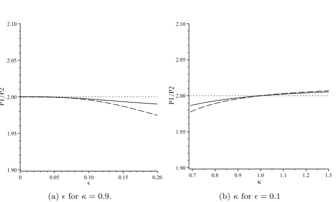
(a)ǫforκ= 0.9. (b)κforǫ= 0.1

Figure 2. Fits of the analytical solution derived in Equation (20) to numerical models.

After some further algebra, Equation (8) can be cast into the following, more compact, form,

[tan(γ)−tan(γǫ)] +κhtanγǫ

κ

+ tanγǫ

κ

tan(γ) tan(γǫ)i= 0. (13)

Assuming a weak stratification, such that ρe ≈ ρb, it is simple to see that

κ≈1. Equation (10) implies

tan(γ)≈0, (14)

and so

γ≈nπ, n= 1,2,3, ... (15)

Acknowledging the basic model setup of the geometry of the problem, we limit the spatial position of the discontinuity such that ǫ ≪ 1. Simple calculations then lead us to

tan(γ)≈γ−nπ, (16)

tan(γǫ)≈γǫ+1 3(γǫ)

3_{, (17)}

tanγǫ

κ

≈ γǫ κ +

1 3

γǫ

κ

3

, (18)

which allow us to rewrite Equation (13) as a cubic function in γ. Since ǫ is, by definition, small, O(ǫ4_{) or higher order terms have been neglected from}

relationship

ǫ2

1 3 ǫ−ǫκ

2

+κ2

γ3−(ǫκ)2nπγ2+κ2γ−nπκ2= 0. (19)

The dispersion relation is now in a convenient form, as a wide range of methods are available for solving cubic equations, allowing Equation (19) to be solved for

γ. Using the perturbationγn=nπ+ ˜γ, we are able to analytically determineγ,

i.e.

γn =nπ+

ǫ3_n3_π3_(κ2₋₁₎

3(n2_π2_ǫ3_(1−κ2_{) +ǫ}2_κ2_n2_π2_+κ2₎, (20)

hence, allowing the calculation of theP1/P2 ratios for this density profile (asγ

is related toωthrough Equation (9), it is easy to see thatPn∝1/γn). Note that we have added the subscript nto γto denote the (n−1)-th harmonic clearly.

We are easily able to note, that ˜γ causes the deviation of the ratios of the harmonics for κ 6= 1, from the counterparts in uniform plasma. Let us plot

P1/P2 by fixing κ at, e.g., 0.9 and varyingǫ (Figure 2a) and fixing ǫ at, say, 0.1 while varying κ (Figure 2b). These choices of κ and ǫ represent a coronal loop embedded in the solar atmosphere. The period ratio is now calculated using Equation (20) (solid line); also plotted is the period ratio computed using numer-ical methods with respect to Equation (13) (dashed line). A strong correlation between the numerical and analytical solutions is observed for ǫ <0.2 (Figure 2a). This agrees with the assumption that ǫ ≪ 1. For ǫ = 0.1, the fit of the analytical and numerical solutions around κ = 1 shows less than one percent error (Figure 2b). Note that Figure 2b shows that for κ > 1, a lower density after the jump,P1/P2 >2. Forκ <1, corresponding to a higher density after the jump, P1/P2 <2; as in many observed kink mode oscillations of coronal loops (e.g., Van Doorsselaere, Nakariakov, and Verwichte, 2007). This model is rather basic and is not an accurate representation of observed density profiles. However, in this work, it serves as a basis to expand the analysis in future sections.

4. Step Function Density

Step function densities are models which can be used to approximate a range of observed phenomena within coronal loops. For example, a small bead propagat-ing from the footpoints in the photosphere or chromosphere to the corona along a waveguide (see Ofman and Wang, 2008) or stratification, where a two-layer atmosphere is chosen (i.e. a heavy photosphere and light corona leading to a decrease in density in the centre of the tube). The first example is analysed in this article. The analysis presented, focuses on a density profile defined as

ρ(z) =

ρe z∈[0, z0−a]∪[z0+a, L];

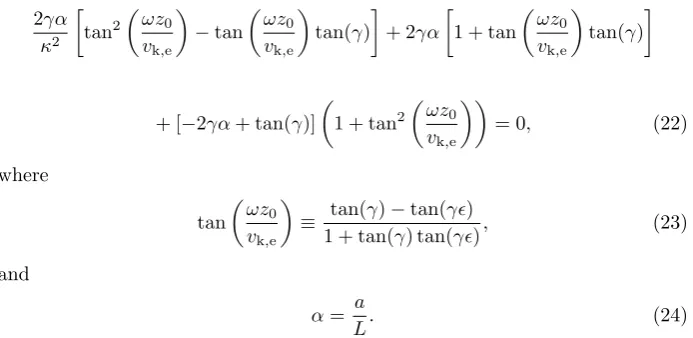
where z0 is the center of the step function anda is half the length of the step. Performing a similar analysis to Section 3, the dispersion relationship for this density profile can be written as

2γα κ2

tan2

ωz0 vk,e

−tan

ωz0 vk,e

tan(γ)

+ 2γα

1 + tan

ωz0 vk,e

tan(γ)

+ [−2γα+ tan(γ)]

1 + tan2

_ωz0

vk,e

= 0, (22)

where

tan

ωz0 vk,e

≡ tan(γ)−tan(γǫ)

1 + tan(γ) tan(γǫ), (23)

and

α= a

L. (24)

As we define the bead such that it is small, thereforea≪L, it is simple to note thatα≪1. This is consistent with assumptions made in other analytical works (e.g., D´ıaz, Oliver, and Ballester, 2010).

Continuing the analysis as in Section 3, we are able to expressγas

γn=nπ+

2n3_π3_α(κ2_−1)ǫ2

2n2_π2_αǫ(κ2_{−1)(1−3ǫ) +κ}2_{(1 +n}2_π2_ǫ2₎. (25)

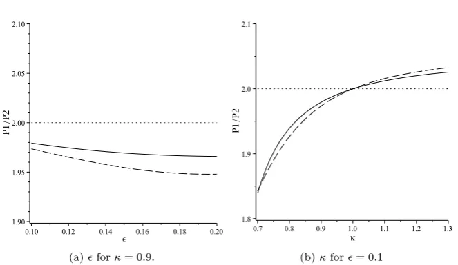
Figure 3 shows the period ratio using Equations (22) and (25) for the numerical and analytical solutions, respectively. As in Figure 2, we see a reasonably good agreement between the two solutions. For this plot, the newly defined length of the bead to the length of the loop ratio is held fixed at α= 0.1. Recalling the geometry of the problem (Figure 1),α= 0.1 creates the limitǫ >0.1.Intuitively, varying α will give different limits for ǫ. Once again we see that if κ <1, the ratio of the period of the harmonics drops below two (Figure 3b),i.e., the period ratio of a homogeneous oscillating loop. This finding agrees with both intuition and with observational evidence which suggest that heavy plasma propagating along coronal loops may influence each harmonic individually.

(a)ǫforκ= 0.9. (b)κforǫ= 0.1

Figure 3. Equivalent to Figure 2 for Equation (25).

5. Bead Propagation along Loop

Now, it is possible to add a time-dependence of the background state, represent-ing a gas plug flowrepresent-ing along the magnetic field lines (or a bead movrepresent-ing along a string). It is assumed that the initial density profile of the bead is close to the end of the loop as in Section 4, before advancing along the loop. This can be written concisely as

ρ(z, t) =

ρe z∈[0, z0+v0(z)t−a]∪[z0+v0(z)t+a, L];

ρb z∈[z0+v0(z)t−a, z0+v0(z)t+a], (26)

where t is time and v0(z) is the flow velocity of the bead. We take the initial point of the bead close toz0=L(and so ǫ≪1) and consider a constant speed of advancement in the negativez direction, that is v0(z)≡v0, v0<0. We now use the WKB method (see Bender and Orszag (1978) for more information on this technique) to solve the governing equation [Equation (1)] for the dynamic density profile. Application of the WKB method requires that the characteristic time of density changes should be small compared to the period of oscillations. This implies

δ≡ v0

L (27)

is small or |δt| ≪1. This assumption is reasonable when compared to observa-tions of flows (Ruderman (2010) suggested a reasonable limit to flow velocities should be approximately 100 km s−1_).

Continuity of the solution at the endpoints of the bead, as in Sections 3 and 4, allows us to obtain the dispersion relationship

2γαtan(γ)

tan

_ωz0

vk,e

+ Ω 1−tan

_ωz0

vk,e

Ω 1− 1 κ2

+(tan(γ)−2γα)

(

tan

ωz0 vk,e

+ Ω

2

+

1−tan

ωz0 vk,e

Ω

2)

+2γα

κ2

(

tan

_ωz0

vk,e

+ Ω

2

+κ2

1−tan

_ωz0

vk,e

Ω

2)

= 0, (28)

where

Ω = tan

ωv0t vk,e

. (29)

It is interesting to note that Equation (28) is equivalent to Equation (14) of Soler and Goossens (2011) who, however, investigated the properties of the fundamental harmonic of the kink mode within a solar prominence. Several key differences arise from those performed by Soler and Goossens (2011), including,

e.g., the ratio of the density of the bead and loop, as explained in Section 2. Now, by making some further simplifications, we seek to solve Equation (28) analytically, hence allowing the explicit calculation of the P1/P2 ratio for the specific density profile studied in this article.

Assuming thatL≫ |v0t|(i.e.at all modelled times, the distance travelled by bead is much less than L), in accordance with the WKB method, we find

Ω≈γδt. (30)

Applying Equation (30) to Equation (28) and using the techniques exploited in Sections 3 and 4, we obtain that

γn=nπ+

2n3_π3_α(κ2_{−1)(ǫ−δt)}2

2n2_π2_α(κ2_{−1)[δt(6ǫ−δt−1) +ǫ(1−3ǫ)] +κ}2_f1, (31)

where

f1= 1 +n2π2δ2t2+n2π2ǫ2. (32)

Here, we make note of several key limits. If bulk flows are absent, v0 = 0, we recover Equation (25) as we expect. Forκ <1 andt increasing, the ratio of the first two harmonics deviates from two towards zero,i.e., as a bead which is heavier than the background loop moves through a thin tube, the ratio of the fundamental and first harmonics decreases. Forκ >1 andtincreasing, we find that the period ratio increases from two,i.e., a light bead travelling through a thin tube increases the value of the harmonic ratios. If |v0t| ≪L we find that

P1/P2≈2,i.e., a small bead travelling very slowly has little effect on the ratio of the periods of the first two harmonics, as we would expect.

Figure 4. (a) The deviation ofγnfromnπover time. (b) Ratio ofγnwith respect tonπover

time. Line styles and corresponding harmonic are as follows: Solid line forn=1; dashed line forn= 2 and dot-dashed line forn= 3.

that Figure 4(b) shows a non-linear deviation for the harmonics and appears, forn= 3, to approach a minimum over time.

The influence of bulk flows from the footpoints of a loop into the corona, on standing MHD oscillations, is potentially an important tool for explaining the deviation of the observed P1/P2 ratios from the idealised, uniform oscillating loop ratios of two. In this article, we have derived an analytical approximation for theP1/P2 ratio of a moving bead (analogous to a small propagating density structure), finding approximate expressions which match closely with observa-tions. It is interesting to note that, in the model presented here, the localised density enhancements do not need to propagate deeply into the corona to influ-ence the period of standing oscillations. Strong bulk motions at the photospheric footpoints of such loop structures could cause rapid decrease of theP1/P2 ratio. In the following section, we discuss the influence of density stratification on the anti-nodes of standing MHD waves applicable to solar atmospheric oscillations,

e.g., to a coronal loop, thereby, presenting a second quantifiable value modi-fied by a propagating density structure. Such study may open new avenues in spatio magneto-seismology, providing conditional constraints on coronal loop modelling.

6. Anti-Node Shift

Figure 5. The change of the first harmonic anti-node shift over time with respect to velocities: 10 km s−1 _{(dot-dashed line); 25 km s}−1 _{(dashed line); 50 km s}−1 _{(dotted line) and 100 km}

s−1_{. Other parameters areL= 150 Mm,ǫ= 0.1,κ= 0.9,n= 2 andα= 0.05.}

The anti-node shift is an observable trait of oscillations which can be used as a novel diagnostic tool to infer background plasma properties. Using the anti-node shift to investigate solar structures is still in its infancy; mainly because the spatial resolution of current solar instrumentation is just about at the sensitivity to search for and detect this effect in standing oscillations. It is not yet thoroughly expanded upon in the literature. Work such as we present here could become a valuable addition to this new and exciting technique.

We shall begin by noting that the position of the anti-nodes can be found by calculating

d

dz(zAN) = 0, (33)

where z = zAN is the positions of the anti-nodes. To calculate shift, one must first calculate the position of the anti-nodes for a homogeneous loop. We then assume weak stratificationρe≈ρbto find the position of the anti-nodes for the inhomogenous case. Once these are known, it is simple to subtract one from the other to derive the anti-node shift expressed as

∆zAN=

(2n−1)L

2

_π

γn

−1 n

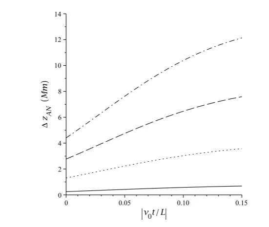
Figure 6. Variance of the anti-nodes over time forn= 2. Different lines correspond to different sizes ofαin our model, namely: 0.01 (solid line), 0.05 (dotted line), 0.1 (dashed line), and 0.15 (dot-dashed line). It is simple to see that larger beads cause larger shifts of the anti-nodes.

Substituting Equation (20) into Equation (34), it is easy to calculate

∆zAN=

(2n−1)L

2n

_3ǫ3_n2_π2_(1−κ2_{) + 3κ}2_{(1 +ǫ}2_n2_π2₎

2ǫ3_n2_π2_(1−κ2_{) + 3κ}2_{(1 +ǫ}2_n2_π2₎−1

(35)

for the single-density-discontinuity case. Note that if κ = 1, i.e., there is no density jump, we retrieve ∆zAN = 0. Therefore, no change in the anti-nodes, as we would expect. Here, it is found that if there is a stronger contrast in the densities (i.e.|κ| increases) then a higher anti-node shift would be manifested. Substituting characteristic values applicable to coronal loops,e.g.,L= 150 Mm,

ǫ = 0.1, κ = 0.9, and n = 2 (i.e., the first harmonic) into Equation (35), we find ∆zAN= 0.248 Mm which is a relatively small deviation of node movement over the length of the loop. This would be harder to measure with the currently available instrumental limit, though with improving technology it is anticipated that such measurements should be carried out in the near future.

Next, let us derive the anti-node shift for the step-density. After some algebra we find

∆zAN=

(2n−1)L

2n

_2n2_π2_αǫ(κ2_{−1)(3ǫ−1)−κ}2_{(1 +n}2_π2_ǫ2₎

2n2_π2_αǫ(κ2_{−1)(2ǫ−1)−κ}2_{(1 +n}2_π2_ǫ2₎−1

. (36)

0.789 Mm. This is a significant estimated deviation from the unperturbed anti-nodes, even close to the spatial resolution of theAtmospheric Imaging Assembly

onboard the Solar Dynamics Observatory spacecraft (SDO/AIA) instrument, implying that observations of these shifts could be possible. We would strongly encourage the community to pursue observational studies into spatio magneto-seismology.

Finally, we determine the anti-node shift of a thin loop over time when a bead is propagating away from its footpoint. This can be written as:

∆zAN=

(2n−1)L

2n

_2n2_π2_α(κ2_−1)f2+κ2_f1

2n2_π2_α(κ2_{−1) [f2+ (ǫ−δt)}2_{] +κ}2_f1 −1

(37)

where

f2=δt(6ǫ−δt−1) +ǫ(1−3ǫ) (38)

andf1is as described in Equation (32).

In Figure 5, we plot the anti-node shift over time from t = 0 (taken as the conditions stated after Equation (36) and varying α, the ratio of half of the length of the bead to the length of the loop). The plot beautifully agrees with the intuitive result, that faster propagating bead will cause larger anti-node shift. Next, in Figure 6, anti-node shifts are plotted for different flowing bead lengths. It is found that small beads cause relatively small anti-node shifts (less than 2 Mm). However, even for values such as α= 0.15, anti-node shifts of around 12 Mm can be found. As the bead propagates away from the footpoint of the loop, it is found that the deviation from the unperturbed anti-nodes increases. Given that the pixel size of the SDO/AIA instrument is fixed at 0.6′′_{, we note that} values such as 2−12 Mm may be easily observable with current techniques.

7. Discussion and Conclusions

In this article, we have presented both an analytical approximation for the period ratio of transversally oscillating coronal loops, with different density profiles representing a density jump, a static bead and a moving bead. An estimate of the accompanying anti-node shift was found. These two quantifiable, and complimentary, physical parameters for transverse standing oscillations could provide clear insight into the background characteristics of magnetic loops in the solar atmosphere. The model discussed in this work encompasses localised bulk flows from loop footpoints into higher regions of the atmosphere. We find that these localised density enhancements can have a large and measurable influence by both modifying theP1/P2 period ratios and causing anti-node shifts within flux tube structures.

modification of theP1/P2 ratio to a value less than its canonical value. Although it is not directly studied in this article, it is interesting to note here that the Equations derived here also apply to beadslighterthan the background density of the flux tube and show an increase of theP1/P2 period ratio from two.

The model studied in this article was dependent on a number of parameters, specifically, the ratio of the kink speed of tube sections andǫ, the dimensionless position of the bead along the loop. Analytical solutions were obtained such that

ǫ ≪1,i.e., a jet flow propagating from the photosphere or chromosphere into the corona (as observed by, e.g., Ofman and Wang, 2008). It is important to note that the background density of the loop studied in this model includes no stratification and, therefore, presents a simplistic example.

Wave propagation in a continuously stratifiied magnetic atmosphere, rather than a flux tube, has been studied extensively. Vertical and oblique magnetic fields were investigated by, e.g., Ferraro and Plumpton (1958) and Leroy and Bel (1979), respectively. Campos (1987) found that the P1/P2 ratio for standing Alfv´en waves in an isothermal atmosphere (where the layer is larger than the atmospheric scale height) is given byj2/j1= 2.25, wherejn is then-th root of the Bessel function J0. This increase from 2 for Alfv´en waves is not in direct disagreement with our results for kink waves in a thin flux tube as each case neglects a different feature of a more complex, and realistic, model of a flux tube with continuous density stratification and flows.

TheP1/P2 period ratio was also derived as a function of time for a moving bead through a loop. It was found that larger values of n cause quicker and larger divergence from the typical period of nπ leading to a decreasing period ratio initially. This suggests that the largest divergence from the expectedP1/P2 period ratio for a homogeneous bounded flux tube occurs when the bead is in a spatial position such that|v0t/L| →0.2. However, due to our approximation assumptions, we are unable to verify this analytically. We conclude that density stratification can play an important role in the deviation of the P1/P2 ratio from two. Future studies should be undertaken with the aim of discussing more advanced, and applicable, density profiles (such as a bead flowing through a non-homogeneous background loop).

Finally, anti-node shifts generated through density stratification were dis-cussed. It was found that, as the bead propagates away from the end of the loop, the anti-node shifts increase in general. Overall, we suggest that localised bulk flows within loop structures could be an important factor in explaining observed localised anti-node shifts.

References

Andries, J., Arregui, I., Goossens, M.: 2005, Determination of the coronal density stratification from the observation of harmonic coronal loop oscillations. Astrophys. J. Lett.624, L57. Andries, J., van Doorsselaere, T., Roberts, B., Verth, G., Verwichte, E., Erd´elyi, R.: 2009,

Coronal seismology by means of kink oscillation overtones. Space Sci. Rev.149, 3. Aschwanden, M.J., Fletcher, L., Schrijver, C.J., Alexander, D.: 1999, Coronal loop oscillations

observed with the Transition Region and Coronal Explorer.Astrophys. J.520, 880. Bender, C.M., Orszag, S.A.: 1978, Advanced Mathematical Methods for Scientists and

Engineers: McGraw Hill, New York, 484.

Berghmans, D., Clette, F.: 1999, Active region EUV transient brightenings - First results by EIT of SOHO JOP80.Solar Phys.186, 207.

Campos, L.M.B.C.: 1986, On umbral oscillations as a sunspot diagnostic. In: Gough, D.O. (ed.), Seismology of the Sun and the Distant Stars, NATO ASI Series C 169, 293. Campos, L.M.B.C.: 1987, On waves in gases. Part II: Interaction of sound with magnetic and

internal modes.Rev. Mod. Phys.59, 363.

De Moortel, I.: 2009, Longitudinal waves in coronal loops. Space Sci. Rev.149, 65.

De Moortel, I., Brady, C.S.: 2007, Observation of higher harmonic coronal loop oscillations.

Astrophys. J.664, 1210.

Deforest, C.E., Gurman, J.B.: 1998, Observation of quasi-periodic compressive waves in solar polar plumes. Astrophys. J. Lett.501, L217.

D´ıaz, A.J., Oliver, R., Ballester, J.L.: 2010, Prominence thread seismology using theP1/2P2

ratio. Astrophys. J.725, 1742.

Dymova, M.V., Ruderman, M.S.: 2005, Non-axisymmetric oscillations of thin prominence fibrils.Solar Phys.229, 79.

Edwin, P.M., Roberts, B.: 1983, Wave propagation in a magnetic cylinder.Solar Phys. 88, 179.

Erd´elyi, R.: 2006, In:Fletcher, K., Thompson, M. (eds.) Proceedings of SOHO 18/GONG 2006/HELAS I, Beyond the Spherical Sun, ESA SP-624, p.15.1 (on CDROM).

Erd´elyi, R., Taroyan, Y.: 2008, Hinode EUV spectroscopic observations of coronal oscillations.

Astron. Astrophys.489, L49.

Erd´elyi, R., Verth, G.: 2007, The effect of density stratification on the amplitude profile of transversal coronal loop oscillations. Astron. Astrophys.462, 743.

Ferraro, C.A., Plumpton, C.: 1958, Hydromagnetic waves in a horizontally Stratified atmo-sphere. V. Astrophys. J.127, 459.

Jess, D.B., Mathioudakis, M., Erd´elyi, R., Verth, G., McAteer, R.T.J., Keenan, F.P.: 2008, Dis-covery of spatial periodicities in a coronal loop using automated edge-tracking algorithms.

Astrophys. J.680, 1523.

Jess, D.B., Mathioudakis, M., Erd´elyi, R., Crockett, P.J., Keenan, F.P., Christian, D.J.: 2009, Alfv´en waves in the lower solar atmosphere.Science 323, 1582.

Kopp, R.A., Poletto, G., Noci, G., Bruner, M.: 1985, Analysis of loop flows observed on 27 March, 1980 by the UVSP instrument during the Solar Maximum Mission.Solar Phys.

98, 91.

Leroy, B., Bel, N.: 1979, Propagation of waves in an atmosphere in the presence of a magnetic field. I - The method. Astron. Astrophys.78, 129.

Mathioudakis, M., Jess, D.B., Erd´elyi, R.: 2012, Alfv´en waves in the solar atmosphere. Space Sci. Rev., 94. doi:10.1007/s11214-012-9944-7.

Morton, R.J., Erd´elyi, R.: 2009, Transverse oscillations of a cooling coronal loop. Astrophys. J.707, 750.

Nakariakov, V.M., Ofman, L.: 2001, Determination of the coronal magnetic field by coronal loop oscillations. Astron. Astrophys.372, L53.

Ofman, L., Wang, T.J.: 2008, Hinode observations of transverse waves with flows in coronal loops. Astron. Astrophys.482, L9.

O’Shea, E., Srivastava, A.K., Doyle, J.G., Banerjee, D.: 2007, Evidence for wave harmonics in cool loops. Astron. Astrophys.473, L13.

Roberts, B.: 2000, Waves and oscillations in the corona (invited review).Solar Phys.193, 139. Roberts, B., Edwin, P.M., Benz, A.O.: 1984, On coronal oscillations.Astrophys. J.279, 857. Rosenberg, H.: 1970, Evidence for MHD pulsations in the solar corona. Astron. Astrophys.9,

159.

Ruderman, M.S., Erd´elyi, R.: 2009, Transverse oscillations of coronal loops. Space Sci. Rev.

149, 199.

Soler, R., Goossens, M.: 2011, Kink oscillations of flowing threads in solar prominences. Astron. Astrophys.531, A167.

Soler, R., Ruderman, M.S., Goossens, M.: 2012, Damped kink oscillations of flowing promi-nence threads. Astron. Astrophys.546, A82.

Srivastava, A.K., Zaqarashvili, T.V., Uddin, W., Dwivedi, B.N., Kumar, P.: 2008, Observation of multiple sausage oscillations in cool post-flare loop. Mon. Not. Roy. Astron. Soc.388, 1899.

Taroyan, Y., Erd´elyi, R.: 2009, Heating diagnostics with MHD waves. Space Sci. Rev.149, 229.

Uchida, Y.: 1970, Diagnosis of coronal magnetic structure by flare-associated hydromagnetic disturbances. Publ. Astron. Soc. Japan22, 341.

Van Doorsselaere, T., Nakariakov, V.M., Verwichte, E.: 2007, Coronal loop seismology using multiple transverse loop oscillation harmonics. Astron. Astrophys.473, 959.

Verth, G., Erd´elyi, R.: 2008, Effect of longitudinal magnetic and density inhomogeneity on transversal coronal loop oscillations. Astron. Astrophys.486, 1015.

Verth, G., Erd´elyi, R., Jess, D.B.: 2008, Refined magnetoseismological technique for the solar corona. Astrophys. J. Lett.687, L45.

Verth, G., Van Doorsselaere, T., Erd´elyi, R., Goossens, M.: 2007, Spatial magneto-seismology: Effect of density stratification on the first harmonic amplitude profile of transversal coronal loop oscillations. Astron. Astrophys.475, 341.

Verwichte, E., Nakariakov, V.M., Ofman, L., Deluca, E.E.: 2004, Characteristics of transverse oscillations in a coronal loop arcade.Solar Phys.223, 77.

Wang, T.: 2011, Standing slow-mode waves in hot coronal loops: Observations, modeling, and coronal seismology. Space Sci. Rev.158, 397.