mass M dwarf in the pre-cataclysmic binary NN Serpentis
.
White Rose Research Online URL for this paper:
http://eprints.whiterose.ac.uk/108466/
Version: Accepted Version
Article:
Parsons, S. G., Marsh, T. R., Copperwheat, C. M. et al. (4 more authors) (2010) Precise
mass and radius values for the white dwarf and low mass M dwarf in the pre-cataclysmic
binary NN Serpentis. Monthly Notices of the Royal Astronomical Society , 402 (4). pp.
2591-2608. ISSN 0035-8711
https://doi.org/10.1111/j.1365-2966.2009.16072.x
[email protected]
https://eprints.whiterose.ac.uk/
Reuse
Unless indicated otherwise, fulltext items are protected by copyright with all rights reserved. The copyright
exception in section 29 of the Copyright, Designs and Patents Act 1988 allows the making of a single copy
solely for the purpose of non-commercial research or private study within the limits of fair dealing. The
publisher or other rights-holder may allow further reproduction and re-use of this version - refer to the White
Rose Research Online record for this item. Where records identify the publisher as the copyright holder,
users can verify any specific terms of use on the publisher’s website.
Takedown
If you consider content in White Rose Research Online to be in breach of UK law, please notify us by
arXiv:0909.4307v2 [astro-ph.SR] 19 Nov 2009
Mon. Not. R. Astron. Soc.000, 1–20 (2009) Printed 19 November 2009 (MN LATEX style file v2.2)
Precise mass and radius values for the white dwarf and low
mass M dwarf in the pre-cataclysmic binary NN Serpentis
S. G. Parsons
1⋆, T. R. Marsh
1, C. M. Copperwheat
1, V. S. Dhillon
2,
S. P. Littlefair
2, B. T. G¨
ansicke
1and R. Hickman
11Department of Physics, University of Warwick, Coventry, CV4 7AL
2Department of Physics and Astronomy, University of Sheffield, Sheffield S3 7RH
Accepted 2009 November 18. Received 2009 November 17; in original form 2009 September 22
ABSTRACT
Using the high resolution Ultraviolet and Visual Echelle Spectrograph (UVES) mounted on the Very Large Telescope (VLT) in combination with photometry from the high-speed CCD camera ULTRACAM, we derive precise system parameters for the pre-cataclysmic binary, NN Ser. A model fit to the ULTRACAM light curves gives the orbital inclination as i= 89.6◦±0.2◦and the scaled radii,RWD/aandRsec/a. Analysis
of the HeII 4686˚A absorption line gives a radial velocity amplitude for the white dwarf ofKWD= 62.3±1.9 km s−1. We find that the irradiation-induced emission lines from
the surface of the secondary star give a range of observed radial velocity amplitudes due to differences in optical depths in the lines. We correct these values to the centre of mass of the secondary star by computing line profiles from the irradiated face of the secondary star. We determine a radial velocity ofKsec= 301±3 km s−
1
, with an error dominated by the systematic effects of the model. This leads to a binary separation of a = 0.934±0.009 R⊙, radii of RWD= 0.0211±0.0002 R⊙and Rsec= 0.149±0.002 R⊙ and masses of MWD= 0.535±0.012 M⊙ and Msec= 0.111±0.004 M⊙. The masses
and radii of both components of NN Ser were measured independently of any mass-radius relation. For the white dwarf, the measured mass, mass-radius and temperature show excellent agreement with a ‘thick’ hydrogen layer of fractional mass MH/MWD= 10−
4
. The measured radius of the secondary star is 10% larger than predicted by models, however, correcting for irradiation accounts for most of this inconsistency, hence the secondary star in NN Ser is one of the first precisely measured very low mass objects (M .0.3 M⊙) to show good agreement with models. ULTRACAMr’,i’ andz’ pho-tometry taken during the primary eclipse determines the colours of the secondary star
as (r’-i’)sec = 1.4±0.1 and (i’-z’)sec= 0.8±0.1 which corresponds to a spectral type
of M4±0.5. This is consistent with the derived mass, demonstrating that there is no detectable heating of the unirradiated face, despite intercepting radiative energy from the white dwarf which exceeds its own luminosity by over a factor of 20.
Key words: binaries: eclipsing – stars: fundamental parameters – stars: late-type – white dwarfs – stars: individual: NN Ser
1 INTRODUCTION
Precise measurements of masses and radii are of fundamen-tal importance to the theory of stellar structure and evolu-tion. Mass-radius relations are routinely used to estimate the masses and radii of stars and stellar remnants, such as white dwarfs. Additionally, the mass-radius relation for white dwarfs has played an important role in estimating the distance to globular clusters (Renzini et al. 1996) and the
determination of the age of the galactic disk (Wood 1992). However, the empirical basis for this relation is uncertain (Schmidt 1996) as there are very few circumstances where both the mass and radius of a white dwarf can be measured independently and with precision.
white dwarfs are indirect, relying on complex model atmo-sphere predictions. They were able to support the mass-radius relation on observational grounds more firmly, though they explain that parallax remains a dominant source of un-certainty, particularly for CPM systems. Improvements in our knowledge of the masses and radii of white dwarfs re-quires additional measurements. One situation where this is possible is in close binary systems. In these cases, masses can be determined from the orbital parameters and radii from light-curve analysis. Of particular usefulness in this re-gard are eclipsing post-common envelope binaries (PCEBs). The binary nature of these objects helps determine accurate parameters and, since they are detached, they lack the com-plications associated with interacting systems such as cat-aclysmic variables. The inclination of eclipsing systems can be constrained much more strongly than for non-eclipsing systems. Furthermore, the distance to the system does not have to be known, removing the uncertainty due to parallax. An additional benefit of studying PCEBs is that under favourable circumstances, not only are the white dwarf’s mass and radius determined independently of any model, so too are the mass and radius of its companion. These are often low mass late-type stars, for which there are few precise mass and radius measurements. There is disagree-ment between models and observations of low mass stars; the models tend to under predict the radii by as much as 20-30% (L´opez-Morales 2007). Hence detailed studies of PCEBs can lead to improved statistics for both white dwarfs and low mass stars. Furthermore, models of low mass stars are important for understanding the late evolution of mass transferring binaries such as cataclysmic variables (Littlefair et al. 2008).
[image:3.612.306.547.125.247.2]The PCEB NN Ser (PG 1550+131) is a low mass bi-nary system consisting of a hot white dwarf primary and a cool M dwarf secondary. It was discovered in the Palomar Green Survey (Green et al. 1982) and first studied in de-tail by Haefner (1989) who presented an optical light curve showing the appearance of a strong heating effect and very deep eclipses (>4.8mag at λ ∼ 6500 ˚A). Haefner identi-fied the system as a pre-cataclysmic binary with an orbital period of 0.13d. The system parameters were first derived by Wood & Marsh (1991) using low-resolution ultra-violet spectra then refined by Catalan et al. (1994) using higher resolution optical spectroscopy. Haefner et al. (2004) fur-ther constrained the system parameters using the FORS instrument at the Very Large Telescope (VLT) in combina-tion with high-speed photometry and phase-resolved spec-troscopy. However, they did not detect the secondary eclipse leading them to underestimate the binary inclination and hence overestimate the radius and ultimately the mass of the secondary star. They were also unable to directly mea-sure the radial velocity amplitude of the white dwarf and were forced to rely upon a mass-radius relation for the sec-ondary star. Recently, Brinkworth et al. (2006) performed high time resolution photometry of NN Ser using the high-speed CCD camera ULTRACAM mounted on the William Herschel Telescope (WHT). They detected the secondary eclipse leading to a better constraint on the inclination, and also detected a decrease in the orbital period which they determined was due either to the presence of a third body, or to a genuine angular momentum loss. Since NN Ser be-longs to the group of PCEBs which is representative for the
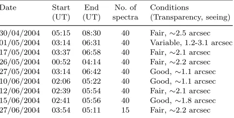
Table 1.Journal of VLT/UVES spectroscopic observations.
Date Start End No. of Conditions
(UT) (UT) spectra (Transparency, seeing)
30/04/2004 05:15 08:30 40 Fair,∼2.5 arcsec 01/05/2004 03:14 06:31 40 Variable, 1.2-3.1 arcsec 17/05/2004 03:37 06:58 40 Fair,∼2.1 arcsec 26/05/2004 00:52 04:14 40 Fair,∼2.2 arcsec 27/05/2004 03:14 06:42 40 Good,∼1.1 arcsec 10/06/2004 02:06 05:22 40 Good,∼1.1 arcsec 12/06/2004 02:39 05:54 40 Fair,∼2.1 arcsec 15/06/2004 02:41 05:56 40 Good,∼1.8 arcsec 27/06/2004 03:54 05:11 15 Fair,∼2.2 arcsec
progenitors of the current cataclysmic variable (CV) popu-lation (Schreiber & G¨ansicke 2003), the system parameters are important from both an evolutionary point of view as well as providing independent measurements of the masses and radii of the system components.
In this paper we present high resolution VLT/UVES spectra and high time resolution ULTRACAM photometry of NN Ser. We use these to determine the system parameters directly and independently of any mass-radius relations. We compare our results with models of white dwarfs and low mass stars.
2 OBSERVATIONS AND THEIR REDUCTION 2.1 Spectroscopy
Precice mass and radius values for both components of the pre-CV NN Ser
3
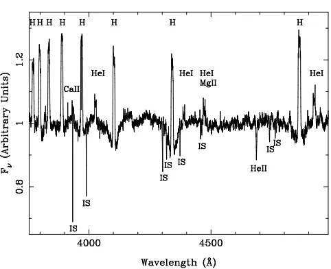
Figure 1.Averaged, normalised UVES blue arm spectrum with the blaze removed. IS corresponds to interstellar absorption fea-tures. The discontinuity at∼4150˚A and the emission-like feature at∼4820˚A are most likely instrumental features or artifacts of the UVES reduction pipeline as they are seen in all 335 spectra.
phase of each spectrum was calculated using the ephemeris of Brinkworth et al. (2006).
The spectral features seen are similar to those reported by Catalan et al. (1994) and Haefner et al. (2004): Balmer lines, which appear as either emission or absorption depend-ing upon the phase, HeI and CaII emission lines and HeII 4686˚A in absorption. The Paschen series is also seen in emission in the far red. In addition, MgII 4481˚A emission is seen as well as a number of fainter MgII emission lines beyond 7800˚A . Weak FeI emission lines are seen through-out the spectrum and faint CI emission is seen beyond 8300˚A (see Table 4 for a full list of identified emission lines). The strength of all the emission lines is phase-dependent, peaking at phase 0.5, when the heated face of the secondary star is in full view, then disappearing around the primary eclipse. Several sharp absorption features are observed not to move over the orbital period, these are interstellar ab-sorption features and include interstellar CaII abab-sorption.
2.2 Blaze Removal
An echelle grating produces a spectrum that drops as one moves away from the blaze peak, this is known as the blaze function. After reduction a residual ripple pattern was visi-ble in the blue spectra corresponding to the blaze function. This was approximately removed by fitting with a sinusoid of the form
B(λ) = a0+a1sin(2πφ) +a2λsin(2πφ) (1) +a3cos(2πφ) +a4λcos(2πφ).
The phase (φ) was calculated by identifying the central wavelength of each echelle order. The line table produced using the ESORex recipe uves cal wavecal provided this in-formation. Then using the relation
λn(O−n) =c, (2)
wherecandOare constants andλnis the central wavelength
of ordern, gives us the phase. We find values ofO= 125 and
c= 465700, which are similar for all the spectra. Therefore the phase of the ripple is
φ= 125−465700 λ .
Since the phase is now known, Equation 1 reduces to a sim-ple linear fit. Figure 1 is a normalised average of all the UVES blue arm spectra with the blaze removed. Since this is only a simple fit some residual pattern does remain after division by the blaze function but overall the effect is greatly reduced.
2.3 Photometry
The data presented here were collected with the high speed CCD camera ULTRACAM (Dhillon et al. 2007), mounted as a visitor instrument on the 4.2m William Herschel Tele-scope (WHT) and on the VLT in June 2007. A total of ten observations were made in 2002 and 2003, and these data were supplemented with observations made at a rate of∼1 – 2 a year up until 2008. ULTRACAM is a triple beam cam-era and most of our observations were taken simultaneously through the SDSSu’,g’ and i’ filters. In a number of in-stances anr’ filter was used in place ofi’; this was mainly for scheduling reasons. Additionally, az’ filter was used in place ofi’for one night in 2003.
A complete log of the observations is given in Table 2. We windowed the CCD in order to achieve an exposure time of 2 – 3s, which we varied to account for the conditions. The dead time was∼25ms.
All of these data were reduced using the ULTRACAM pipeline software. Debiassing, flatfielding and sky back-ground subtraction were performed in the standard way. The source flux was determined with aperture photometry using a variable aperture, whereby the radius of the aperture is scaled according to the FWHM. Variations in observing con-ditions were accounted for by determining the flux relative to a comparison star in the field of view. There were a num-ber of additional stars in the field which we used to check the stability of our comparison. For the flux calibration we determined atmospheric extinction coefficients in theu’,g’
andr’bands and subsequently determined the absolute flux of our targets using observations of standard stars (from Smith et al. 2002) taken in twilight. We use this calibra-tion for our determinacalibra-tions of the apparent magnitudes of the two sources, although we present all light curves in flux units determined using the conversion given in Smith et al. (2002). Using our absorption coefficients we extrapolate all fluxes to an airmass of 0. The systematic error introduced by our flux calibration is < 0.1 mag in all bands. For all data we convert the MJD times to the barycentric dynami-cal timesdynami-cale, corrected to the solar system barycentre.
differ-Table 2.ULTRACAM observations of NN Ser. The primary eclipse occurs at phase 1, 2 etc.
Date Filters Telescope UT UT Average Phase Conditions
start end exp time (s) range (Transparency, seeing)
[image:5.612.86.496.123.327.2]17/05/2002 u’g’r’ WHT 21:54:40 02:07:54 2.4 0.85–2.13 Good,∼1.2 arcsec 18/05/2002 u’g’r’ WHT 21:21:20 02:13:17 3.9 0.39–1.23 Variable, 1.2-2.4 arcsec 19/05/2002 u’g’r’ WHT 23:58:22 00:50:52 2.0 0.93–1.10 Fair,∼2 arcsec 20/05/2002 u’g’r’ WHT 00:58:23 01:57:18 2.3 0.86–1.14 Fair,∼2 arcsec 19/05/2003 u’g’z’ WHT 22:25:33 01:02:25 6.7 0.47–1.12 Variable, 1.5-3 arcsec 21/05/2003 u’g’i’ WHT 00:29:00 04:27:32 1.9 0.32–0.59 Excellent,∼1 arcsec 22/05/2003 u’g’i’ WHT 03:24:57 03:50:40 2.0 0.36–0.08 Excellent,<1 arcsec 24/05/2003 u’g’i’ WHT 22:58:55 23:33:49 2.0 0.90–0.08 Good,∼1.2 arcsec 25/05/2003 u’g’i’ WHT 01:29:45 02:15:58 2.0 0.39–0.64 Excellent,∼1 arcsec 03/05/2004 u’g’i’ WHT 22:13:44 05:43:11 2.5 0.37–2.27 Variable, 1.2-3.2 arcsec 04/05/2004 u’g’i’ WHT 23:18:46 23:56:59 2.5 0.91–0.61 Variable, 1.2-3 arcsec 09/03/2006 u’g’r’ WHT 01:02:34 06:46:49 2.0 0.91–2.70 Variable, 1.2-3 arcsec 10/03/2006 u’g’r’ WHT 05:01:13 05:50:14 2.0 0.85–1.11 Excellent,<1 arcsec 09/06/2007 u’g’i’ VLT 04:59:25 05:46:18 0.9 0.40–0.61 Excellent,∼1 arcsec 16/06/2007 u’g’i’ VLT 03:57:48 04:54:39 2.0 0.86–1.15 Good,∼1.2 arcsec 17/06/2007 u’g’i’ VLT 01:50:16 02:38:09 1.0 0.86–1.11 Excellent,<1 arcsec 07/08/2008 u’g’r’ WHT 23:41:29 00:22:46 2.8 0.87–1.07 Excellent,<1 arcsec
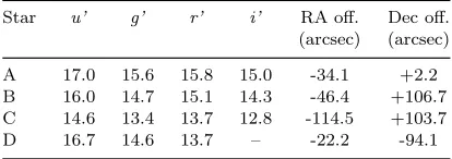
Table 3.Comparison star magnitudes and positional offsets from NN Ser. There were noi’ band observations of star D. The mag-nitudes for the white dwarf in NN Ser are shown in Table 6.
Star u’ g’ r’ i’ RA off. Dec off. (arcsec) (arcsec)
A 17.0 15.6 15.8 15.0 -34.1 +2.2 B 16.0 14.7 15.1 14.3 -46.4 +106.7 C 14.6 13.4 13.7 12.8 -114.5 +103.7 D 16.7 14.6 13.7 – -22.2 -94.1
ences by using the comparison star observations. A first-order polynomial was fit to the comparison star photometry in order to determine the comparison star’s colours (mag-nitudes listed in Table 3). The colour of the white dwarf in NN Ser was calculated by fitting a zeroth-order polynomial to the flat regions around the primary eclipse with a cor-rection made in ther’ andi’ bands for the secondary stars contribution (the contribution of the secondary star in the
u’ and g’ bands around the primary eclipse is negligible). The colour dependant difference in extinction coefficients for the comparison star and NN Ser were then calculated from a theoretical extinction vs. colour plot1. The additional ex-tinction correction for NN Ser for each night is then
102.51 (kN−kC)X, (3)
where kN is the extinction coefficient for NN Ser, kC is the
extinction coefficient for the comparison and X is the air-mass. The value ofkN−kCfor each band was similar for all
the comparisons used. In the u’ filterkN−kC ∼0.03, for
theg’bandkN−kC∼0.02, for ther’bandkN−kC∼0.002
and for thei’ bandkN−kC∼0.0005.
The flux-calibrated, extinction-corrected light curves for each filter were phase binned using the ephemeris of Brinkworth et al. (2006). Data within each phase bin were
1 theoretical extinction vs. colour plots for ULTRACAM are
[image:5.612.307.547.279.576.2]available at http://garagos.net/dev/ultracam/filters
Figure 2.Digital Sky Survey finding chart (POSS II,blue) for NN Ser. Comparison stars are marked.
averaged using inverse variance weights whereby data with smaller errors are given larger weightings. Smaller bins were used around both the eclipses. The result of this is a set of high signal-to-noise light curves for NN Ser (one for each filter).
2.4 Flux Calibration
[image:5.612.58.265.386.459.2]Precice mass and radius values for both components of the pre-CV NN Ser
5
[image:6.612.43.285.439.630.2]Figure 3.Averaged spectra from the blue, lower and upper red CCD chips with ULTRACAM filter response curves. The spectra were not telluric corrected. Thedotted line is the filter profile based on theg’ filter used to flux calibrate the UVES blue CCD spectra since theg’ filter doesn’t cover the same spectra range.
Figure 4.Sine curve fit for the HeII 4686˚A absorption line fitted with a straight line and a Gaussian. The measured radial velocity amplitude for the primary is 62.3±1.9 km s−1.
8670–10400˚A ) along with ULTRACAM response curves for each filter. A simple model was fitted to the ULTRACAMg’
andi’ light curves (see Section 4.1 for details of the model fitting). The aim of this model was to reproduce the light curve as closely as possible. The model was then used to predict the flux at the times of each of the UVES observa-tions (NN Ser shows no stochastic variaobserva-tions or flaring de-spite the rapidly rotating secondary star). Since thei’filter
Figure 5.Sine curve fit to the Balmer absorption features near the primary eclipse over-plotted with the radial velocity ampli-tude of the primary calculated using the HeII line, the deviations away from the eclipse are caused by emission from the secondary star, hence those spectra within thedashedlines contain no emis-sion from the secondary star.
[image:6.612.304.543.440.625.2]Figure 6. Normalised white dwarf spectrum with an over-plotted T = 57000K, logg = 7.5 white dwarf model spectrum including homogeneously mixed helium (NHe= 4×10⁻⁴ by number). IS corresponds to interstellar absorption features.
of theg’filter, while avoiding Hβto prevent its biassing the results.
The average flux of each spectrum was calculated within these filters then compared to the model light curve value for that phase. The spectrum was then multiplied by an ap-propriate constant to match these values up. Since there is only one z’ ULTRACAM light curve which, due to condi-tions, was fairly poor, it was not used to flux calibrate the UVES upper red CCD spectra even though it covers a simi-lar spectra range. Rather, thei’ model was extrapolated to the longer wavelength range.
3 RESULTS
3.1 The White Dwarf ’s Spectrum
In order to recover the white dwarf’s spectrum, its radial velocity amplitude must be calculated. Due to the broad nature of the Balmer absorption features and the contam-ination by emission from the secondary star, we concluded that using the Balmer absorption lines to calculate the ra-dial velocity amplitude of the white dwarf would be likely to give an incorrect result. Fortunately, the narrower HeII 4686˚A absorption line is seen in absorption at all phases and no HeII emission is seen at any time throughout the spectra. In addition, there are no nearby features around the HeII 4686˚A line making it a good feature to use to cal-culate the radial velocity amplitude of the white dwarf; it is indeed the only clean feature from the white dwarf that we could identify. We fit the line using a combination of a straight line plus a Gaussian. We use this to calculate a radial velocity amplitude for the white dwarf.
Figure 4 shows the fit to the HeII 4686˚A velocities. The radial velocity amplitude found is 62.3±1.9 km s−1
significantly smaller than the value of 80.4±4.1 km s−1 cal-culated indirectly by Haefner et al. (2004) from their light curve analysis as they relied upon a mass-radius relation for the secondary star. The difference is due to their overesti-mation of the mass of the secondary star by roughly 30%.
Just before and after the primary eclipse the repro-cessed light from the secondary star is not yet visible, hence spectra taken at these phases contain just the white dwarf’s features. More precise constraints on this range can be made by studying the Balmer lines. The deep wide Balmer absorp-tion lines from the white dwarf are gradually filled in by the emission from the secondary star as the system moves away from the primary eclipse. Multiple Gaussians were fit to the Balmer absorption features, any deviation from this is due to emission from the secondary star which increases the mea-sured velocity amplitude of the lines. Figure 5 shows this fit along with the HeII 4686˚A radial velocity amplitude fit. No deviation is seen before phase∼ 0.12 and after phase
∼ 0.88 hence spectra taken between these phases contain spectral information on the white dwarf only (except those taken during the eclipse).
The spectra were shifted to the white dwarf’s frame us-ing the calculated radial velocity amplitude, then the spectra within the phase range quoted were averaged using weights for optimum signal-to-noise (ignoring those spectra taken during the eclipse). The result is the spectrum of the white dwarf component of NN Ser only, as shown in Figure 6. We match a homogeneously mixed hydrogen and helium atmo-sphere white dwarf model with a temperature of 57,000K
and logg= 7.5 to the white dwarf spectrum (also shown in Figure 6). A helium abundance of 4.0±0.5×10⁻⁴ by number is required to reproduce the measured equivalent width of the HeII line (0.25±0.02˚A). The result is in agreement with
Precice mass and radius values for both components of the pre-CV NN Ser
7
Figure 7. Trailed spectra of various lines. The white dwarf component has been subtracted. White represents a value of 0.0 in all trails. For the Balmer lines and the Paschen line, black represents a value of 2.0, for the other lines, black represents a value of 1.0. The subtraction of the white dwarf component creates a peak on the CaII trail due to the presence of interstellar absorption.
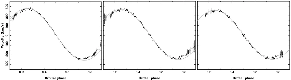
Figure 8.Sine curve fits for the Balmer lines (left), the three strongest He I lines (centre), and the MgII 4481˚A line (right). The lines were fit using a straight line and a Gaussian. The MgII 4481˚A line becomes too faint before phase 0.15 and after phase 0.85 to fit.
Stark broadening in the code we used to calculate the model (TLUSTY, Hubeny 1988, Hubeny & Lanz 1995). The white dwarf spectrum shows only Balmer and HeII 4686˚A absorp-tion features (the other sharp absorpabsorp-tion features through-out the spectrum are interstellar absorption lines), no ab-sorption lines are seen in the red spectra. This confirms previous results that the classification of the white dwarf is of type DAO1 according to the classification scheme of Sion et al. (1983).
3.2 Secondary Star’s Spectrum
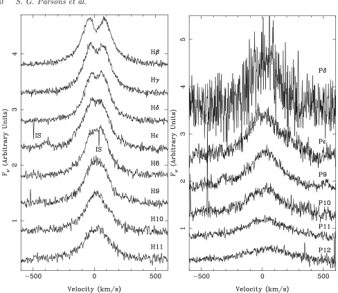
The most striking features of the UVES spectra are the emis-sion lines arising from the heated face of the secondary star, the most prominent of which are the Balmer lines. Figure 7
shows trailed spectra of several lines visible across the spec-tral range covered. The white dwarf component has been subtracted which creates a peak on the CaII trail that ap-pears to move in anti-phase with the secondary, due to in-terstellar absorption. The top row shows three Balmer lines (Hδ,Hγ and Hβ) which clearly show reversed cores, becom-ing more prominent at increasbecom-ing wavelength. Interestbecom-ingly, the same effect is not visible in the Paschen series. Large broadening is obvious in the Hydrogen lines.
[image:8.612.56.531.425.556.2]secondary star will be larger than that measured from these lines (see Section 4.4). The white dwarf component shown in Figure 6 was subtracted from each spectrum and the emis-sion lines fitted. Due to the presence of interstellar absorp-tion features, the subtracabsorp-tion of the white dwarf component creates peaks in the spectra since they show no phase vari-ation. Figure 8 shows the fit to several lines: all the Balmer lines fitted simultaneously (H11 to Hβ), several HeI lines fitted simultaneously and a fit to the MgII 4481˚A line. All the lines show a similar deviation from a sinusoidal shape at small and large phases (.0.25 and&0.75). This is because of the non-uniform distribution of flux over the secondary star. The radial velocity amplitude was calculated using only the points between these phases. The measured radial veloc-ity amplitude varies for each line, the Balmer lines showing a larger radial velocity amplitude than most of the other lines. In addition, the radial velocity amplitude of the Balmer lines decreases towards the higher energy states. We believe that the spread in measured values is related to the optical depth for each line; this is discussed in Section 4.4.
The Balmer, HeI and MgII lines from the UVES blue spectra were fitted with a polynomial and Gaussian. Fur-thermore, several HeI lines in the red spectra were fit as well as the Paschen lines (P12 to Pǫ). Although several FeI lines are seen, they are too faint to calculate the radial ve-locity amplitude of the secondary star reliably. Nonetheless, they do show the same phase dependant variations as all the other emission lines.
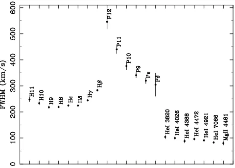
In addition to radial velocity information, the widths of the lines were fit. The widths of each of the emission lines vary strongly with phase and noticeable differences are seen between different atomic species. All of the hydrogen lines (both Balmer and Paschen lines) show a sharp increase in width around phase 0.1 which flattens off until phase 0.9 where the width falls off sharply. In contrast, the helium and magnesium lines show a gradual increase in width up to phase 0.5, then a gradual decrease. The behaviour of the hydrogen lines may be due to the lines saturating. Figure 9 shows the average width of a selection of lines around the secondary eclipse (phase 0.5). The most striking feature is the width of the hydrogen lines which are at least double the width of any other line and reach widths of almost 600 km s−1. An interesting trend is seen throughout the Balmer and Paschen series whereby the shorter wavelength lines are wider. The widths of these lines is probably an indication of Stark broadening which affects higher energy states to a larger extent. However, the longer wavelength Balmer lines become wider after Hδ (the slight increase in the width of the Hǫline is due to the overlapping CaII 3968˚A line and the nearby HeI 3965˚A line), presumably as a result of high optical depth leading to stronger saturation.
To recover the spectrum of the emitting region of the secondary star only, the simultaneous fit to all the HeI lines was used to shift the spectra to the frame of the emitting region of the secondary star. We use this radial velocity am-plitude since it lies in the centre of the measured amam-plitudes. The shifted spectra were then averaged, with larger weights given to those spectra taken around phase 0.5 where the reflection effect is greatest. Having previously subtracted the white dwarf’s spectrum, the result is the spectrum of only the irradiated part of the secondary star. The UVES blue arm spectrum of the secondary star is shown in
Fig-Figure 9.Widths of selected lines around the secondary eclipse, where they are at their widest. Note the large difference between the widths of the Hydrogen lines and that of every other species.
ure 10 with the identified lines labelled. As previously men-tioned, due to interstellar absorption lines, the subtraction of the white dwarf results in peaks that appear similar to the emission lines in Figure 10. These occur just before the HeI 4472˚A line and after the HeI 4713˚A line.
Once again the inverted core of the Balmer lines is the most striking feature. This can be seen even more clearly in Figure 11. For the shorter wavelength lines, there appears to be no core inversion. However, as the wave-length increases the effect becomes more pronounced. The separation between the two peaks in each line increases up to phase 0.5, reaching a maximum separation of 125 km s−1 for the Hβ line, the separation decreases symmet-rically around phase 0.5. This effect was found to be caused by departure from local thermodynamic equilibrium (LTE) (Barman et al. 2004). It is only seen in the hydrogen lines, and only the Balmer series. The Paschen lines, also shown in Figure 11, show no such core inversion.
The trailed spectra of the Balmer lines in Figure 7 show, in addition to the core inversion, a clear asymmetry be-tween the two peaks whereby the more shifted peak appears stronger (e.g. the most redshifted peak at phase 0.25 and the most blueshifted at phase 0.75). Barman et al. (2004) found that the line profiles of the hydrogen Balmer lines in non-LTE have reversed cores caused by an over-population of the
Precice mass and radius values for both components of the pre-CV NN Ser
9
Figure 10.Blue spectrum of the heated part of the secondary star. The white dwarf component has been subtracted. The peaks seen just before the HeI 4472˚A line and after the HeI 4713˚A line are a result of interstellar absorption lines being subtracted off and are not real emission lines.
optical depth of the line emission varies across the surface of the secondary star. The emission originating from the heavily irradiated region is optically thick (producing the double peaked profile explained by Barman et al. 2004). But further from this region, the irradiation flux decreases and the emission becomes more optically thin, changing the line profile towards a single peak. Since this region of optically thinner emission has a larger radial velocity amplitude, the
more shifted peak’s emission is increased resulting in the observed asymmetry.
Figure 11.Left: Profiles of the Balmer lines. IS corresponds to interstellar absorption features.Right: Profiles of the Paschen lines. The white dwarf component has been subtracted and the motion of the secondary star removed.
is visible. Hence it is necessary to allow for the variation in irradiation levels and hence the non-LTE core reversal in order to model the line profiles in NN Ser.
Non-LTE effects have also been seen in other pre-cataclysmic variable systems such as HS 1857+5144 (Aungwerojwit et al. 2007) where the Hβ and Hγ pro-files are clearly double-peaked, V664 Cas and EC 11575– 1845 (Exter et al. 2005) both show Stark broadened Balmer line profiles with absorption components. Likewise, double-peaked Balmer line profiles were observed in HS 1136+6646 (Sing et al. 2004) and Feige 24 (Vennes & Thorstensen 1994); GD 448 (Maxted et al. 1998) also shows an asym-metry between the two peaks of the core-inverted Balmer lines. Since NN Ser is the only system observed with echelle resolution it shows this effect more clearly than any other system.
The secondary star’s spectrum contains a large num-ber of emission lines throughout. Each line was identified using rest wavelengths obtained from the National
Insti-tute of Standards and Technology1 (NIST) atomic spectra database. The velocity offset (difference between the rest and measured wavelength) and FWHM of each line were obtained by fitting with a straight line and a Gaussian. The line flux and equivalent width (EW) were also measured. Table 4 contains a complete list of all the lines identified. In addition to the already known hydrogen, helium and cal-cium lines, there are a number of MgII lines throughout the spectra as well as FeI lines in the blue spectra and CI lines in the red spectra. The EW of the Balmer lines increases monotonically from H11 to Hβbut the core inversion causes the line flux to level off after the Hǫline. In addition to the Paschen P12 to Pδlines, half of the P13 line is seen (cut off by the spectral window used in the UVES upper red chip). The offsets for each line measured in Table 4 combined with the measured offset of the HeII absorption line from the white dwarf, give a measurement of the gravitational redshift of the white dwarf. The HeII absorption line has
Precice mass and radius values for both components of the pre-CV NN Ser
11
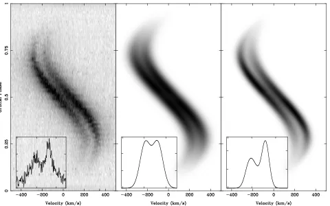
Figure 12.Left: trailed spectrum of the Hβline with the white dwarf and continuum subtracted.Centre: trailed spectrum of model line profiles convolved with two Gaussians set to reproduce the profile of the Hβ emission line.Right: trailed spectrum of a model with a varying line profile across the face of the secondary star, also set to reproduce the profile of the Hβemission line. Inset on each trail is the profile at phase 0.3; the first model fails to reproduce the observed asymmetry.
an offset of 25.6±2.7 km s−1 measured in the same way as for the emission lines. Taking a weighted average of the emission line velocities gives an offset of 15.1±0.2 km s−1, resulting in a gravitational redshift of 10.5±2.7 km s−1 for the white dwarf. This fairly small redshift is most likely due to the fact that the white dwarf is very hot leading to an inflated radius, as we will see shortly.
4 SYSTEM PARAMETERS 4.1 Light Curve Analysis
Analysis of the ULTRACAM light curves gives strong con-straints on the system parameters. A code written to pro-duce models for the general case of binaries containing a white dwarf was used (see Copperwheat et al. 2009, submit-ted, for details). It has been used in the study of other white dwarf-main sequence binaries (Pyrzas et al. 2009). Several components of the model include accretion phenomena for the analysis of cataclysmic variables. Since NN Ser is a de-tached system these components were not included. The pro-gram subdivides each star into small elements with a geom-etry fixed by its radius as measured along the direction of centres towards the other star. Roche geometry distortion and irradiation of the secondary star are included, the ir-radiation is approximated by σT′4
sec = σTsec4 +Firr where
T′
sec is the modified temperature andTsec the temperature of the unirradiated companion, σ is the Stefan-Boltzmann
constant andFirris the irradiating flux, accounting for the angle of incidence and distance from the white dwarf.
From an initial set of parameters defined by the user, the code produces model light curves which are initially fit-ted to the ULTRACAM data using Levenberg-Marquardt minimisation (Press et al. 1986) to produce a set of covari-ances. The resultant model parameters are fitted to the UL-TRACAM data using Markov chain Monte Carlo (MCMC) minimisation, using the covariances from the Levenberg-Marquardt minimisation to define the parameter jumps, to produce the final parameters and their errors; we follow the procedures described in Collier Cameron et al. (2007).
The parameters needed to define the model are: the mass ratio, q = Msec/MWD, the inclination, i, the radii scaled by the binary separation, RWD/a and Rsec/a, the unirradiated temperatures,Teff,WD and Teff,sec, linear limb darkening coefficients for the white dwarf and secondary star, the time of mid eclipse,T0, the period,P, the gravity darkening coefficient for the secondary star and the fraction of the irradiating flux from the white dwarf absorbed by the secondary star.
Table 4.Identified emission lines in the UVES spectra. Each line was fitted with a Gaussian to determine the velocity and FWHM.
Line ID Velocity FWHM Line Flux (10−15 Equivalent comment
(km s−1) (km s−1) ergs cm−2s−1˚A−1) Width (˚A)
H11 3770.634 16.4±1.5 250.7±4.1 3.10(4) 4.36(5) -H10 3797.910 12.6±1.1 233.9±2.9 3.46(4) 4.74(5) -HeI 3819.761 12.4±1.8 107.4±4.5 0.46(2) 0.69(3) -H9 3835.397 13.5±0.9 223.1±2.4 4.32(4) 6.30(6) -FeI 3856.327 11.0±3.7 63.2±9.9 0.12(1) 0.20(2) -FeI 3871.749 14.7±2.8 50.0±7.0 0.11(2) 0.20(3) -H8 3889.055 14.6±0.7 223.1±1.8 4.46(3) 6.51(4) -FeI 3906.479 10.1±3.6 68.2±8.8 0.22(2) 0.41(4)
-CaII 3933.663 -2.9±1.4 106.8±3.7 0.64(2) 1.06(3) Interstellar absorption present HeI 3964.727 12.2±3.2 85.7±8.0 0.30(2) 0.55(3) Close to the Hǫline
Hǫ3970.074 4.6±0.7 249.4±2.0 5.44(3) 9.59(6) -HeI 4026.189 14.3±1.0 96.3±2.8 0.71(2) 1.28(3) -Hδ4101.735 17.1±0.6 231.0±1.5 4.72(3) 8.57(5) -HeI 4120.824 10.3±4.4 73.9±9.8 0.12(1) 0.24(2) -HeI 4143.759 15.6±2.5 85.2±6.4 0.29(1) 0.59(3) -FeI 4266.964 12.8±4.5 97.9±10.5 0.22(2) 0.49(3) -Hγ4340.465 14.5±0.6 255.9±1.5 4.74(2) 9.40(4) -HeI 4387.928 18.1±1.4 80.7±3.6 0.34(1) 0.74(2) -FeI 4415.122 15.5±4.4 66.4±11.1 0.18(1) 0.42(2) -HeI 4471.681 14.5±1.0 86.3±2.5 0.54(2) 1.15(2) -MgII 4481.327 16.9±1.3 89.5±3.5 0.33(1) 0.74(2) -FeI 4649.820 18.9±4.6 80.7±8.8 0.13(1) 0.30(2) -HeI 4713.146 14.7±1.4 76.6±3.7 0.12(1) 0.57(2) -Hβ4861.327 14.7±0.4 262.0±1.3 4.26(2) 10.34(4) -HeI 4921.929 16.4±1.0 81.7±2.5 0.39(1) 1.05(2) -HeI 7065.709 15.4±0.4 78.4±1.1 0.27(3) 1.17(1) -HeI 7281.349 16.0±0.7 67.3±2.0 0.13(3) 0.64(1) -MgII 7877.051 12.6±3.1 37.1±7.8 0.12(3) 0.23(2) -MgII 7896.368 12.9±2.2 54.8±5.7 0.15(4) 0.30(2) -CI 8335.15 9.9±4.1 44.2±6.6 0.11(4) 0.20(3) -CaII 8498.02 14.4±2.7 99.8±8.3 0.14(5) 0.90(3)
-P12 8750.473 16.6±5.3 402.4±16.8 1.15(2) 5.49(1) Half of P13 line seen as well P11 8862.784 16.5±2.7 376.2±8.0 1.68(2) 8.16(9)
-CaII 8927.36 18.0±3.6 58.3±9.5 0.13(1) 0.65(5) -P10 9014.911 13.1±2.7 280.4±8.1 1.97(2) 10.27(9) -CI 9061.43 12.1±4.6 35.6±7.7 0.12(3) 0.28(4)
-MgII 9218.248 16.2±2.6 48.9±7.6 0.12(6) 0.51(4) Close to the P9 line P9 9229.015 15.1±1.3 316.5±3.6 2.42(2) 11.47(8)
-MgII 9244.266 16.0±2.5 44.6±6.4 0.14(3) 0.40(3) -CI 9405.73 10.7±5.1 46.0±8.0 0.15(1) 0.87(7) -Pǫ9545.972 16.4±2.3 332.3±6.4 3.39(4) 19.58(7)
-Pδ10049.374 18.4±7.4 253.4±22.2 2.7(1) 18.0(7) Very noisy in the far red
dwarf withTeff = 57,000K and logg= 7.46 using ULTRA-CAMu’g’r’i’z’ filters (G¨ansicke et al. 1995). The loggwas obtained from an initial MCMC minimisation of theg’ light curve with the limb darkening coefficient of the white dwarf fixed at a value of 0.2 (the logg determined from this is very similar to the final value determined later). All other parameters were optimised in the MCMC minimisation. The initial values for the inclination, radii and the temperature of the secondary star were taken from Haefner et al. (2004), the limb darkening coefficient for the secondary star was ini-tially set to zero and the fraction of the irradiating flux from the white dwarf absorbed by the secondary star was initially set to 0.5 (note that the intrinsic flux of the secondary star is negligible).
Since phase-binned light curves were used,T0was set to zero but allowed to change while the period was kept fixed at
Precice mass and radius values for both components of the pre-CV NN Ser
13
Table 5.Best fit parameters from Markov chain Monte Carlo minimisation for each ULTRACAM light curve. Lin limb is the linear limb darkening coefficient for the white dwarf which was kept fixed, the values quoted are for a model white dwarf of temperature 57,000K and logg= 7.46. Absorb is the fraction of the irradiating flux from the white dwarf absorbed by the secondary star.
Parameter u’ g’ r’ i’
Inclination 89.18±0.27 89.67±0.05 89.31±0.21 89.59±0.27
RWD/a 0.02262±0.00014 0.02264±0.00002 0.02271±0.00010 0.02257±0.00010 Rsec/a 0.1660±0.0011 0.1652±0.0001 0.1657±0.0007 0.1654±0.0003 Tsec 3962±32 3125±10 3108±11 3269±7
Lin limbWD 0.125 0.096 0.074 0.060
Lin limbsec −1.44±0.13 −0.48±0.03 −0.26±0.02 −0.06±0.03
Absorb 0.899±0.001 0.472±0.001 0.604±0.006 0.651±0.005
curves and 2.1 for the u’ light curve. The MCMC chains showed no variation beyond that expected from statistical variance and the probability distributions are symmetrical and roughly Gaussian.
The errors in Table 5 were scaled to give a reduced
χ2= 1. The inclination was determined by taking a weighted average and is found to be 89.6◦±0.2◦. This inclination is
much higher than the 84.6◦ determined by Haefner et al.
(2004) but is consistent with the inferred inclination of
∼88◦ from Brinkworth et al. (2006). The scaled radius of
the white dwarf isRWD/a= 0.0226±0.0001 and the scaled radius of the secondary star isRsec/a= 0.165±0.001. Given our black body assumption,Tsecdoes not represent the true temperature of the secondary star, it is effectively just a scal-ing factor. An interestscal-ing trend is seen in the limb darken-ing coefficients for the secondary star, which are all negative (limb brightening), the amount of limb brightening decreases with increasing wavelength. This is presumably the result of seeing to different depths at different wavelengths.
Although the ULTRACAMz’ photometry was of fairly poor quality (owing to conditions), it was good enough to measure the magnitude of the secondary star during the primary eclipse. A zeroth-order polynomial was fit to ther’,
i’ andz’ filter light curves during the primary eclipse. The measured magnitudes were:r’= 21.8±0.1,i’= 20.4±0.1 and
z’= 19.6±0.1, which gives colours of (r’-i’)sec= 1.4±0.1 and (i’-z’)sec = 0.8±0.1 which corresponds to a spectral type of M4±0.5 (West et al. 2005). This is consistent with the results of Haefner et al. (2004) who fitted the spectral fea-tures of the secondary star taken during the primary eclipse to determine a spectral type of M4.75±0.25.
4.2 Heating of the Secondary Star
One can make an estimate of the heating effect by compar-ing the intrinsic luminosity of the secondary star to that ceived from the white dwarf. We use the mass-luminosity re-lation from Scalo et al. (2007) determined by fitting a poly-nomial to the luminosities and binary star masses compiled by Hillenbrand & White (2004) to determine the luminosity of the secondary star as 1.4×10⁻³L
⊙. The luminosity of the
white dwarf was calculated usingLWD = 4πR2σT4. Using the radius derived in Section 4.4 and the temperature from Haefner et al. (2004) gives the luminosity of the white dwarf as 4.2 L⊙. Using the scaled radius of the secondary star from
Table 5 translates to the secondary star being hit by over 20 times its own luminosity. Despite this, the colours (hence spectral type) of the unirradiated side are in agreement with the derived mass (Baraffe & Chabrier 1996) (see Section 4.4 for the mass derivation) showing that this extreme heating effect on one hemisphere of the secondary star has no mea-surable effect on the unirradiated hemisphere.
4.3 Distance to NN Ser
Absolute magnitudes for the white dwarf in NN Ser were calculated using a model from Holberg & Bergeron (2006) for a DA white dwarf of mass 0.527M⊙, logg = 7.5 and
a temperature of 60,000K which most closely matched the parameters found for NN Ser. We give an uncertainty of
[image:15.612.305.556.154.237.2]±0.1 magnitudes for the absolute magnitudes based on the
Table 6.Distance measurements from each of the ULTRACAM light curves. The absolute magnitudes for the white dwarf in NN Ser were obtained from Holberg & Bergeron (2006) with an error of±0.1 magnitudes.
Filter Absolute Measured Extinction Distance Magnitude Magnitude (mags) (pc)
u’ 7.264 15.992±0.006 0.258±0.258 494±63
g’ 7.740 16.427±0.002 0.190±0.190 501±49
r’ 8.279 16.931±0.004 0.138±0.138 505±40
i’ 8.666 17.309±0.004 0.104±0.104 510±34
z’ 9.025 17.71±0.01 0.074±0.074 527±30
uncertainty in temperature from Haefner et al. (2004) and its effect on the models of Holberg & Bergeron (2006). The magnitudes of the white dwarf in NN Ser were calculated by fitting a zeroth-order polynomial to the flat regions either side of the primary eclipse with a correction made for the flux of the secondary star. Using the reddening value of E(B-V)= 0.05±0.05 from Wood & Marsh (1991) we correct the apparent magnitudes using the conversion of Schlegel et al. (1998). From these a distance was calculated for each of the ULTRACAM filters. Table 6 lists the distances calcu-lated in each of these filters. Using these values gives a dis-tance to NN Ser of 512±43 pc consistent with the result of Haefner et al. (2004) of 500±35 pc.
The galactic latitude of NN Ser is 45.3◦ which,
com-bined with the derived distance, gives NN Ser a galactic scale height of 364±31 pc. The proper motion of NN Ser was retrieved from the US Naval Observatory (USNO) Im-age and Catalogue Archive. The archive values areµRA =
−0.020±0.003 andµDEC=−0.056±0.004 arcsec / yr. At the derived distance this corresponds to a transverse velocity for NN Ser of 160±14 km s−1.
4.4 Ksec correction
The emission lines seen in the UVES spectra are the re-sult of reprocessed light from the surface of the secondary star facing the white dwarf. Hence, their radial velocity am-plitude represents a lower limit to the true centre of mass radial velocity amplitude. For accurate mass determinations the centre of mass radial velocity amplitude is required thus we need to determine the deviation between the reprocessed light centre and the centre of mass for the secondary star. We do this by computing model line profiles from the irra-diated face.
Precice mass and radius values for both components of the pre-CV NN Ser
15
Figure 14. Light curves of various lines over-plotted with an optically thick (narrower) and thin (wider) model with the same measuredKsecas the line. The model light curves are scaled to
match the flux level of the lines around phase 0.5. The Hβline is optically thick, the MgII line is optically thin and the HeI line is somewhere between thick and thin.
an indication of the instrumental resolution, which we found to be 5 km s−1(FWHM) for the UVES blue chip.
As mentioned previously, the measured radial velocity amplitude varies for each line. We believe that this scatter is the result of differences in optical depths of the lines, which will affect the angular distribution of line flux from any given point on the star resulting in a range of observed radial velocity amplitudes. Hence, the model is required to produce line profiles over a continuous range of optical depths (see Appendix for details of the model).
[image:16.612.43.284.88.530.2]The radiation from the secondary star is modelled as a slab of constant optical depth (τ0) and the source func-tion changes exponentially with depth, the factor that deter-mines how this changes isβ(i.e. the source function changes
Table 7.Measured and corrected values of Ksec with the best
fit model line profiles parameters, for several lines in the UVES blue spectra.
Line τ0 β Ksec,meas Ksec,corr q
km s−1 km s−1
HeI 3820 2 −0.75 252.2±1.9 296.7±1.9 0.210(6) HeI 4026 1 −3 257.7±1.7 300.1±1.7 0.208(6) HeI 4388 1 −10 249.9±2.0 300.2±2.0 0.208(6) HeI 4472 1 −1.5 263.1±1.8 305.2±1.8 0.204(6) HeI 4922 1 −0.5 255.6±1.8 296.9±1.8 0.210(6) Hβ 100 −1.5 271.1±1.9 307.6±1.9 0.203(6) Hγ 100 −1.5 265.1±1.9 302.9±1.9 0.206(6) Hδ 50 −1.5 265.0±1.9 298.1±1.9 0.209(6) Hǫ 5 −1.25 263.2±1.9 304.4±1.9 0.205(6) H8 5 −1 262.5±1.9 303.2±1.9 0.206(6) H9 2 −0.5 258.1±1.9 297.4±1.9 0.210(6) H10 2 −0.75 257.2±2.1 299.9±2.1 0.208(6) H11 1 −2 259.3±2.1 301.2±2.1 0.207(6) MgII 4481 0.005 −1.25 252.8±1.8 298.7±1.8 0.209(6)
with vertical optical depth (τ) as eβτ), this allows one to
have a continuous transition from optically thin to thick and to have limb darkening or brightening. We keepKWDfixed at the measured value of 62.3 km s−1, and just changeK
sec. We measured the radial velocity amplitude of the resulting line profiles in the same way as for the emission lines in the UVES spectra. Initially,Ksecwas set to give a measured ra-dial velocity amplitude of 252.8 km s−1(the measured radial velocity amplitude of the MgII 4482˚A line) and the values of the total vertical optical depth and source function ex-ponential factor were allowed to vary. The light curves pro-duced were fitted to the MgII 4481˚A line light curve using least squares fitting to determine the optimal values forτ0 andβ. This was repeated for several lines in the UVES blue spectra adjustingKsecto produce the measured radial veloc-ity amplitude for that line. Figure 14 shows the light curve for three different lines over plotted with an optically thick and optically thin model. For the Hβ line, the emission is optically thick, the MgII line is optically thin and the HeI line lies somewhere between these two extremes (the white dwarf component was subtracted from all the light curves). Table 7 lists the best fit values forτ0andβfor each line and the measured and correctedKsecandqvalues.
[image:16.612.304.556.142.316.2]The MgII 4481˚A line appears to be the closest to the optically thin model. As such it probably provides the most accurate correction since, in the optically thin case, the an-gular distribution of the line flux from any given point on the star is even, removing any dependence upon this. Even so, all the corrected values are consistent to within a few km s−1. The first few Balmer lines (Hβto Hδ) are optically thick but as the series progresses, the lines become more optically thin. There also appears to be a small increase in the value ofβ throughout the series (with the exception of H10 and H11). The helium lines appear to be somewhere between optically thick and thin.
Figure 15.Bottom: MeasuredKsecfor several lines in the UVES
blue spectra from Gaussian fitting and their corrected values (top). The CaII line is contaminated by interstellar absorption which was fitted as an additional Gaussian component and was not corrected. The fit to all the Balmer lines simultaneously is the point labelled ‘balmers’. The point labelled ‘HeI’s’ is a fit to all the visible HeI lines whilst the point labelled ‘single HeI’s’ is a fit to only the HeI lines which have a single component (i.e. the intensity is not shared by several lines).
error in the correction is dominated by systematic effects from the model and fitting process, for which we estimate an error of 3 km s−1 for the radial velocity amplitude of the secondary star. Some simple considerations can give an idea of the largest possible error we might have made in cor-recting theK values. The distance from the centre of the mass to the sub-stellar point in terms of velocity is given by (KWD+Ksec)Rsec/a= 60 km s−1; this is maximum possi-ble correction. A lower limit comes from assuming the emis-sion to be uniform over the irradiated face of the secondary. Then the centre of light is 0.42 of the way from the cen-tre of mass to the sub-stellar point (Wade & Horne 1988), leading to a lower limit on the correction of 24 km s−1. The corrections from our model range from 33 to 46 km s−1, in the middle of these extremes.
From the corrected value andKWD= 62.3±1.9 km s−1 we determine the mass ratio asq =Msec/MWD = 0.207± 0.006. Using this, the mass of the white dwarf is then deter-mined using Kepler’s third law
P K3 sec 2πG =
MWDsin3i
(1 +q)2 , (4)
using the period (P) from Brinkworth et al. (2006). This gives a value ofMWD= 0.535±0.012 M⊙. The mass ratio
then gives the mass of the secondary star asMsec= 0.111± 0.004 M⊙. Knowing the masses, the orbital separation is
found using
a3=G(MWD+Msec)P 2
4π2 , (5)
which gives a value of a = 0.934±0.009 R⊙. Using this
gives the radii of the two stars as RWD = 0.0211±0.0002 R⊙ and Rsec = 0.154±0.002 R⊙. The radius of the
sec-ondary star in our model is measured from the centre of
Table 8.System parameters. (1) this paper; (2) Brinkworth et al. (2006); (3) Haefner et al. (2004). WD: white dwarf, Sec: sec-ondary star.
Parameter Value Ref.
Period (days) 0.13008017141(17) (2)
Inclination 89.6±0.2◦ (1)
Binary separation 0.934±0.009 R⊙ (1)
Mass ratio 0.207±0.006 (1)
WD mass 0.535±0.012 M⊙ (1)
Sec mass 0.111±0.004 M⊙ (1)
WD radius 0.0211±0.0002 R⊙ (1)
Sec radius polar 0.147±0.002 R⊙ (1)
Sec radius sub-stellar 0.154±0.002 R⊙ (1)
Sec radius backside 0.153±0.002 R⊙ (1)
Sec radius side 0.149±0.002 R⊙ (1)
Sec radius volume-averaged 0.149±0.002 R⊙ (1)
WD logg 7.47±0.01 (1)
WD temperature 57000±3000 K (3)
KWD 62.3±1.9 km s−1 (1)
Ksec 301±3 km s−1 (1)
WD grav. redshift 10.5±2.7 km s−1 (1)
WD type DAO1 (3)
Sec spectral type M4±0.5 (1)
Distance 512±43 pc (1)
WD hydrogen layer fractional mass 10−4 (1)
mass towards the white dwarf and hence is larger than the average radius of the secondary star. The radius as mea-sured towards the backside is Rsec,back = 0.153 R⊙, the
polar radius is Rsec,pol = 0.147 R⊙ and perpendicular to
theseRsec,side= 0.149 R⊙. The volume-averaged radius is Rsec,av= 0.149±0.002 R⊙.
The surface gravity of the white dwarf is given by
g=GMWD
RWD2
, (6)
which gives a value of logg= 7.47±0.01.
5 DISCUSSION
[image:17.612.305.552.143.378.2]consis-Precice mass and radius values for both components of the pre-CV NN Ser
17
Figure 16. Mass-radius plot for white dwarfs measured inde-pendent of any mass-radius relations. Data from Provencal et al. (1998), Provencal et al. (2002) and Casewell et al. (2009) are plotted. The filled circles are visual binaries and the open cir-cles are common proper-motion systems. The solid lines corre-spond to different carbon-oxygen core pure hydrogen atmosphere models. The first number is the temperature, in thousands of degrees, the second number is the hydrogen layer thickness (i.e. lines labelled -4 have a thickness of MH/MWD = 10−4) from
Holberg & Bergeron (2006) and Benvenuto & Althaus (1999). The dashed line is the zero-temperature mass-radius relation of Eggleton from Verbunt & Rappaport (1988).
tent with the inflated radius of the white dwarf due to its high temperature.
Since visual binary systems and common proper-motion systems still rely on model atmosphere calculations to de-termine radii, the white dwarf in NN Ser is one of the first to have its mass and radius measured independently. O’Brien et al. (2001) determine the mass and radius of both components of the eclipsing PCEB V471 Tau independently however, since they did not detect a secondary eclipse, they had to rely on less direct methods to determine the radius of the secondary and the inclination. This demonstrates the value of eclipsing PCEBs for investigating the mass-radius relation for white dwarfs.
In addition, the mass and radius of the secondary star have been determined independently of any mass-radius re-lation. Since this is a low mass star it helps improve the statistics for these objects and our values are more precise than the majority of comparable measurements. Figure 17 shows the position of the secondary star in NN Ser (using the volume-averaged radius) in relation to other low mass stars with masses and radii determined independently of any mass-radius relation (although the masses of the single stars were determined using mass-luminosity relations). For very low mass stars (M . 0.3 M⊙) the current errors on mass
and radius measurements are so large that that one can ar-gue the data are consistent with the low-mass models. How-ever, the secondary star in NN Ser appears to be the first object with errors small enough to show an inconsistency with the models. The measured radius is 10% larger than predicted by the model. However, irradiation increases the radius of the secondary star. For the measured radius of the secondary star in NN Ser, the work of Ritter et al. (2000)
Figure 17. Mass-radius plot for low mass stars. Data from L´opez-Morales (2007) and Beatty et al. (2007). The filled circles are secondaries in binaries, the open circles are low mass bina-ries and the crosses are single stars. The solid line represents the theoretical isochrone model from Baraffe et al. (1998), for an age of 0.4 Gyr, solar metalicity, and mixing lengthα= 1.0, the dot-ted line is the same but for an age of 4 Gyr. The position of the secondary star in NN Ser is also shown if there were no irradia-tion effects. The masses of the single stars were determined using mass-luminosity relations.
and Hameury & Ritter (1997) gives an inflation of 5.6%. The un-irradiated radius is also shown in Figure 17 and is consis-tent with the models. Hence the secondary star in NN Ser supports the theoretical mass-radius relation for very low mass stars. Potentially, an initial-final mass relation could be used to estimate the age of NN Ser, but since the system has passed through a common envelope phase its evolution may have been accelerated and the white dwarf may be less massive than a single white dwarf with the same progenitor mass leading to an overestimated age. In addition, the mass of the white dwarf in NN Ser is close to the mean white dwarf mass and the initial-final mass relation is flat in this region. This means a large range of progenitor masses are possible for the white dwarf and hence a large range in age, this means a reliable estimate of the age of NN Ser is not possible. In any case, the position of the un-irradiated sec-ondary star is also consistent with a similarly large range of ages. The mass and radius of the secondary star support the argument of Brinkworth et al. (2006) that it is not ca-pable of generating enough energy to drive period change via Applegate’s mechanism (Applegate 1992).
The system parameters determined for NN Ser are sum-marised in Table 8. Using the UVES spectra, the gravita-tional redshift of the white dwarf was found to be 10.5±2.7 km s−1. Using the measured mass and radius from Table 8 gives a redshift of 16.1 km s−1, correcting for the redshift of the secondary star (0.5 km s−1), the difference in trans-verse Doppler shifts (0.15 km s−1) and the potential at the secondary star owing to the white dwarf (0.3 km s−1) gives a value of 15.2±0.5 km s−1 which is consistent with the measured value to∼2 sigma, although in this case, the
[image:18.612.45.283.95.278.2]6 CONCLUSIONS
We have measured precise masses and radii of the white dwarf and M dwarf components of the post common en-velope binary NN Serpentis using UVES spectroscopy and ULTRACAM photometry.
Using the HeII 4686˚A absorption line from the white dwarf we determined the radial velocity amplitude of the white dwarf directly from the spectra. Using a number of emission lines in the UVES spectra originating from the heated face of the secondary star, we were able to correct the radial velocity amplitude of the secondary star from the heated face to the centre of mass of the secondary star itself. From analysis of ULTRACAM light curves we deter-mine a system inclination of 89.6◦±0.2◦, higher than the
value of 84.6◦±1.1◦found by Haefner et al. (2004) which,
along with our direct determination ofKWD, leads to a lower mass ratio than previously derived. The radius of the white dwarf is found to beRWD= 0.0211±0.0002 R⊙, larger than
in previous studies but, given its temperature, is consistent with its derived mass of MWD = 0.535±0.012 M⊙. The
mass and radius of the white dwarf show excellent agree-ment with a hot carbon-oxygen core white dwarf with a ‘thick’ hydrogen layer of fractional mass MH/MWD= 10−4. The mass of the secondary star is found to beMsec = 0.111±0.004 M⊙ with a volume-averaged radius ofRsec= 0.149±0.002 R⊙, which is smaller than previously
deter-mined. The radius of the secondary star is consistent with models if a ∼6% correction is made for the irradiation it receives from the white dwarf.
The ULTRACAM photometry also provided colours for the secondary star and thus a spectral type. This was con-sistent with the derived mass showing that, despite being irradiated by over 20 times its own luminosity, there is very little backside heating, although infrared data are needed to determine this more accurately. Finally, using model white dwarf data we determine a distance to NN Ser of 512±43 pc, consistent with previous studies.
ACKNOWLEDGEMENTS
We thank the referee, M Burleigh, for his useful comments and suggestions. TRM, CMC and BTG acknowledge sup-port from the Science and Technology Facilities Council (STFC) grant number ST/F002599/1. SPL acknowledges the support of an RCUK Fellowship. ULTRACAM, VSD and SPL are supported by STFC grants ST/G003092/1 and PP/E001777/1. The results presented in this paper are based on observations collected at the European Southern Observatory (La Silla) under programme ID 073.D-0633 and with the William Herschel Telescope operated on the island of La Palma by the Isaac Newton Group in the Spanish Observatorio del Roque de los Muchachos of the Institu-tions de Astrofisica de Canarias. We used SIMBAD, main-tained by the Centre de Donn´ees astronomiques de Stras-bourg, and the National Aeronautics and Space Adminis-tration (NASA) Astrophysics Data System. This research has made use of the USNOFS Image and Catalogue Archive operated by the United States Naval Observatory, Flagstaff Station and the National Institute of Standards and Tech-nology (NIST) Atomic Spectra Database (version 3.1.5).
STScI is operated by the Association of Universities for Re-search in Astronomy inc.
REFERENCES
Applegate J. H., 1992, ApJ, 385, 621
Aungwerojwit A., G¨ansicke B. T., Rodr´ıguez-Gil P., Hagen H.-J., Giannakis O., Papadimitriou C., Allende Prieto C., Engels D., 2007, A&A, 469, 297
Baraffe I., Chabrier G., 1996, ApJ, 461, L51+
Baraffe I., Chabrier G., Allard F., Hauschildt P. H., 1998, A&A, 337, 403
Barman T. S., Hauschildt P. H., Allard F., 2004, ApJ, 614, 338
Beatty T. G., Fern´andez J. M., Latham D. W., Bakos G. ´A., Kov´acs G., Noyes R. W., Stefanik R. P., Torres G., Everett M. E., Hergenrother C. W., 2007, ApJ, 663, 573
Benvenuto O. G., Althaus L. G., 1999, MNRAS, 303, 30 Brinkworth C. S., Marsh T. R., Dhillon V. S., Knigge C.,
2006, MNRAS, 365, 287
Casewell S. L., Dobbie P. D., Napiwotzki R., Burleigh M. R., Barstow M. A., Jameson R. F., 2009, MNRAS, 395, 1795
Catalan M. S., Davey S. C., Sarna M. J., Connon-Smith R., Wood J. H., 1994, MNRAS, 269, 879
Collier Cameron A. et al., 2007, MNRAS, 380, 1230 Copperwheat C. M., Marsh T. M., Dhillon V. S., Littlefair
S. P., Hickman R., G¨ansicke B. T., Southworth J., 2009, MNRAS, 0, 0
Dekker H., D’Odorico S., Kaufer A., Delabre B., Kot-zlowski H., 2000, in Iye M., Moorwood A. F., eds, So-ciety of Photo-Optical Instrumentation Engineers (SPIE) Conference Series Vol. 4008 of Presented at the Society of Photo-Optical Instrumentation Engineers (SPIE) Con-ference, Design, construction, and performance of UVES, the echelle spectrograph for the UT2 Kueyen Telescope at the ESO Paranal Observatory. pp 534–545
Dhillon V. S., Marsh T. R., Stevenson M. J., Atkinson D. C., Kerry P., Peacocke P. T., Vick A. J. A., Beard S. M., Ives D. J., Lunney D. W., McLay S. A., Tierney C. J., Kelly J., Littlefair S. P., Nicholson R., Pashley R., Harlaftis E. T., O’Brien K., 2007, MNRAS, 378, 825 Exter K. M., Pollacco D. L., Maxted P. F. L., Napiwotzki
R., Bell S. A., 2005, MNRAS, 359, 315
G¨ansicke B. T., Beuermann K., de Martino D., 1995, A&A, 303, 127
Green R. F., Ferguson D. H., Liebert J., Schmidt M., 1982, PASP, 94, 560
Haefner R., 1989, A&A, 213, L15
Haefner R., Fiedler A., Butler K., Barwig H., 2004, A&A, 428, 181
Hameury J.-M., Ritter H., 1997, A&AS, 123, 273 Hillenbrand L. A., White R. J., 2004, ApJ, 604, 741 Holberg J. B., Bergeron P., 2006, AJ, 132, 1221 Hubeny I., 1988, Comput.,Phys.,Comm., 52, 103 Hubeny I., Lanz T., 1995, ApJ, 439, 875
Littlefair S. P., Dhillon V. S., Marsh T. R., G¨ansicke B. T., Southworth J., Baraffe I., Watson C. A., Copperwheat C., 2008, MNRAS, 388, 1582
Precice mass and radius values for both components of the pre-CV NN Ser
19
Maxted P. F. L., Marsh T. R., Moran C., Dhillon V. S., Hilditch R. W., 1998, MNRAS, 300, 1225
O’Brien M. S., Bond H. E., Sion E. M., 2001, ApJ, 563, 971
Press W. H., Flannery B. P., Teukolsky S. A., 1986, Numer-ical recipes. The art of scientific computing. Cambridge: University Press, 1986
Provencal J. L., Shipman H. L., Hog E., Thejll P., 1998, ApJ, 494, 759
Provencal J. L., Shipman H. L., Koester D., Wesemael F., Bergeron P., 2002, ApJ, 568, 324
Pyrzas S., G¨ansicke B. T., Marsh T. R., Aungwerojwit A., Rebassa-Mansergas A., Rodr´ıguez-Gil P., Southworth J., Schreiber M. R., Nebot Gomez-Moran A., Koester D., 2009, MNRAS, 394, 978
Renzini A., Bragaglia A., Ferraro F. R., Gilmozzi R., Or-tolani S., Holberg J. B., Liebert J., Wesemael F., Bohlin R. C., 1996, ApJ, 465, L23+
Ritter H., Zhang Z.-Y., Kolb U., 2000, A&A, 360, 969 Scalo J., Kaltenegger L., Segura A. G., Fridlund M., Ribas
I., Kulikov Y. N., Grenfell J. L., Rauer H., Odert P., Leitzinger M., Selsis F., Khodachenko M. L., Eiroa C., Kasting J., Lammer H., 2007, Astrobiology, 7, 85 Schlegel D. J., Finkbeiner D. P., Davis M., 1998, ApJ, 500,
525
Schmidt H., 1996, A&A, 311, 852
Schreiber M. R., G¨ansicke B. T., 2003, A&A, 406, 305 Sing D. K., Holberg J. B., Burleigh M. R., Good S. A.,
Barstow M. A., Oswalt T. D., Howell S. B., Brinkworth C. S., Rudkin M., Johnston K., Rafferty S., 2004, AJ, 127, 2936
Sion E. M., Greenstein J. L., Landstreet J. D., Liebert J., Shipman H. L., Wegner G. A., 1983, ApJ, 269, 253 Smith J. A. et al., 2002, AJ, 123, 2121
Vennes S., Thorstensen J. R., 1994, AJ, 108, 1881 Verbunt F., Rappaport S., 1988, ApJ, 332, 193 Wade R. A., Horne K., 1988, ApJ, 324, 411
West A. A., Walkowicz L. M., Hawley S. L., 2005, PASP, 117, 706
Wood J. H., Marsh T. R., 1991, ApJ, 381, 551 Wood M. A., 1992, ApJ, 386, 539
APPENDIX A: MODELLING OF THE IRRADIATION LINES
The radial velocity semi-amplitudes we measure for the emission lines in NN Ser reflect the distance from the cen-tre of mass of the binary of the irradiated face of the sec-ondary star. To obtain the semi-amplitude of the secsec-ondary star,Ksec, we need to correct for the distance from the flux-weighted mean of the irradiated flux to the centre of mass of the secondary. To do this we need to know the size of the secondary star, which we know accurately from photometry, but also the distribution of flux. We adopted an empirical modelling approach which is described in this section.
To model the irradiated flux we modelled the surface of the secondary star as a series of small elements, allowing for the (small) distortion from tidal and centrifugal forces. The intensity of irradiated flux from each point was set to be lin-early proportional to the incident flux from the white dwarf allowing for inverse square law dilution and incident angle.
Our ultimate goal was to simulate the line profiles so that we could measure radial-velocities from them to allow us to adjustKsec until we matched the observed semi-amplitude. As Table 7 and Figure 15 show however, the observed semi-amplitudes varied from line to line over a range of 20 km s−1. We believe that this reflects differences in optical depths in the lines, which will affect the angular distribution of line flux from any given point on the star. For instance, if the flux is preferentially beamed perpendicular to the stellar surface, then at the quadrature phases, we will see the limb of the irradiated region more prominently compared to the region of maximum irradiation than we would otherwise. This will lead to a higher observed semi-amplitude. To allow for such effects we devised a simple model of the line emitting region, which we now describe.
A1 Optical depth model
We wanted to be able to model optically thin and optically thick emitting regions within one model so that there was a continuous transition from one to the other. To do so we assumed a simple model in which the line emitting region at any point on the secondary behaves as if it had a total vertical optical depthτ0, and a source function given by an exponential function of vertical optical depth,τ,
S(τ)∝eβτ,
whereβis a user-defined constant allowing the source func-tion to increase or decrease with optical depth. To prevent divergent integrals, we must have thatβ < 1. For β > 0, the source function increases as one goes further into the star and we expect limb darkening, whileβ <0 gives limb brightening. Asτ0→0, we obtain optically-thin behaviour, thus this two-parameter model gives the desired modelling freedom.
For an incident angleθ such thatµ= cosθ, the emer-gent intensity is then given by
I(µ)∝ Z τ0
0
eβτe−τ /µdτ µ,
where the variable of integration τ is the vertical optical depth while the optical depth along the line of sight isτ /µ. Therefore
I(µ)∝1−exp(β−1/µ)τ0
1−βµ .
In the limitτ0→ ∞we have
I(µ)∝ 1
1−βµ,
which for smallβgivesI(µ)∝1+βµ, giving limb-darkening or brightening as expected. In the optically thin limit,τ0→ 0,
I(µ)∝τ0 µ.
is why lines such as MgII which have light-curves close to the optically-thin case have the lowest semi-amplitudes.
A2 Selecting τ0 and β