White Rose Research Online
Universities of Leeds, Sheffield and York
http://eprints.whiterose.ac.uk/
This is a copy of the final published version of a paper published via gold open access
in
PLoS ONE
.
This open access article is distributed under the terms of the Creative Commons
Attribution Licence (
http://creativecommons.org/licenses/by/3.0
), which permits
unrestricted use, distribution, and reproduction in any medium, provided the
original work is properly cited.
White Rose Research Online URL for this paper:
http://eprints.whiterose.ac.uk/83974
Published paper
Fish, K.E., Collins, R., Green, N.H., Sharpe, R.L., Douterelo, I., Osborn, A.M. and
Boxall, J.B. (2015) Characterisation of the Physical Composition and Microbial
Community Structure of Biofilms within a Model Full-Scale Drinking Water
Distribution System. PLoS ONE, 10 (2). e0115824 . Doi:
Characterisation of the Physical Composition
and Microbial Community Structure of
Biofilms within a Model Full-Scale Drinking
Water Distribution System
Katherine E. Fish1,2*, Richard Collins1, Nicola H. Green3, Rebecca L. Sharpe4, Isabel Douterelo1, A. Mark Osborn5, Joby B. Boxall1
1Pennine Water Group, Department of Civil and Structural Engineering, The University of Sheffield, Sheffield, United Kingdom,2NERC Biomolecular Analysis Facility, Department of Animal and Plant Sciences, Western Bank, Sheffield, United Kingdom,3Kroto Research Institute, The University of Sheffield, Sheffield, United Kingdom,4Department of the Natural & Built Environment, Sheffield Hallam University, Sheffield, United Kingdom,5School of Applied Sciences, RMIT University, PO Box 71 Bundoora, Melbourne, Australia
Abstract
Within drinking water distribution systems (DWDS), microorganisms form multi-species biofilms on internal pipe surfaces. A matrix of extracellular polymeric substances (EPS) is produced by the attached community and provides structure and stability for the biofilm. If the EPS adhesive strength deteriorates or is overcome by external shear forces, biofilm is mobilised into the water potentially leading to degradation of water quality. However, little is known about the EPS within DWDS biofilms or how this is influenced by community composition or environmental parame-ters, because of the complications in obtaining biofilm samples and the difficulties in analysing EPS. Additionally, although biofilms may contain various microbial groups, research commonly focuses solely upon bacteria. This research applies an EPS analysis method based upon fluo-rescent confocal laser scanning microscopy (CLSM) in combination with digital image analysis (DIA), to concurrently characterize cells and EPS (carbohydrates and proteins) within drinking water biofilms from a full-scale DWDS experimental pipe loop facility with representative hy-draulic conditions. Application of the EPS analysis method, alongside DNA fingerprinting of bacterial, archaeal and fungal communities, was demonstrated for biofilms sampled from differ-ent positions around the pipeline, after 28 days growth within the DWDS experimdiffer-ental facility. The volume of EPS was 4.9 times greater than that of the cells within biofilms, with carbohy-drates present as the dominant component. Additionally, the greatest proportion of EPS was lo-cated above that of the cells. Fungi and archaea were established as important components of the biofilm community, although bacteria were more diverse. Moreover, biofilms from different positions were similar with respect to community structure and the quantity, composition and three-dimensional distribution of cells and EPS, indicating that active colonisation of the pipe wall is an important driver in material accumulation within the DWDS.
OPEN ACCESS
Citation:Fish KE, Collins R, Green NH, Sharpe RL, Douterelo I, Osborn AM, et al. (2015)
Characterisation of the Physical Composition and Microbial Community Structure of Biofilms within a Model Full-Scale Drinking Water Distribution System. PLoS ONE 10(2): e0115824. doi:10.1371/journal. pone.0115824
Academic Editor:A. Mark Ibekwe, U. S. Salinity Lab, UNITED STATES
Received:September 12, 2014
Accepted:December 2, 2014
Published:February 23, 2015
Copyright:© 2015 Fish et al. This is an open access article distributed under the terms of theCreative Commons Attribution License, which permits unrestricted use, distribution, and reproduction in any medium, provided the original author and source are credited.
Data Availability Statement:All relevant data are within the paper and its Supporting Information files.
Introduction
Drinking water distribution systems (DWDS) are an essential infrastructure integral to the provision of a safe water supply. DWDS function as microbiological and physico-chemical re-actors which interact with drinking water and, in turn, impact upon the quality of the water supplied to customers. Accumulation of microbiological, organic and inorganic material at the pipe wall (and its subsequent release) plays a key role in water quality degradation [1]. Micro-organisms have been shown to attach to surfaces and form biofilms comprising cells embedded within a microbially-produced matrix of extracellular polymeric substances (EPS) [2]. The EPS has a complex biochemical composition, comprising predominantly carbohydrates and pro-teins, although lipids and extracellular DNA (eDNA) have also been identified [3], along with exogenous inorganic or organic substances which may become entrapped within the EPS, for example, iron or manganese [4]. Based upon biofilm research across an array of fields, various roles have been accredited to the EPS matrix, including the provision of the biofilm three-di-mensional structure and physical stability [3]. Although research specific to full-scale DWDS pipeline surfaces is limited, it is likely that biofilms are integral to the accumulation of material upon the inner pipe surfaces. Biofilm will be detached if the internal cohesive/adhesive strength of the matrix is weakened, or exceeded, which may occur in DWDS as a result of increased shear stress at the pipe wall due to changes in pipeline hydraulics (e.g. following a burst or sea-sonal increase in demand). The subsequent mobilisation of microbial cells, EPS and any associ-ated particles, into drinking water will have aesthetic, chemical and biological implications upon water quality.
In view of the crucial role that the EPS matrix plays in biofilm formation and detachment it is essential to better understand the distribution and composition of EPS (and the influence of environmental variation upon these) within drinking water biofilms. However, previous EPS analysis has rarely characterised the matrix of biofilms relevant to full-scale DWDS and micro-bial drinking water research has often been limited to community characterisation of the mi-crobial cells (whether in the planktonic phase or, occasionally at the pipe wall), particularly with respect to bacteria [5–7]. Bacteria are the most studied microorganisms within the context of DWDS and are the only microorganisms to be monitored internationally with respect to water quality; however, fungi and archaea may also be present within DWDS biofilms. More-over, often only one of either the biofilm physical structure or community structure is analysed but it is important to integrate the two aspects in order to determine how community composi-tion may influence the development of these EPS characteristics.
It is highly challenging to acquire biofilm samples that are representative of the spatial, tem-poral and physico-chemical variation of real DWDS as they are live, functioning systems com-prised of buried infrastructure. Consequently, much of the current understanding about DWDS biofilms is based upon extrapolations of findings from studies of biofilms in other envi-ronments or from bench-top scale experimental models of drinking water systems such as glass coupons within a reactor [8]; biofilms cultured within a flow-through cell [9] or small scale pipe simulations [10]. Whilst such studies have contributed to the development of bio-films analysis techniques, they offer a limited representation of real DWDS, with respect to their physico-chemical, hydrodynamic and microbiological characteristics. In particular, bio-film studies have often been based upon cultured communities seeded with investigator-select-ed species [9] or developed using an inoculum other than drinking water [11,12], which is unrepresentative of the complex, multi-species communities that develop naturally in DWDS. Consequently, there is a need for DWDS biofilm research to move beyond these idealised ex-perimental systems, to use engineered systems that more effectively reproduce the DWDS pipeline environment.
performed at the NERC Biomolecular Analysis Facility (http://nbaf.nerc.ac.uk/) at Sheffield funded by the Natural Environment Research Council, UK. Article processing charges were funded by The University of Sheffield. The funders had no role in study design, data collection and analysis, decision to publish, or preparation of the manuscript.
There is no single accepted method to visualise and/or quantify the cells and EPS [3,4,12], with many protocols being developed to analyse the physical structure of samples from envi-ronments substantially different from DWDS. Biofilm matrices may be studied via isolation of the EPS from the cellular fraction, prior to quantification and biochemical characterisation of the carbohydrates [13,14]. However, the detection limits of these techniques are not necessari-ly sufficientnecessari-ly sensitive to ananecessari-lyse DWDS biofilms, which (typicalnecessari-ly) have lower amounts of biomass than biofilms in other environments. Moreover, the results produced from these ana-lytical processes generally vary with the sample origin and methodology applied [4,13] and it is acknowledged that EPS yield and biochemical evaluation are influenced by the extraction techniques previously employed [4,13], making comparison between studies difficult. Alterna-tively, EPS may be analysed via microscopy based approaches, which are more sensitive, the most common of which is fluorescent microscopy, particularly Confocal Laser Scanning Mi-croscopy (CLSM). CLSM facilitates biofilm visualization while enabling the collection of quan-titative data but characterisation of EPS is limited by the availability and compatibility of fluorescent stains, which is primarily governed by the stain characteristics and the wavelengths of the lasers available at the CLSM facility. Application of CLSM is often confined to analysis of cells and carbohydrates [15] or identification of carbohydrates and proteins separately using different samples [16]. CLSM with two dual combinations of fluorophores [12] has been used to visualise the carbohydrates (glycoconjugates)\cells within a reactor cultivated biofilm sam-ple, followed by the proteins\cells within another. However, only the carbohydrates and cells were quantified via digital image analysis (DIA) [12]. CLSM has also previously been used to concurrently assess the protein and carbohydrate components of EPS in flocs [11], granules [17] and single-species cultured biofilms [18]. The protocols supplied in these studies provide CLSM image settings and analysis details that have not been developed for use with biofilms from a full-scale DWDS. Moreover, this technique has not yet been applied to concurrently characterise the carbohydrate and protein fractions of the EPS, along with cells, of multi-spe-cies biofilms within a full-scale, chlorinated DWDS environment.
This research presents the first concurrent characterisation of the physical composition (cells, carbohydrates and proteins) and microbial (bacterial, archaeal and fungal) community structure analysis of biofilms sampled from around the circumference of pipes comprising a full-scale DWDS experimental system, after 28 days of growth under conditions relevant to real DWDS. In order to evaluate the physical structure it was necessary to first establish an EPS analysis protocol suitable for use with DWDS biofilms. The study presents the protocol used to characterise the physical structure of biofilms, which incorporated visualisation (via fluorescent CLSM) and quantification (DIA) of samples stained with a triple fluorophore combination tar-geting cells, carbohydrates and proteins, of the same sample.
Materials and Methods
DWDS Experimental Facility
insert designed for microscopy analyses [19]. Coupons (and apertures) were arranged around the pipe in the sequence: invert (base of pipe), middle and crown (top of pipe), repeated nine times in total along the pipe length.
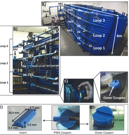
[image:5.612.42.476.74.528.2]Local drinking water (from an upland peat runoff surface water source) was supplied to the facility directly from a cast iron trunk main, trickle fed into an enclosed reservoir tank and re-circulated around the system with a 24 hour retention time, which preserved baseline water quality parameters. Water quality parameters were monitored throughout the experiment (triplicate samples taken weekly, n = 15) and complied with UK standards (S1 Table).
Fig 1. Drinking Water Distribution System (DWDS) simulation pipe facility and Pennine Water Group (PWG) Coupon.A) Test facility, total volume (tank and loops) 4.5 m3, tank volume 1.53 m3, MV = Manual valves used to separate the three loops, 1a, 2a and 3a indicate the 5thcoil of each loop into
which PWG coupons were inserted, 1b, 2b and 3b indicate the 50 mm internal diameter pipes containing flow meters (FM) and control valves; B) Detail of loop arrangement, T = turbidity meter, CV = control valve, other annotations as for A); C) Coupons secured in the apertures; D) HDPE PWG coupon and rubber gasket, to ensure a watertight fit; E) PWG coupon components (insert for microscopy and outer coupon for molecular analyses) and dimensions.
PWG coupons were sonicated with a 2% (w/v) sodium dodecyl sulphate (SDS) solution for 45 minutes and sterile deionised water for 15 minutes, autoclaved [20,21] and inserted into the facility. Before use, the pipe system was disinfected with a 20 mgl-1sodium hypochlorite solu-tion (<16% free chlorine; Rodolite-H, RODOL Ltd, Liverpool, UK) re-circulated within the system for 24 hours, at the maximum achievable flow rate (4.5 ls-1). Subsequently, the system was flushed repeatedly (4.5 ls-1) with fresh water, until chlorine levels decreased to those of the inlet water.
Growth Conditions and Sampling of Biofilm
Biofilms were developed naturally (i.e. no cultures or inoculations were added) for 28 days, at 16°C (± 1°C; controlled and monitored by a cooling unit system), which is representative of water temperatures during summer in the UK. To develop the staining methodology and DIA method, biofilms were established under steady state flows in a pilot run of the experimental system and coupons were sampled at Day 28 (n = 3 per fluorophore, with one coupon per loop). Subsequently, biofilms were developed for physical and microbial community analysis under a steady state flow regime of 0.4 ls-1(shear stress 0.30 Nm-2, Reynolds number*5800). This flow rate is the average recorded in 75–100 mm diameter pipes within UK DWDS [22]. Biofilms were sampled at Day 0 (between 60 and 90 minutes) and Day 28 (n = 9, three per loop, one from each position).
All biofilm samples were collected without draining the system, limiting the impact of sam-pling upon biofilm accumulation, and replacement sterile coupons were immediately inserted into the pipe. Inserts and outer coupons were separated aseptically and used for microscopy (physical structure) and community structure analysis, respectively. It was not feasible to ana-lyse all nine inserts, therefore a subset of five replicates was selected which comprised: a coupon from the crown, middle and invert of loop 2, and a middle coupon from loops 1 and 3. Inserts (n = 5) were fixed in 5% formaldehyde for 48 hours at 4°C and rinsed three times (1 minute washes) in phosphate buffer solution (PBS) containing: 2 mM Na3PO4, 4 mM NaH2PO4,
9 mM NaCl, 1 mM KCl, then stored in PBS at 4°C [23] prior to staining and imaging. Biofilm was removed from all outer coupons (n = 9) by brushing (30 horizontal/vertical strokes) into 30 ml sterile PBS, the resulting suspension was filtered through a 47 mm diameter, 0.22μm pore nitrocellulose membrane (Millipore, MA, USA) using a Microsart membrane filtration unit (Sartorius, UK). Filters were stored at -80°C prior to analysis of microbial community structures via DNA based fingerprinting approaches.
Physical Structure: Biofilm Staining and Fluorophore Combinations
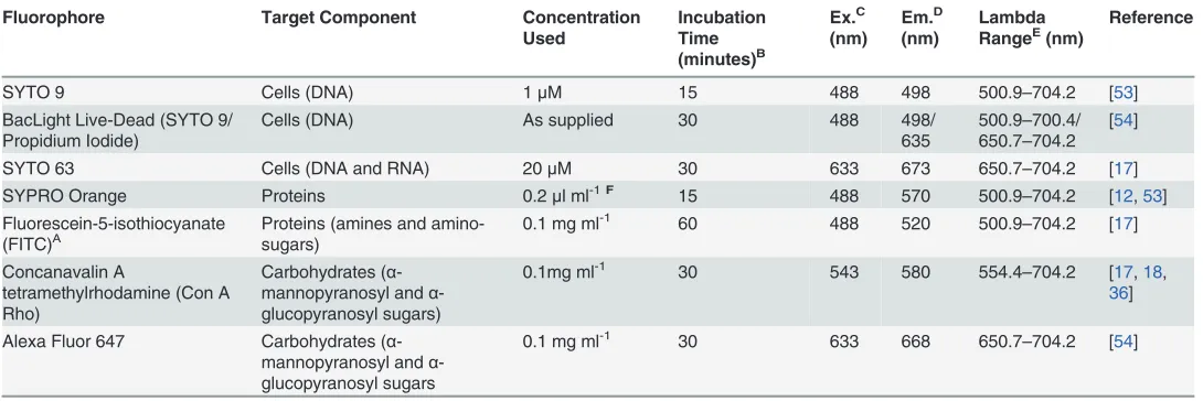
Multiple fluorophores were evaluated for their suitability for use with DWDS biofilm samples, particularly their ability to be resolved from any autofluorescence of the HDPE insert surface, un-stained DWDS biofilm and any signal(s) from other fluorophores. To assess this, fluorophores (Table 1) targeting different biofilm components (nucleic acids, glycoconjugates or proteins/ amines—hereafter referred to as cells, carbohydrates and proteins) were applied singularly, and subsequently, in paired or triple combinations to DWDS biofilms. Fluorophores were selected on the basis of their previous application to microbial aggregates [12,17], their suitability for CLSM analysis and their distinct excitation/emission spectra Although DAPI is frequently used to visualise cells via epifluorescent microscopy [19], this fluorophore was not analysed as no suit-able single photon laser (405 nm) was availsuit-able.application was conducted in two or three stages, following the sequence: cell—protein— car-bohydrate, with three intermediate washing stages (1 minute) using sterile PBS, to ensure that lectins were not stained by the protein fluorophore. Standards on glass slides (n = 3) were test-ed to confirm fluorophore binding specificity. Samples were air dritest-ed (10 minutes) and stortest-ed, in the dark, at 4°C prior to CLSM imaging. It is recognised that air drying may reduce the bio-film volume as desiccation decreases the cytoplasmic volume of cells and the EPS may also ap-pear thinner, due to it being highly hydrated [3]. Consequently, it is preferable to analyse unfixed, hydrated samples but the extensive sampling schedule did not allow for this. Nonethe-less, air drying was minimal and occurred post-fixing so the position of the components was preserved; all the samples were treated identically, therefore results remain comparable.
Physical Structure: Empirical Testing of Fluorophore Combinations via
CLSM
Lambda-Z-Stack Imaging. To analyse cells and EPS throughout the biofilm a LSM510 meta
up-right confocal microscope and LSM510 software (Zeiss, Germany), within the Kroto Imaging Fa-cility (The University of Sheffield, UK) and three single photon lasers (488 nm—argon laser, 543 nm helium/neon laser, 633 nm helium/neon laser) were used to produce lambda-Z-stacks. In brief, a series of XY lambda images (optical slice 4.7μm) were taken at regular intervals (2.35
[image:7.612.35.580.96.278.2]μm; seeS1 Fig.). The Z-stack limits were investigator-selected, therefore, the stack size varied be-tween fields of view (FOV), due to differences in biofilm coverage and the topography of the plastic (S1 Fig.). Samples were secured within a specially designed holder and imaged using a: ×20 EC Plan Neofluar objective (0.5 NA), 420μm2image area, 3.94μs pixel dwell time and 832 × 832 pixels frame size, selected to facilitate detection of a single cell (1 pixel = 0.51μm).
Table 1. Fluorophores (fluorescent stains) evaluated for their use in visualising cells, proteins or carbohydrates within drinking water biofilms.
Fluorophore Target Component Concentration
Used Incubation Time (minutes)B Ex.C (nm) Em.D (nm) Lambda RangeE(nm)
Reference
SYTO 9 Cells (DNA) 1μM 15 488 498 500.9–704.2 [53]
BacLight Live-Dead (SYTO 9/ Propidium Iodide)
Cells (DNA) As supplied 30 488 498/
635
500.9–700.4/ 650.7–704.2
[54]
SYTO 63 Cells (DNA and RNA) 20μM 30 633 673 650.7–704.2 [17]
SYPRO Orange Proteins 0.2μl ml-1F 15 488 570 500.9–704.2 [12,53]
Fluorescein-5-isothiocyanate (FITC)A
Proteins (amines and amino-sugars)
0.1 mg ml-1 60 488 520 500.9–704.2 [17]
Concanavalin A
tetramethylrhodamine (Con A Rho)
Carbohydrates (α -mannopyranosyl andα -glucopyranosyl sugars)
0.1mg ml-1 30 543 580 554.4–704.2 [17,18,
36]
Alexa Fluor 647 Carbohydrates (α -mannopyranosyl andα -glucopyranosyl sugars
0.1 mg ml-1 30 633 668 650.7–704.2 [54]
ABefore staining, samples were pre-washed in 0.1 M sodium bicarbonate, to retain the amines in non-protonated form [36]. BProtected from light.
CExcitation wavelength used in this study, 488 nm-argon laser, 543 nm and 633 nm-helium/neon lasers. DEmission maxima according to supplier(s)
ELambda detection range over which emitted light was collected, the lower boundary was selected to avoid collecting the excitation laser-flare but ensure
the emission peak wavelength was included where possible
FSYPRO Orange molecular weight/molar concentration not provided by supplier, stock stated as 5000× concentration, diluted using 7.5% acetic acid.
Multispectral data stacks (S1 Fig.) with 10.7 nm resolution were obtained, with the settings opti-mised for each stain individually (Table 1). To minimise focal drift, room and sample tempera-tures were allowed to stabilise for 30 minutes prior to imaging and the room temperature was monitored throughout (average 24.6°C ± 1°C) using an EL-USB1 temperature logger (Lescar Ltd., Sailsbury, UK).
Autofluorescence of Controls and Emission Fingerprints.Unstained controls were observed
to auto-fluoresce when exposed to each excitation wavelength (488 nm, 543 nm and 633 nm; see S2 Fig.) but no staining of the plastic was observed. Imaging in lambda mode enables autofluor-escence to be removed from images of stained biofilms via unmixing—if emission fingerprints are known for each of the components within the image. To determine the emission fingerprint of the autofluorescence of the biomass and/or the PWG insert and individual fluorophores, un-stained sterile inserts (n = 3), unun-stained biofilms (n = 3) and single un-stained biofilms (n = 3, per fluorophore) were imaged at seven FOV. All samples were imaged under the settings opti-mised for each fluorophore. For each fluorophore (or control), 21 emission spectra (one per FOV, for each sample) were analysed graphically using the software R v2.15 [24] to assess their similarity. No difference was found between replicate spectra in any instance, therefore the characteristic emission spectrum was assigned (Fig. 2) by plotting all the spectra and se-lecting the median spectrum (for example, inS2 Fig., ROI 1 would be assigned as the emis-sion fingerprint).
Fluorophore Combinations. Lambda-Z-stacks were subsequently generated for dual or
[image:8.612.201.572.75.351.2]tri-ple stained samtri-ples (n = 3 for each combination thereof, 7 FOV). Linear unmixing was applied,
Fig 2. Emission spectra (fingerprints) of the triple stain combination targeting cells (Syto 63), carbohydrates (Con A Rho) and proteins (FITC), at each excitation wavelength.Note that plastic/biofilm autofluorescence is also shown and that the whole spectrum in each case was used in linear unmixing. A) Emission at 488 nm excitation, image settings for FITC; B) Emission at 543 nm excitation, image settings for Con A Rho; C) Emission at 633 nm excitation, image settings for SYTO 63.
using the pre-determined emission fingerprints, to establish the combinations which could (or could not) be separated (S1 Table). Compatible fluorophore pairs were subsequently estab-lished and based upon these, the triple combination of SYTO 63\FITC\Con A Rho, was tested and confirmed as suitable for use in staining the cells/proteins/carbohydrates within the DWDS biofilm samples. There was no difference in the standard deviations of data based on the analysis of seven FOV compared to a randomly selected subset of five FOV (Wilcoxon tests, W9, p>0.05 in all instances). Consequently, a greater number of replicates (n = 5 rather than n = 3) were analysed at fewer FOV (5 rather than 7), resulting in greater replication overall (n = 25 rather than n = 21).
Physical Structure: Triple-stained Biofilms. The triple-stain combination was applied to
Day 0 and Day 28 biofilms (n = 5, FOV = 5 per replicate), which were imaged in lambda mode (S2 Table) and unmixed prior to DIA. Three Z-stacks, each optimised for one of the three fluorophores, were obtained for each FOV and the data relating to the fluorescence of the tar-geted stain was analysed.
Physical Structure: Digital Image Analysis.DIA was applied to unmixed Z-stacks of triple
stained biofilm samples in order to: reduce the image noise (median filtering); generate a threshold; calculate various quantification parameters; overlay, and render unmixed images; and analyse the resultant data. Details of the DIA are presented in the following sections; the authors used a combination of the freely available programs Python v2.7.2 (http://www. python.org) and R v2.15 [24] for this analysis. All of the quantification measures were calculat-ed using unmixcalculat-ed, mcalculat-edian filtercalculat-ed and thresholdcalculat-ed images.
Median Filtering. Images taken using the far red spectra generally yield a considerable
amount of random background noise [17]. Therefore, a 3 × 3 median filter was applied to all unmixed Z-stack image series before thresholding, quantification or visualization was carried out, to maintain a fine level of detail [25].
Thresholds and Area Coverage.Not all stain associated pixels are an exact match to the
fluorophore signal so it is necessary to establish the level at which a pixel associated with the stained component is deemed stain-positive or stain-negative. In this study possible threshold values ranged from 1 to 4095, where a threshold value of 1 would label all of the pixels associat-ed with a particular fluorophore as stain positive (4095 would label none).
The area covered by the stained component was calculated for each image in a Z-stack by di-viding the number of stain associated pixels (at a given threshold) by the total number of pixels in the image (832 × 832). Area coverage (expressed as a fraction) was the principal quantified parameter and a prerequisite for all subsequent DIA; therefore these data were used to inform the selection of a threshold value. In brief, area coverage data were generated for all possible thresholds and normalised by the maximum value in each instance. The data were analysed graphically and statistically [Kruskal Wallis Test;24] to determine the range of thresholds be-tween which there was no difference in the normalised data. The median was chosen as the threshold value for each fluorophore, namely: SYTO 63 (cells) threshold 2401, Con A Rho (car-bohydrates) threshold 1701, and FITC (proteins) threshold 1701. The pitfalls of thresholding are well acknowledged [26] but selecting a threshold in this way removes any investigator-bias and individual FOV influences, which standardises the process, facilitating comparison between datasets.
Volume and Composition.In order to quantify and characterise the composition of the
drinking water biofilms, the volume (μm3) of each of the stained components was generated using the equation:
Volume¼dZ
2 ImageAreaTotal
Xb
i¼a
Where optical slice depth (dZ) is 4.7μm,ImageAreaTotalis 420μm2,ais thefirst slice of the
Z-stack,bis the last slice andAreaCoverageFractionis the proportion of the slice covered by the particular stain for which volume is being calculated. The volume was relative to the minimum detection threshold applied previously, but will be referred to solely as“volume”. Subsequently, the volumes of EPS (protein plus carbohydrate) and total biofilm (EPS plus cells) were calculat-ed and the biofilm composition was evaluated by generating ratios of carbohydrate-to-protein, carbohydrate-to-cells and protein-to-cells.
Distribution and Spread (Thickness).It was desirable to compare the area covered by
cells, carbohydrates or proteins throughout the biofilm. However, this was not possible because the stack size differed with each FOV. Therefore, FOV were normalised by labelling the slice with maximum coverage of cells as slice“0”and numbering slices above and below consecu-tively. The cells were chosen as the component to align to because they produce the EPS and, in physical extraction EPS analysis, the EPS quantity is commonly related back to cell abundance.
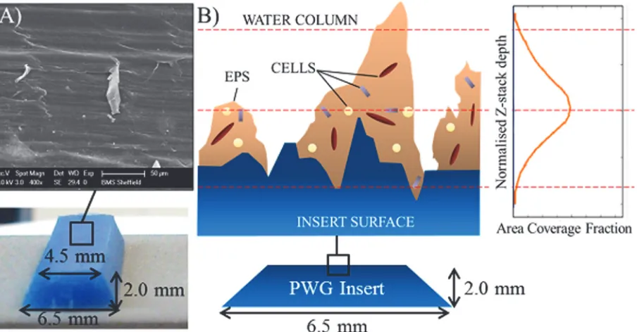
Normalised Z-stack depth was calculated by multiplying the aligned slice number by the thickness (4.7μm) of each slice, this was plotted against area coverage, producing area distribu-tion plots, a schematic example of which is shown inS1 Fig.Note that the y-axis of the area dis-tribution plots runs from positive values which correspond to the biofilm-plastic interface (i.e. the bottom of the biofilm) to negative values which correspond to the biofilm-bulk water inter-face (i.e. the top of the biofilm). It should be recognised that the low area fractions at the bor-ders of the biofilm-plastic interface are considered to be due to the uneven surface of the plastic insert (Fig. 3).
Area distribution plots were compared visually and the aligned slice number with the maxi-mum area coverage recorded for each component—termed the“peak location”. As the Z-stacks were aligned using the cells, their peak location was always zero. However, the peak location of the carbohydrates and proteins could occur on any slice.
Biofilm thickness is often calculated based on the assumption that the biofilm spans the whole Z-stack and that no biofilm exists outside the Z-stack range. In reality, the first and last slides of a Z-stack tend to contain little material. Consequently, biofilm thickness is likely to be overestimated if calculated in this way, unless a second threshold is applied. To avoid this, a pa-rameter termed“spread”(μm) was defined, as a proxy for thickness:
Spread¼ Volume
AreaCoveragePeakImageArea Equation 2
This enabled the distinction between differently shaped area distribution plots (S1 Fig.) as broader distributions have higher spread values.
Statistical Analysis.The volume, spread and peak location data were not normally
distrib-uted (Shaprio Wilks Test, p<0.05), therefore, all quantification was based upon the range and median; significance was tested with the Wilcoxon two-sample test (for which W and p values are presented).
Biofilm Visualisation.The median filtered, thresholded data for each slice within the three
Microbial Community Structure Analysis
DNA Extraction. DNA was extracted from the nitrocellulose filters from Day 0 and Day 28
samples (n = 9) and negative controls (n = 3), using the proteinase K chemical lysis method [27]. Briefly, filters were incubated with 720μl of SET buffer (0.75 M sucrose, 40 mM EDTA, 50 mM Tris-HCl, pH 9) and 81μl of lysozyme (10 mgml-1), at 37°C for 30 minutes with rota-tion in a hybridizarota-tion oven (Thermo Scientific, UK). A 90μl volume of 10% SDS (w/v) and 25μl volume of proteinase K (20 mgml-1; Applied Biosystems, UK) were added, prior to incu-bation for a further 2 hours (with rotation) at 55°C. The resultant lysate was added to 137μl of 5 M NaCl and 115μl of 1% CTAB (hexadecyltmethyl ammonium bromide)/ 0.7 M NaCl solu-tion and incubated (with rotasolu-tion) at 65°C for 30 minutes. The upper aqueous layer was trans-ferred to a clean tube and an equal volume of chloroform/isoamyl alcohol (24:1) added, prior to being centrifuged for 5 minutes—note that all centrifugation was at 12,000 xg. DNA was pre-cipitated with 815μl of 100% isopropanol at -20°C, for 12–14 hours, before centrifugation for 30 minutes. The DNA pellet was washed twice with 70% ethanol, dried and eluted in 30μl of sterile nuclease free water (Ambion, Warrington, UK).
PCR Amplification. DNA extracts were used as templates for three different PCR
amplifi-cations (carried out on an AB 2720 thermal cycler (Applied Biosystems, Warrington, UK) for specific gene fragments from bacteria (16S rRNA), archaea (16S rRNA) and fungi (ITS region). Each PCR was carried out using the conditions and primer pairs shown inTable 2. The for-ward primer was labelled with 6’carboxyfluorescein dye (6-FAM) to enable detection via fluo-rescent fingerprint analysis. Bacterial PCR consisted of 12.5μl of Sigma ReadyMixTaq
[image:11.612.40.492.78.314.2]solution (Sigma Aldrich, UK), 0.4μM of each oligonucleotide primer and 2μl of DNA tem-plate, in a final volume of 25μl. Archaeal PCR consisted of 1 × reaction buffer, 10μl of Q-solu-tion, 100μM dNTPs, 0.15μM of each oligonucleotide primer, 1.25 U ofTaqDNA polymerase
Fig 3. Explanation for the area distribution shape given the uneven surface of the insert.A) Scanning electron microscope image showing the uneven surface of a sterile insert; B) Schematic of the uneven insert surface with biofilm growth, HDPE roughness height is commonly taken in modelling to be 20μm, 80μm was the greatest depth measured in Day 28 biofilms. Broken red lines indicate parts of an example area distribution curve and the corresponding cut through position of the biofilm.
(Qiagen, Crawley, UK) and 1–2μl of DNA template, in a final volume of 50μl. Fungal PCR contained 1 × reaction buffer, 1 mM MgCl2, 50μM dNTPs, 0.2μM of each oligonucleotide
primer, 2.5 U ofTaqDNA polymerase (Qiagen, Crawley, UK) and 1–2μl of DNA template, in a final volume of 50μl. PCR products were confirmed by agarose gel electrophoresis and puri-fied using the QIAquick PCR purification kit (Qiagen, Crawley, UK).
Community Fingerprinting. Two fingerprinting techniques were applied; bacterial and
ar-chaeal communities were analysed using terminal-restriction fragment length polymorphism (T-RFLP) [28,29], fungal communities were analysed using Automated Ribosomal Intergenic Spacer Analysis (ARISA) [30]. Purified bacterial and archaea 16S rRNA amplicons were di-gested separately with 10 U AluI (Roche, Germany) in a total volume of 15μl, at 37°C for 2 hours.
Aliquots (5μl) of the digested bacteria or archaea PCR products, or the purified undigested fungal PCR products were desalted via precipitation with 0.25μl of glycogen (20 mg ml-1; Fer-mentas Thermo Scientific, Loughborough, UK) and 0.53μl of sodium acetate (3 M, pH 5.2) in 70% ethanol (centrifuged at 4°C, for 20 minutes). The pellet was washed twice in 70% ethanol and re-suspended in 5μl of nuclease free water (Ambion, Warrignton, UK).
Desalted bacterial or archaeal digests were denatured with hi-di formamide containing 0.5% GeneScan 500 ROX internal size standard (Applied Biosystems, Warrington, UK), in a total volume of 10μl. Desalted fungal amplicons were combined with hi-di formamide containing 0.5% ROX GeneScan 2500 internal size standard (Applied Biosystems, Warrington, UK), in a total volume of 10μl. Samples (and internal size standard controls) were denatured at 94°C for 3 minutes, cooled on ice and electrophoresed using an ABI 3730 PRISM capillary DNA analy-ser using POP7 (denaturing) polymer (Applied Biosystems, Warrington, UK) at injection times of 5, 10 or 20 seconds, with an initial injection voltage of 2 kV, followed by ten incremen-tal voltage increases (each 20 seconds) to a final run voltage of 15 kV. The toincremen-tal electrophoresis run was 20 minutes for T-RFLP and an hour for ARISA.
Community Composition Data Analysis. The resulting T-RFLP and ARISA
[image:12.612.37.578.105.275.2]electrophero-grams were analysed via GeneMapper v3.7 (Applied Biosystems) to establish the size of each
Table 2. Oligonucleotide primer pairs used to amplify 16S rRNA genes and ITS regions, PCR cycling conditions used in each case are indicated.
Microorganism (amplified gene)
Amplicon Size (nt)
Oligonucleotide PrimersA PCR Cycle Conditions Ref.C
Primer Pair Primer Sequence (5’–3’) Temperature (°C) and Duration
(minutes:seconds)
CyclesB
Bacteria (16S rRNA)
*455 FAM-63F and 518R
6-FAM-CAGGCCTAACACATGCAAGTC and CGTATTACCGCGGCTGCTCG
Initial denaturation 94°C, 2:00; Denaturation 94°C, 0:30; Annealing 55°C, 0:30; Elongation 72°C, 0:45; Elongation stop 72°C, 10:00
×30 [55]
Archaea (16S rRNA)
*849 FAM-Arch109F and Arch958R
6-FAM-ACKGCTCAGTAACACGT and YCCGGCGTTGAMTCCAATT
Initial denaturation 95°C, 0:45; Denaturation 95°C, 0:45; Annealing 55°C, 1:00; Elongation 72°C, 1:30; Elongation stop 72°C, 10:00
×35 [56]
Fungi (ITS region) *200–1000 FAM-ITS1F and ITS4
6-FAM—
CTTGGTCATTTAGAGGAAGTAA and TCCTCCGCTTATTGATATGC
Initial denaturation 95°C, 5:00; Denaturation 95°C, 0:30; Annealing 55°C, 0:30; Elongation 72°C, 1:00; Elongation stop 72°C, 10:00
×35 [46]
AAll primers were sourced from Sigma, UK
BNumber of cycles of the denaturation, annealing and elongation steps CReferences that used these primer combinations.
T-RF (50–500 nucleotides) or ARISA fragment (94–827 nucleotides), as estimated using the Local Southern method (in comparison with the internal size standards). To remove noise, only T-RF/ARISA peak heights greater than 50 fluorescent units were analysed. Fingerprint profiles were expressed in terms of the peak area and size of each T-RF/ARISA fragment and aligned using T-Align [31], with a confidence interval of 0.5 nt. Aligned data was normalised to exclude terminal-restriction fragments (T-RFs) or ARISA fragments that contributed<0.5% to the community profile. Normalised datasets were square root-transformed and Bray-Curtis similarity matrices were generated [32] to compare the relative abundance of T-RFs/ARISA fragments in each profile. Multivariate analysis was carried out using PRIMER-E v6.1 [32]; spe-cifically, hierarchical clustering with similarity profile assessment (SIMPROF; 20,000 permuta-tions), analyses of similarity (ANOSIM) tests (for which global R and p values are presented) and similarity percentage calculations (SIMPER). Three ecological indices, relative to the com-munity profile [33], were calculated: richness (i.e. the total number of T-RFs/ARISA fragments per sample), Shannon’s diversity index [34] and Pielou’s evenness index [35]. T-tests were per-formed to assess significance, for which degrees of freedom (df) and p values are presented.
Results
Characterizing Biofilm Physical Structure
Position Effects.Analysis of the position of the coupon within the loop or the loop number
showed no significant difference with respect to the volume (W>79.5, p>0.0590 and<0.9834) or spread (W>96.5, p>0.1644 and<0.7873) of cells, carbohydrates or proteins. Similarly, there was no significant difference in the peak location of carbohydrates (W113.0, p0.2161) or proteins (W88.5, p0.0856), indicating that there was no influence of position upon bio-film physical structure. Consequently, all subsequent analysis of biobio-film images, from a given time point, used the data set as a whole (n = 25).
Visualisation and Characterisation of DWDS Biofilms after 28 Days of Growth.After
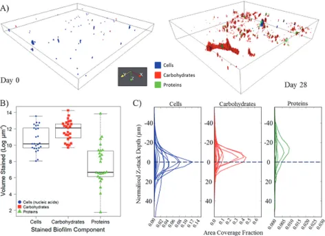
28 days of growth, biofilms were heterogenic in their coverage and morphology (e.g.Fig. 4A). A FOV generally contained all three stained components but no complete co-localisation was observed; the extent of carbohydrate coverage in contrast to that of proteins was illustrated, along with areas where either only cells or EPS were present. The median total biofilm volume at Day 28 was 252325μm3(per 420μm2FOV), of which carbohydrates were the dominant component (Fig. 4;Table 3) occurring at a significantly greater volume than either cells (W = 179.0, p = 0.0090), or proteins (W = 40.0, p<0.0001). Proteins occurred at a significantly lower volume than the cells (W = 543.0, p<0.0001) and were consistently the least abundant biofilm component (Fig. 4;Table 3). The range in volume of each of the components (Table 3) indi-cates the substantial heterogeneity in biofilm coverage and supports the choice of analysing a greater number of sample replicates.
Although some biofilm material was visualised at Day 0 (Fig. 4A), this was uneven and thin-ly dispersed, compared to Day 28 biofilms. As expected, the total volume of biofilm at Day 0 (Table 3) was significantly lower than that at Day 28 (W = 77, p<0.0001). In contrast to Day 28 biofilms, Day 0 material was predominantly comprised of cells with little or no EPS detected (Table 3); proteins were particularly sparse or absent completely at Day 0 (e.g.Fig. 4A). Each of the three stained components had a greater volume at Day 28 compared to Day 0 but, despite a 47-fold increase in the minimum cell volume and a five-fold increase in the maximum
Conversely, the carbohydrate-to-cell ratio increased significantly from 0.31 at Day 0 to 4.80 at Day 28 (W = 151.0, p = 0.0014).
[image:14.612.39.511.77.420.2]All stained components within a Day 28 biofilm occurred throughout a similar normalised Z-stack depth (Fig. 4C), i.e. they were present on a similar number of Z-stack slices. This obser-vation was supported by the similarities (W318, p0.2389) in spread values for cells (median = 25.70μm), carbohydrates (median = 24.91μm) and proteins (median = 26.30μm). Although the three components were present across similar depths of biofilm, the areas which they covered at each depth varied considerably, with the protein area coverage fraction generally one or two orders of magnitude lower than cells or carbohydrates, respectively (Fig. 4C). Commonly, the peak area fractions of the carbohydrates and proteins occurred above that of the cells (i.e. closer to the bulk water). This can be seen inFig. 4Cfor Day 28 biofilms, where the peak of the carbo-hydrate or protein area distributions occurs above the peak of the cells by an average of 1 or 3 slices, respectively. This trend was also seen at Day 0, with no significant difference in the peak
Fig 4. An example of the arrangement, volume and distribution of cells, carbohydrates and proteins of drinking water biofilms.A) 3D projection of example Day 0 and Day 28 biofilms, plotting region shown is 420μm × 420μm × 30.6μm and 420μm × 420μm × 94.4μm, respectively; B) Volume (log) of biofilm components at Day 28, relative to the thresholds used in digital image analysis, each data point (n = 25) represents a FOV, box and whisker plots show the range, interquartile range and median—indicated by the solid black line; C) Day 28 area distribution plot, each line (n = 25) indicates a FOV, note the different x-axis scales between components. Area coverage fraction refers to the proportion of each XY image of the Z-stack covered by the particular component, blue dashed line at“0”indicates the cell peak location; peak location is the aligned slice number at which the maximum area fraction occurs. Area fractions for carbohydrates and proteins are plotted relative to cells (seeMaterials and Methodsfor details).
location of the EPS molecules (in relation to the peak location of the cells) between Day 0 and Day 28 biofilms (carbohydrate, W = 233.5, p = 0.1459; protein, W = 323.0, p = 0.5677).
Biofilm Microbial Community Structure
Position Effects.The position or loop from which coupons were sampled did not alter the
community structure with respect to bacteria (ANOSIM: global R<0.00, p0.626), archaea (ANOSIM: global R<0.00, p0.828) or fungi (ANOSIM: global R0.12, p0.152), in either Day 28 or Day 0 biofilms. Therefore, there was no requirement to account for differences in coupon location in subsequent community structure analyses.
Characterisation of DWDS Biofilms after 28 Days of Growth.Bacteria, archaea and fungi
were detected in all nine biofilm samples from Day 28 but the archaeal communities had a re-duced relative richness compared to the bacterial and fungal communities (Table 4). According to a search of known and“uncultured”archaea in the Ribosomal Database Project (rdp.cme. msu.edu), a total of 307 T-RFs ranging from 2 nt to 500 nt in size, are possible with the primer/ enzyme combination used. Therefore low archaeal diversity was not due to a conserved region across different archaea species but a true reflection of the small number of taxa identified within Day 28 drinking water biofilms.
[image:15.612.35.580.95.257.2]Fewer microbial PCR products were amplified from Day 0 biofilms (2/9 bacterial, 5/9 ar-chaeal and 5/9 fungal PCR products) compared to Day 28 biofilms (9/9 in all instances). As bacteria were only detected in 2 samples from Day 0, it was not appropriate to calculate an av-erage of the ecological indices or undertake statistical comparison to Day 28 data, instead the minimum and maximum values were compared and the trends reported. Overall, microbial communities were more complex at Day 28 than at Day 0, with significantly greater relative taxon richness for archaea (df = 5.15, p = 0.0441) and fungi (df = 11.61, p = 0.0353) (Table 4). However, no significant difference in relative diversity was detected in any of the biofilm mi-crobial communities (df4.68, p0.1125 and relative evenness did not differ in the bacterial or fungal communities (df = 11.75, p = 0.8039). Conversely, archaeal communities at Day 28 had
Table 3. Volumes and ratios of the stained cells, carbohydrates and proteins of drinking water biofilms.
Component Range (Minimum—Maximum) Median
Volume (μm3) Day 0 Day 28 Day 0 Day 28
Cells 66–137860 3119–769191 35543 26099
Carbohydrates 1–189129 16257–1537181 9874 180802
Proteins 0–1387 6–1027266 177 800
EPSA 29–189132 16518–1545084 11059 184850
Total BiofilmB 321–261128 31268–2085836 50745 252325
Volume RatiosC Day 0 Day 28 Day 0 Day 28
EPS: Cells 0.0–112.9 0.1–152.7 0.4 4.9
Carbohydrates: Cells 0.0–112.3 0.1–151.9 0.3 4.8
Proteins: Cells 0.0–0.5 0.0–2.5 0.0 0.1
Carbohydrates: Proteins 0.0–80480.5 0.3–36889.2 46.8 62.3
AEPS = Carbohydrates + Proteins, before averaging
BTotal Biofilm = Cells + Carbohydrates + Proteins, before averaging. In both instances, data presented are therefore the minimum, maximum and median
of the sums
CThefirst component is divided by the second; a value>1 indicates a greater volume of thefirst component; a value<1 indicates a greater volume of
the second component.
a significantly lower relative evenness value than those at Day 0 (df = 6.50, p = 0.0327), indicat-ing the dominance of certain T-RFs at Day 28.
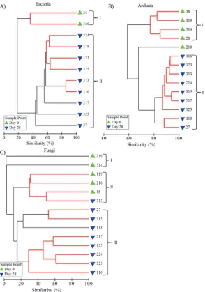
Comparisons of microbial community structure at each sample point demonstrated that, for each microbial group, Day 28 profiles clustered independently from those of the Day 0 biofilms (Fig. 5) and contained significantly different compositions of T-RFs (bacteria, glob-al R = 1.0000, p = 0.0018; archaea, globglob-al R = 0.822, p = 0.0005) or ARISA amplicons (globglob-al R = 0.593, p = 0.0005). With respect to bacteria and archaea two distinct clusters were ob-served, with the exception of one replicate (210) in the archaeal community analysis which did not cluster with the communities present in Day 0 biofilm samples (cluster I) or with the biofilm communities present at Day 28 (cluster II,Fig. 5). Fungal community profiles formed three clusters (Fig. 5), the second of which incorporated Day 0 samples and one Day 28 sample (replicate 313). However, when analysed by presence/absence rather than relative abundance, all replicates from Day 0 clustered independently from those from Day 28, sug-gesting that the same ARISA amplicons were dominant between the samples in cluster II but that there was a difference in the richness of ARISA fragments between the two time points.
[image:16.612.35.578.106.216.2]Little variation existed between replicates (Table 4) with the greatest variation occurring between fungal community profiles. Nevertheless, profiles were often indistinguishable from at least one other profile from the same sample point, assessed by SIMPROF (indicated by the red lines inFig. 5). The fungal community profiles were also the most heterogenic be-tween Day 0 and Day 28 biofilms (average similarity 7.35%), followed by the bacteria (18.21%) and archaea (61.56%) communities. Analysis of the T-RFs/ARISA amplicons which accounted for the majority (60%) of the differentiation between the Day 0 and Day 28 biofilm communities demonstrated that some T-RFs or amplicons were unique to Day 0 samples and that 16 bacterial T-RFs, 1 archaeal T-RF and 7 fungal ARISA amplicons were only present at Day 28.
Table 4. Ecological diversity indices and similarity values of the bacterial, archaeal and fungal communities from drinking water biofilms sampled at Day 0 and Day 28.
Sample Point Microbialfingerprint Relative RichnessB Relative EvennessD Relative DiversityE Similarity between replicates (%)F
Mean (St.Dev.)C Mean (St.Dev.)C Mean (St.Dev.)C
Day 0 BacteriaA 3 & 5 0.89 & 0.95 1.04 & 1.43 36.30
Archaea 8 (2.39) 0.92 (0.02) 1.90 (0.28) 66.54
Fungi 11 (5.76) 0.91 (0.03) 2.05 (0.61) 9.75
Day 28 Bacteria 37 (4.59) 0.97 (0.01) 3.48 (0.13) 52.83
Archaea 11 (1.20) 0.89 (0.01) 2.15 (0.11) 85.80
Fungi 24 (13.51) 0.91 (0.06) 2.77 (0.67) 25.38
An = 2 therefore no average could be calculated, both values are presented BNumber of T-RFs
CStandard deviation DPielou's Index EShannon's Index FSIMPER analysis.
Discussion
[image:17.612.202.496.76.495.2]A triple staining, CLSM imaging and novel DIA protocol was established by empirical testing and applied, for the first time, to concurrently visualise and quantify cells, carbohydrates and proteins of biofilms from a full-scale DWDS facility. It is recognised that fluorophores applied to target cells will stain extracellular DNA (eDNA) as well as intracellular DNA, however, eDNA has been reported at very low concentrations in EPS and, if present, is likely to be in concentrations below the limit of detection of staining methods [16]. The above combination of stains was previously used to investigate the EPS of aerobic granules from a bioreactor fed with synthetic wastewater and sludge [36]. However, herein, this fluorophore combination has been applied to characterise microbial biofilms that develop naturally upon the surface of an
Fig 5. Cluster analysis of similarity using fingerprint profiles to show the similarity between A) bacterial, B) archaeal and C) fungal drinking water biofilm communities.Relative abundance data was derived from T-RFLP or ARISA analysis, sample identification numbers are shown and clusters are indicated with a bracket and number. Red lines indicate profiles not significantly dissimilar according to SIMPROF analysis.
engineered, chlorinated DWDS system, with an oligotrophic environment contrasting consid-erably from that of wastewater. A novel advance in the DIA approach has enabled quantitative analysis of each biofilm component, incorporating a method to establish biofilm“thickness” which is unaffected by the uneven scaffold of the internal DWDS pipeline plastic surface and is independent of the potential biases caused by investigator-selection of the Z-stack limits.
Previously, the process of material accumulation at the pipe wall of a DWDS has been re-ferred to as gravity-driven sedimentation of suspended particles, which may subsequently be re-suspended causing water quality issues such as discolouration [37,38]. Boxallet al. [39] sug-gested an alternative hypothesis, that material accumulates at the pipe wall in“cohesive layers”, adhered via particle-pipe interactions, in layers of different strengths, which detach when the shear stress exceeds that experienced during accumulation; a concept validated by field and laboratory studies [22,40] and analogous to the formation and detachment of microbial bio-films, more broadly. If gravity-driven sedimentation is the main driver in biological material formation within DWDS, a difference would be expected between biofilms from the invert of the pipeline in comparison to those from the crown. However, there was no significant spatial variation in biofilm physical characteristics or community structure between locations around the internal circumference of the pipe. Where variation between replicates was observed this was attributed to the heterogenic nature of biofilms, and their stochastic development [41]. Therefore, we conclude that the cohesive layer theory better represents the accumulation of bi-ological material within the context of DWDS than gravity-driven sedimentation. This is in contrast to wastewater networks, where material does accumulate to a greater degree on the in-vert of the pipeline and comprises bacterial communities distinct from those at the crown [42]. At Day 28 the volume of each stained component increased compared to Day 0, as did the EPS-to-cell ratio, indicative of the development of a more mature biofilm, producing an EPS matrix to adhere to the substrata, consistent with previous studies which identified EPS as the main biofilm component [3,14]. Within a wastewater inoculated biofilm developed at a Rey-nolds number of 4000, the quantified EPS (carbohydrates only) and cells were shown to in-crease over 31 days but no significant difference in the EPS-to-cell ratio was reported [12]. It is possible that the switch in dominance of EPS over cells, observed here in biofilms within a chlorinated drinking water system, is due to the need for a greater protection of the cells from a more challenging environment (e.g. oligotrophic, higher disinfectant residuals) than that of the wastewater conditions investigated by Wagneret al. [12].
In the present study, the EPS within DWDS biofilms was consistently dominated by carbo-hydrates; generally, proteins were found in volumes lower than that of the cells. Analysis of the proteins in comparison to carbohydrates within DWDS biofilms is rare but such comparisons exist in biofilms from other environments, such as activated sludge flocs, where proteins were more common than carbohydrates [11] or inPseudomonas fluorescensbiofilms cultured within a reactor, in which carbohydrate was the dominate EPS component [14]. Although, in the latter example, the EPS was studied via extraction based methods rather than fluorescent microsco-py. Raman microscopy and CLSM analysis of cell/carbohydrate and cell/protein stained bio-films cultured within a wastewater sludge seeded reactor also found carbohydrate to be the most abundant EPS component while proteins could not be detected in biofilms younger than 31 days [12]. In contrast, this study has shown that protein is present in DWDS biofilms at de-tectable quantities, albeit at lower volumes than cells or carbohydrates. The consistent predom-inance of carbohydrates reported in the literature, for biofilms from different growth
contain particularly high amounts of carbohydrate in the basal layer, which was found to be more stable than the biofilm at the surface.
Cells, carbohydrates and proteins exhibited a similar spread but were not uniformly distrib-uted throughout the biofilm, nor did the different biofilm components completely co-localise. The results presented herein enabled, for the first time, comparison of the arrangement of cells, carbohydrates and proteins throughout a cross section of a DWDS biofilm, in relation to each other. The differential location of the cells, carbohydrates and proteins was observed, including regions covered solely by cells or one of the EPS molecules, a trend also highlighted by Stewart
et al. [44], with respect to cells and carbohydrates. While the presence of cell free areas where EPS is observed could be due to the cell volume being below the limit of detection, it seems more likely that these EPS regions represent sites from which cells have migrated, been de-tached or lysed. The different location of the EPS throughout the three-dimensional structure of the biofilm, and in relation to the cells, has not been extensively considered in the literature. However, within wastewater-fed biofilms a greater cell concentration was reported nearer to the surface in contact with the bulk phase, attributed to a better nutrient and oxygen supply [12] but no analysis of EPS distribution was presented. In contrast, this study has established that the peak location of the EPS within biofilms from a chlorinated DWDS was nearer to the biofilm-water interface than the cells. Potentially, as microorganisms produce EPS, the mole-cules may be preferentially secreted above the cells to form a barrier protecting against the po-tentially harmful physico-chemical stresses (e.g. shear forces, disinfectant residual) imposed by the water phase.
In addition to variation in physical structure between Day 0 and Day 28, the biofilms also experienced a change in microbial community structure; the bacterial, archaeal and fungal rela-tive richness increased during the development phase, although the archaeal communities were less complex than the bacterial or fungal communities. Previous drinking water studies have focused upon bacteria [5,6] or fungi [45]. In contrast, there had been limited research considering archaea in DWDS due in part to the historical difficulties in culturing these micro-organisms and that most studies focus solely on one taxonomic domain, typically bacteria. Of those studies which have looked for archaea, some have concluded that they could not be de-tected [46] while others have confirmed their presence [47]. However, these studies have been based upon samples taken from bench-top systems or taps rather than biofilms from within pipelines, as has been possible with the experimental system presented here. Biofilm studies from environments other than DWDS also found bacterial diversity to be greater than that of archaea [48]. A review of a range of microbial community studies from an array of environ-ments established that reduced archaeal diversity is inherent across various habitats [49]. Ar-chaeal communities may be less diverse than bacteria due to different interactions with the environment, potentially expressing less physiological flexibility. Interestingly, around two thirds of the archaeal libraries (16S rRNA gene) assessed consisted of rare phylotypes, the same proportion as seen in bacterial libraries [49]. This highlights the importance of archaea, which have not been widely investigated, particularly in the drinking water environment where the major focus is bacteria. The identification of several archaeal T-RFs and fungal ARISA ampli-cons demonstrated in the present study further highlights their role as an important, quantifi-able part of the microbial community within DWDS biofilms.
water biofilm [52]. In combination with the results presented herein, it seems that bacterial successional colonisation in DWDS is plausible and fungal and archaeal communities may ex-perience this also.
Conclusion
The novel, full-scale experimental system and analyses presented herein, provide a detailed ap-proach to characterize the structure of drinking water biofilms formed under real-world condi-tions (hydraulics, physico-chemistry and microbiology). The CLSM and DIA applied are sufficiently sensitive for use in analysing drinking water biofilms and enable characterisation of biofilm physical structure across a variety of parameters. Furthermore this research presents a unique integration of physical (microscopy based) and microbial community structure assess-ment of DWDS biofilms. Application of the method showed that, within 28 days old biofilms, cells accounted for a smaller proportion of the biofilm than EPS and that the microbial fraction was comprised of bacterial, archaeal and fungal communities. Carbohydrates were the predom-inant component, although proteins were detected, and the greatest coverage of EPS occurred above that of the cells. Biofilm physical composition or community structure was unaffected by the position around the circumference of the pipe, demonstrating the role of microorganisms in material accumulation within chlorinated DWDS. Overall, this approach has provided a novel insight into the microbial community structure, EPS matrix structure, composition and the architecture of multi-species biofilms. The analysis approach provides an opportunity to investigate the impact of environmental variation upon the structure of biofilms from DWDS and may be applied across an array of engineered systems (e.g. waste water networks, dental waterlines, jet fuel supply lines). Such application will enable new understanding of biofilms, their roles and interactions with the infrastructure and water phase, ultimately aiding biofilm management, which within the context of DWDS will enable the provision of a safe water sup-ply into the future.
Supporting Information
S1 Fig. Schematic representation and analysis of lambda-Z-stack data produced via
confo-cal laser scanning microscopy.A) Schematic of a lambda(λ)-Z-stack comprised ofxyλ
im-ages/slices taken at different focal depths (Z) throughout the sample, with an optical slice depth of 4.7μm (i.e. slice thickness for which light is collected); B) Detail of the optical interval (2.35μm) between adjacent slices; C) An exampleλ-Z-stack gallery showing the determination of an emission signal. Example shown is based on excitation at 633 nm, emission collection over 650.7–704.2 nm, into five bins, 10.7 nm wide; midpoint values of the bins are shown in the lambda and Z dimensions. D) Hypothetical area distributions plots, with either the same vol-ume (V) or“area coverage peak × image area”(P) values; spread values (μm) overlaid, spread calculated usingEquation 2(see text for details).
(TIF)
S2 Fig. Auto-fluorescence of the unstained controls, with excitation at 488 nm.A) Example
of the unstained plastic and biofilm compared to a FITC stained sample, scale bar 100μm; B) Seven unstained biofilm emission spectra, imaged using FITC settings (488 nm excitation); In-tensity measured in arbitrary units, ROI = region of interest, which refer to the seven FOV. (TIF)
S1 Table. Fluorophore combinations tested with the drinking water biofilm samples in this study.
(DOC)
S2 Table. Final (optimised) Confocal Laser Scanning Microscope settings used to image tri-ple stained drinking water biofilms.
(DOC)
Author Contributions
Conceived and designed the experiments: KEF JBB AMO. Performed the experiments: KEF RLS ID NHG. Analyzed the data: KEF RC. Contributed reagents/materials/analysis tools: AMO JBB NHG. Wrote the paper: KEF JBB NHG AMO RC RLS ID.
References
1. Gauthier V, Barbeau B, Millette R, Block J, Prvost M (2001) Suspended particles in the drinking water of two distribution systems. Water Supply 1: 237–245.
2. Costerton J, Lewandowski Z Z, Caldwell D, Korber D, Lappin-Scott H. (1995) Microbial Biofilms. Annu Rev Microbiol 49: 711–745. PMID:8561477
3. Neu T, Lawrence J (2009) Extracellular polymeric substances in microbial biofilms. Microbial Glycobiol-ogy: Structures, Relevance and Applications. Elsevier, San Diego. pp. 735–758.
4. Denkhaus E, Meisen S, Telgheder U, Wingender J (2007) Chemical and physical methods for charac-terisation of biofilms. Microchim Acta 158: 1–27.
5. Yu J, Kim D, Lee T (2010) Microbial diversity in biofilms on water distribution pipes of different materials. Water Sci Technol 61: 163–171. doi:10.2166/wst.2010.813PMID:20057102
6. Revetta R, Pemberton A, Lamendella R, Iker B, Domingo J (2010) Identification of bacterial populations in drinking water using 16S rRNA-based sequence analyses. Water Res 44: 1353–1360. doi:10.1016/ j.watres.2009.11.008PMID:19944442
7. Douterelo I, Husband S, Boxall JB (2014) The bacteriological composition of biomass recovered by flushing an operational drinking water distribution system. Water Res 54: 100–114. doi:10.1016/j. watres.2014.01.049PMID:24565801
8. Abe Y, Skali-Lami S, Block J-C, Francius G (2012) Cohesiveness and hydrodynamic properties of young drinking water biofilms. Water Res 46: 1155–1166. doi:10.1016/j.watres.2011.12.013PMID:
22221338
9. Stoodley P, Cargo R, Rupp CJ, Wilson S, Klapper I (2002) Biofilm material properties as related to shear-induced deformation and detachment phenomena. J Ind Microbiol Biot 29: 361–367. PMID:
12483479
10. Martiny AC, Jørgensen TM, Albrechtsen H-J, Arvin E, Molin S (2003) Long-term succession of structure and diversity of a biofilm formed in a model drinking water distribution system. Appl Environ Microbiol 69: 6899–6907. PMID:14602654
11. Schmid M, Thill A, Purkhold U, Walcher M, Bottero JY, et al. (2003) Characterization of activated sludge flocs by confocal laser scanning microscopy and image analysis. Water Res 37: 2043–2052. PMID:
12691889
12. Wagner M, Ivleva NP, Haisch C, Niessner R, Horn H (2009) Combined use of confocal laser scanning microscopy (CLSM) and Raman microscopy (RM): Investigations on EPS—Matrix. Water Res 43: 63– 76. doi:10.1016/j.watres.2008.10.034PMID:19019406
13. Jahn A, Nielsen P (1995) Extraction of extracellular polymeric substances (EPS) from biofilms using a cation exchange resin. Water Sci Technol 32: 157–164.
14. Simoes M, Pereira M, Vieira M (2005) Effect of mechanical stress on biofilms challenged by different chemicals. Water Res 39: 5142–5152. PMID:16289205
15. Staudt C, Horn H, Hempel D, Neu T (2004) Volumetric measurements of bacterial cells and extracellu-lar polymeric substance glycoconjugates in biofilms. Biotechnol Bioeng 88: 585–592. PMID:15470707
17. McSwain B, Irvine R, Hausner M, Wilderer P (2005) Composition and distribution of extracellular poly-meric substances in aerobic flocs and granular sludge. Appl Environ Microbiol 71: 1051–1057. PMID:
15691965
18. Shumi W, Lim J, Nam S, Kim S, Cho K, et al. (2009) Fluorescence imaging of the spatial distribution of Ferric ions over biofilms formed byStreptococcus mutansunder microfluidic conditions. Biochip J 3: 119–124.
19. Deines P, Sekar R, Husband P, Boxall J, Osborn A, et al. (2010) A new coupon design for simultaneous analysis of in situ microbial biofilm formation and community structure in drinking water distribution sys-tems. Appl Microbiol Biotechnol 87: 749–756. doi:10.1007/s00253-010-2510-xPMID:20300747
20. Backhus DA, Picardal FW, Johnson S, Knowles T, Collins R, et al. (1997) Soil- and surfactant-en-hanced reductive dechlorination of carbon tetrachloride in the presence ofShewanella putrefaciens 200. J Contam Hydrol 28: 337–361.
21. Buss HL, Brantley SL, Liermann LJ (2003) Nondestructive methods for removal of bacteria from silicate surfaces. Geomicrobiol J 20: 25–42.
22. Husband P, Boxall J, Saul A (2008) Laboratory studies investigating the processes leading to disco-louration in water distribution networks. Water Res 42: 4309–4318. doi:10.1016/j.watres.2008.07.026
PMID:18775550
23. Pawley J (2006) Handbook of Biological Confocal Microscopy. 3rd ed. Available:http://www.springer. com/life+sciences/biochemistry+%26+biophysics/book/978-0-387-25921-5. Accessed 13 February 2014.
24. R Development Core Team (2012) R: A language and environment for statistical computing. Vienna, Austria: R Foundation for Statistical Computing. Available:http://www.R-project.org/.
25. Privett G (2007) Creating and Enhancing Digital Astro Images. 1st ed. Springer-Verlag, London.
26. Yang X, Beyenal H, Harkin G, Lewandowski Z (2001) Evaluation of biofilm image thresholding meth-ods. Water Res 35: 1149–1158. PMID:11268835
27. Zhou J, Bruns MA, Tiedje JM (1996) DNA recovery from soils of diverse composition. Appl Environ Microbiol 62: 316–322. PMID:8593035
28. Liu W.T, Marsh T.L, Cheng H and Forney L.J (1997) Characterization of microbial diversity by determin-ing terminal restriction fragment length polymorphisms of genes encoddetermin-ing 16S rRNA. Appl Env Micro-biol 63: 4516–4522. PMID:9361437
29. Osborn A.M, Moore E.R.B and Timmis K.N (2000) An evaluation of terminal-restriction fragment length polymorphism (T-RFLP) analysis for the study of microbial community structure and dynamics. Env Microbiol 2: 39–50.
30. Ranjard L, Poly F, Mougel C, Thioulouse J, Nazaret S (2001) Characterization of bacterial and fungal soil communities by Automated Ribosomal Intergenic Spacer Analysis fingerprints: biological and methodological variability. Appl Environ Microbiol 67: 4479–4487. PMID:11571146
31. Smith C.J et al (2005) T-Align, a web-based tool for comparison of multiple terminal restriction fragment length polymorphism profiles. FEMS Microbiol Ecol 54: 375–380. PMID:16332335
32. Clarke KR (1993) Non-parametric multivariate analyses of changes in community structure. Aust J Ecol 18: 117–143.
33. Shannon CE (1948) A mathematical theory of communication. Bell Syst Tech J: 379–423.
34. Pielou EC (1966) The measurement of diversity in different types of biological collections. J Theor Biol 13: 131–144.
35. Blackwood CB, Hudleston D, Zak DR, Buyer JS (2007) Interpreting ecological diversity indices applied to terminal restriction fragment length polymorphism data: insights from simulated microbial communi-ties. Appl Environ Microbiol 73: 5276–PMID:17601815
36. Chen M, Lee D, Tay J (2007) Distribution of extracellular polymeric substances in aerobic granules. Appl Microbiol Biotechnol 73: 1463–1469. PMID:17028870
37. Wu J, Noui-Mehidi N, Grainger C, Nguyen B, Mathes P, et al. (2003) Particles in Water Distribution Sys-tem—6th progress report. Particle sediment modelling: PSM software.
38. Vreeburg JHG, Schippers D, Verberk JQJC, van Dijk JC (2008) Impact of particles on sediment accu-mulation in a drinking water distribution system. Water Res 42: 4233–4242. doi:10.1016/j.watres. 2008.05.024PMID:18789809
39. Boxall JB, Skipworth P, Saul A (2001) A novel approach to modelling sediment movement in distribu-tion mains based on particle characteristics. Proceedings of the Computing and Control in the Water In-dustry Conference. DeMonfort University, UK.
41. Wimpenny J, Manz W, Szewzyk U (2000) Heterogeneity in biofilms. FEMS Microbiol Rev 24: 661–671. PMID:11077157
42. Gomez-Alvarez V, Revetta RP, Domingo JW (2012) Metagenome analyses of corroded concrete wastewater pipe biofilms reveal a complex microbial system. BMC Microbiol 12: 122. doi:10.1186/ 1471-2180-12-122PMID:22727216
43. Mohle R, Langemann T, Haesner M, Augustin W, Scholl S, et al. (2007) Structure and shear strength of microbial biofilms as determined with confocal laser scanning microscopy and fluid dynamic gauging using a novel rotating disc biofilm reactor. Biotechnol Bioeng 98: 747–755. PMID:17421046
44. Stewart PS, Murga R, Srinivasan R, de Beer D (1995) Biofilm structural heterogeneity visualized by three microscopic methods. Water Res 29: 2006–2009.
45. Hageskal G, Knutsen AK, Gaustad P, Hoog GS, Skaar I (2006) Diversity and significance of mold spe-cies in Norwegian drinking water. Appl Environ Microbiol 72: 7586–7593. PMID:17028226
46. Manz W, Szewzyk U, Ericsson P, Amann R, Schleifer KH, et al. (1993) In situ identification of bacteria in drinking water and adjoining biofilms by hybridization with 16S and 23S rRNA-directed fluorescent oligonucleotide probes. Appl Environ Microbiol 59: 2293–2298. PMID:8357261
47. Wielen VD, J PWJ, Voost S, Van Der Kooij D (2009) Ammonia-oxidizing bacteria and archaea in groundwater treatment and drinking water distribution systems. Appl Environ Microbiol 75: 4687–4695. doi:10.1128/AEM.00387-09PMID:19465520
48. Fernandez A, Huang S, Seston S, Xing J, Hickey R, et al. (1999) How stable is stable? function versus community composition. Appl Environ Microbiol 65: 3697–3704. PMID:10427068
49. Aller JY, Kemp PF (2008) Are Archaea inherently less diverse than Bacteria in the same environments? FEMS Microbiol Ecol 65: 74–87. doi:10.1111/j.1574-6941.2008.00498.xPMID:18479447
50. Rickard AH, Gilbert P, High NJ, Kolenbrander PE, Handley PS (2003) Bacterial coaggregation: an inte-gral process in the development of multi-species biofilms. Trends Microbiol 11: 94–100. PMID:
12598132
51. Rickard AH, Leach SA, Hall LS, Buswell CM, High NJ, et al. (2002) Phylogenetic relationships and coaggregation ability of freshwater biofilm bacteria. Appl Environ Microbiol 68: 3644–3650. PMID:
12089055
52. Ramalingam B, Sekar R, Boxall JB, Biggs CA (2003) Aggregation and biofilm formation of bacteria iso-lated from domestic drinking water. Water Sci Technol 13:1016–1023.
53. Lawrence J, Swerhone G, Leppard G, Araki T, Zhang X, et al. (2003) Scanning transmission X-ray, laser scanning, and transmission electron microscopy mapping of the exopolymeric matrix of microbial biofilms. Appl Environ Microbiol 69: 5543–5554. PMID:12957944
54. Dror-Ehre A, Adin A, Markovich G, Mamane H (2010) Control of biofilm formation in water using molec-ularly capped silver nanoparticles. Water Res 44: 2601–2609. doi:10.1016/j.watres.2010.01.016
PMID:20163815
55. Girvan MS, Bullimore J, Pretty JN, Osborn AM, Ball AS (2003) Soil type is the primary determinant of the composition of the total and active bacterial communities in arable soils. Appl Environ Microbiol 69: 1800–1809. PMID:12620873