equation
.
White Rose Research Online URL for this paper:
http://eprints.whiterose.ac.uk/79170/
Version: Accepted Version
Article:
Elliott, CM and Ranner, T (2015) Evolving surface finite element method for the
Cahn-Hilliard equation. Numerische Mathematik, 129 (3). pp. 483-534. ISSN 0029-599X
https://doi.org/10.1007/s00211-014-0644-y
[email protected] https://eprints.whiterose.ac.uk/
Reuse
Unless indicated otherwise, fulltext items are protected by copyright with all rights reserved. The copyright exception in section 29 of the Copyright, Designs and Patents Act 1988 allows the making of a single copy solely for the purpose of non-commercial research or private study within the limits of fair dealing. The publisher or other rights-holder may allow further reproduction and re-use of this version - refer to the White Rose Research Online record for this item. Where records identify the publisher as the copyright holder, users can verify any specific terms of use on the publisher’s website.
Takedown
If you consider content in White Rose Research Online to be in breach of UK law, please notify us by
Cahn-Hilliard equation
Charles M. Elliott · Thomas Ranner
The final publication is available at springerlink.com. DOI: 10.1007/s00211-014-0644-y
Abstract We use the evolving surface finite element method to solve a Cahn-Hilliard equation on an evolving surface with prescribed velocity. We start by deriving the equation using a conservation law and appropriate transport for-mulae and provide the necessary functional analytic setting. The finite element method relies on evolving an initial triangulation by moving the nodes accord-ing to the prescribed velocity. We go on to show a rigorous well-posedness result for the continuous equations by showing convergence, along a subse-quence, of the finite element scheme. We conclude the paper by deriving error estimates and present various numerical examples.
Keywords Evolving surface finite element method·Cahn-Hilliard equation· triangulated surfaces·error analysis
1 Introduction
In this paper, we will study a Cahn-Hilliard equation posed on an evolving surface with prescribed velocity. The key methodology is to discretise the equa-tions using the evolving surface finite element method [8] originally proposed for a surface heat equation. The idea is to take a triangulation of the initial
The work of C. M. Elliott was supported by the UK Engineering and Physical Sciences Research Council EPSRC Grant EP/G010404 and the work of T. Ranner was supported by a EPSRC Ph.D. studentship (Grant EP/P504333/1 and EP/P50516X/1) and the Warwick Impact Fund.
C.M.Elliott
Mathematics Institute, Zeeman Building, University of Warwick, Coventry. CV4 7AL. UK Tel.: +44 (0)24 7615 0773
E-mail: [email protected]
T. Ranner
Mathematics Institute, Zeeman Building, University of Warwick, Coventry. CV4 7AL. UK Present address:School of Computing, University of Leeds. LS2 9JT. UK
surface and evolve the nodes along the velocity field. This leads to a family of discrete surfaces on which we can pose a variational form of the Cahn-Hilliard equation.
There are two key results in this paper: first, we show well posedness of the continuous scheme and, second, we show convergence of a finite element scheme. The well posedness result is proven by rigorously showing convergence, along a subsequence, of the discrete scheme. In contrast to the planar setting, there are extra difficulties in this work since the classical Bochner space set-up is unavailable to us. The finite element method is analysed under the assump-tion of higher regularity of the soluassump-tion and shown to converge to the true solution quadratically with respect to the mesh size in an L2 norm. The
pa-per concludes with some numerical examples to show various propa-perties of the methodology.
1.1 The Cahn-Hilliard equation
We assume we are given an evolving surface{Γ(t)}, fort∈[0, T], which evolves according to a given underlying velocity fieldv which can be decomposed into normal (vν) and tangential components (vτ) so that v =vν+vτ. We seek a solutionuof
∂•u+u∇Γ ·v=∆Γ
−ε∆Γu+ 1
εψ
′(u) on [
t∈(0,T)
Γ(t)× {t} (1.1)
subject to the initial condition
u(·,0) =u0 onΓ(0) =Γ0. (1.2)
Here∂•udenotes the material derivative ofuand∆Γuthe Laplace-Beltrami operator ofu. The functionψis a double well potential, which we will take to be given by
ψ(z) =1 4(z
2
−1)2. (1.3)
The behaviour of the Cahn-Hilliard equation in the planar case is well stud-ied [15]. Extra effects such as spatial or concentration dependent mobilities or more physically realistic potentials could also be solved with similar methods to those suggested in this paper. Such considerations are left for future work. This Cahn-Hilliard equation is a simplification of the model for surface dissolution set out in [14,21] arising from a conservation law. The model [27] takes a different approach and considers a gradient flow for an energy consisting of the sum of the Ginzburg-Landau functional and a Helfrich energy on a stationary surface. One could alternatively couple the evolution of the surface to the surface field u and recover a gradient flow of the Ginzburg-Landau functional [17,18].
a Cahn-Hilliard equation posed on a two-dimensional stationary surface with boundary (with a zero Dirichlet boundary condition) under the assumption
u0 ∈H01(Γ)∩H2(Γ) and∆Γu0 ∈ H01(Γ)∩W1,2+γ(Γ) for γ ∈(0,1). Their
method uses a triangulated surface for the spatial discretisation and a Crank-Nicolson scheme in time. They show an error estimate of the form
max m
umh −u−ℓ(tm)
L2(Γ
h)≤c(h 2+τ2),
where 0 =t0< t1< . . . < tm< . . . < tM =T is a partition of time with fixed time stepτ andu−ℓ is the inverse lift (3.21) of the continuous solutionu.
1.2 Outline of paper
The paper is laid out as follows. In Section two, we will derive a Cahn-Hilliard equation on an evolving surface using a local conservation law. We introduce the notation for partial differential equations on evolving surfaces taken from [5,11] and state any assumptions on the smoothness of the surfaces and its evo-lution we require. The third section introduces a finite element discretisation of the continuous equations. We describe the process of triangulating an evolving surface and how we formulate the space discrete-time continuous problem as a system of ordinary differential equations. This section is completed by showing some domain perturbation results relating geometric quantities on the discrete and smooth surfaces. Well posedness of the continuous equations is addressed in the fourth section. An existence result is achieved by showing convergence, along a subsequence, of the discrete solutions as the mesh size tends to zero. In Section five, we analyse the errors introduced by our finite element scheme and go on to show an optimal order error estimate. Some numerical experiments are shown in the sixth section backing up the analytical results.
We will use a Gronwall inequality as a standard tool in the analysis which leads to exponential dependence onεin most bounds. We are not interested in takingε→0 in this work so will simply writecεfor a generic constant which depends onε.
2 Derivation of continuous equations
In this section, we will derive a Cahn-Hilliard equation on an evolving surface as a conservative advection-diffusion equation. We will also introduce func-tional analytic setting and definition of solution that will be used.
2.1 Assumptions on the evolving surface
Given a final timeT >0, for each timet∈[0, T], we writeΓ(t) for a compact, smooth, connectedn-dimensional hypersurface in Rn+1 forn= 1,2 or 3 and
time
[image:5.595.80.363.74.229.2]spac e
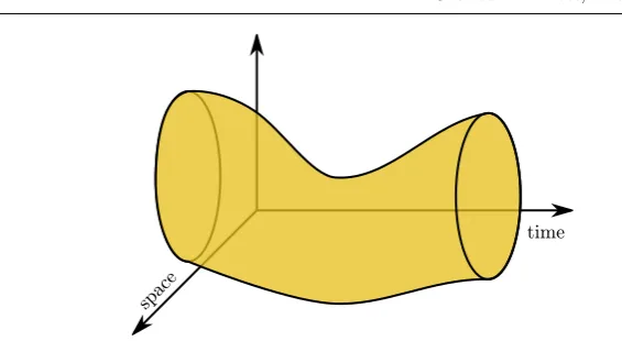
Fig. 2.1: A sketch of the space-time domainGT.
Ω(t). It follows thatΓ(t) admits a description as the zero level set of a signed distance functiond(·, t) :Rn+1 →Rso that d(·, t)<0 in Ω(t) and d(·, t)>0 in ¯Ω(t)c. We denote byG
T for the space-time domain given by
GT =
[
t∈[0,T]
Γ(t)× {t}. (2.1)
For our analysis, it is sufficient to considerd(·, t) locally toΓ(t). We restrict our considerations toN(t), an open neighbourhood ofΓ(t). We choose N(t) so that|∇d(x, t)| 6= 0 forx∈ N(t) and assume that
d, dt, dxi, dxixj ∈C 2(
NT) fori, j= 1, . . . , n+ 1;
here NT =St∈[0,T]N(t)× {t}. The orientation of Γ(t) is fixed by choosing
ν as the outward pointing normal, so thatν(x, t) =∇d(x, t). For (x, t)∈ GT, we denoteP =P(x, t) the projection operator onto the tangent spaceTxΓ(t), given by Pij(x, t) = δij−νi(x, t)νj(x, t) and by H=H(x, t) the (extended) Weingarten map (or shape operator),
Hij(x, t) = (νi(x, t))xj =dxixj(x, t).
We will use the fact thatPH=HP =H. Finally, we denote byH =H(x, t) the mean curvature ofΓ(t)
H(x, t) = traceH(x, t) = n+1
X
i=1
Hii(x, t).
For a functionη:Γ(t)→R, we define its tangential gradient∇Γη by
where ηe is a smooth extension of η away from Γ(t). It can be shown that this definition is independent of the choice of extension. We denote then+ 1 components of∇Γη by
∇Γη = (D1η, . . . , Dn+1η).
The Laplace-Beltrami operator is given by
∆Γη=∇Γ · ∇Γη = nX+1
j=1
DjDjη.
We will denote by dσ the surface measure on Γ(t) which admits the fol-lowing formula for partial integration for a portion M(t) ⊆Γ(t) [11, Theo-rem 2.10]: Z
M(t)∇
Γηdσ=
Z
M(t)
ηHνdσ+
Z
∂M(t)
ηµdσ, (2.2)
where µ is the co-normal to ∂M(t) which is normal to ∂M(t) but tangent to Γ(t). IfM(t) =Γ(t) and has no boundary, the boundary term vanishes. Furthermore, we have a Green’s formula onΓ(t) [11, Theorem 2.14]:
Z
Γ(t)∇
Γη· ∇Γϕdσ=−
Z
Γ(t)
ϕ∆Γηdσ. (2.3)
These formulae allow the definition of weak derivatives and Sobolev spaces. We define the spaceW1,q(Γ(t)) by
W1,q(Γ(t)) :=η∈Lq(Γ(t)) :Djη∈Lq(Γ(t)) forj= 1, . . . , n+ 1 ,
with norm
kηkW1,q(Γ(t))=
kηkqLq(Γ(t))+k∇ΓηkqLq(Γ(t)) 1
q
.
This can be easily extended to higher order spaces. See [11] for details. We will use the notationHk(Γ(t)) forWk,2(Γ(t)).
We will make use of the following Sobolev embeddings:
Lemma 2.1 ([25, Theorems 2.5 and 2.6])ForΓ(t) as above, we have
W1,q(Γ(t))
⊂
(
Lnq/(n−q)(Γ(t)) forq < n
C0(Γ(t)) forq > n. (2.4)
Furthermore there exists a constantc=c(n, q), independent oft, such that for any η∈W1,q(Γ(t)),
kηkLnq/(n−q)(Γ(t))≤ckηkW1,q(Γ(t)) forq < n (2.5a)
In particular, this allows us to embedH1(Γ(t)) inL6(Γ(t)) for all
dimen-sions (n= 1,2,3) so thatkψ′(η)k
L2(Γ(t)) ≤c kηk
3
H1(Γ(t))+kηkH1(Γ(t))
. Further, we assume that for each (x, t) ∈ NT there exists a unique p=
p(x, t)∈Γ(t), such that
x=p(x, t) +d(x, t)ν(p(x, t), t). (2.6)
See [23, Chapter 14] for a proof. We extendν, P andHto functions onNT by setting
ν(x, t) =ν(p(x, t), t) =∇d(x, t),
and similarly P(x, t) = P(p(x, t), t) = Id−ν(x, t)⊗ν(x, t) and H(x, t) =
∇2d(x, t) for (x, t)
∈ NT.
Although it is sufficient to describe the evolution of the surface through a normal velocity, we wish to consider material surfaces for which a material particle, atX(t) onΓ(t), has a material velocity ˙X(t) not necessarily only in the normal direction. The normal velocity of the surface can be calculated to bevν=−dtν. We sayvτis a tangential velocity field ifvτ·ν = 0 inNT. Given a tangential velocity fieldvτ, we call
v:=vτ+vν
a material velocity field. We assume that we are given a global velocity fieldv
so that pointsX(t) evolve with the velocity ˙X(t) =v(X(t), t). We will assume thatv∈C2(N
T).
2.2 Material derivative and transport formulae
Given a family of surfaces {Γ(t)} evolving in time with normal velocity field
vν, we define the normal time derivative∂◦ of a functionη:GT →Rby
∂◦η:= ∂eη
∂t +vν· ∇eη. (2.7)
Here,ηedenotes a smooth extension ofηtoNT. This derivative describes how a quantity η evolves in time with respect to the evolution of Γ(t). It can be shown that this definition is an intrinsic surface derivative, independent of the choice of extension.
Given a tangential vector field vτ, we define the material derivative of a scalar functionη:GT →R, by
∂•η:=∂◦η+vτ· ∇Γη=
∂eη
∂t +v· ∇eη.
Lemma 2.2 (Transport formula[12, Lemma 2.1])LetM(t)be an evolving surface with normal velocityvν. Letvτ be a tangential velocity field on M(t).
Let the boundary ∂M(t) evolve with velocity v =vν+vτ. Assume that η, ϕ
are functions such that all the following quantities exist. Then, we obtain the identity
d dt
Z
M(t)
ηdσ=
Z
M(t)
∂•η+η∇Γ ·vdσ. (2.8)
Furthermore, we have
d dt
Z
M(t)
ηϕdσ=
Z
M(t)
∂•η ϕ+η ∂•ϕ+ηϕ∇Γ ·vdσ. (2.9)
Let A=A(x, t)be a matrix which is positive definite on the tangent space to
Γ(t). Denote by D(v) the rate of deformation tensor given by
D(v)ij = 1 2
nX+1
k=1
AikDkvj+AjkDkvi fori, j= 1, . . . , n+ 1, (2.10)
and by B(v) the tensor
B(v) :=∂•A+∇Γ ·vA −2D(v). (2.11)
Then we have the formula
d dt
Z
M(t)A∇
Γη· ∇Γϕdσ=
Z
M(t)A∇
Γ∂•η· ∇Γϕ+A∇Γη· ∇Γ∂•ϕdσ
+
Z
M(t)B
(v)∇Γη· ∇Γϕdσ.
(2.12)
We conclude this subsection with a result allowing us to extend functions defined on one surface to the whole space-time domain.
Lemma 2.3 Fix t∈[0, T]and letη∈H1(Γ(t)), respectivelyC1(Γ(t)). Then there exists an extension ηe: GT → R such that ηe|t = η and eη ∈ H1(Γ(s)),
resp.C1(Γ(s)), for all timess
∈[0, T]and∂•ηe= 0.
Proof The ordinary differential equation:
d
dsX(s) =v(X(s), s) fors∈[0, T], X(t) =x,
determines a flowφs(x) onGT forx∈Γ(t) such that
φs(x)∈Γ(s) for alls∈[0, T] andφt(x) =x.
We define the extensionηeby
e
η(x, s) :=η((φs)−1(x)) for (x, s)∈ GT.
It is clear that since (φs)−1 ∈ C1(Γ(t);Γ(s)), we have ηe∈ H1(Γ(s)) (resp.
C1(Γ(s))) for all timess
∈[0, T].
Finally, we can calculate for y= (φs)−1(x),
∂•eη(x, s) = d
dsηe(φs(y), s) =
d
dsη(y) = 0 for (x, s)∈ GT,
which shows the result. ⊓⊔
2.3 Derivation of Cahn-Hilliard equations
We will consider a conservation law on an evolving surface with a diffusive flux driven by a chemical potential. This is the approach taken by [21]. In general, the Ginzburg-Landau functional onΓ(t) will not decrease along the trajectory of solutions.
Let urepresent a density of a scalar quantity on Γ(t). Following [12], we arrive at the pointwise conservation law
∂◦u+u∇Γ ·vν+∇Γ ·q= 0. (2.13)
Hereq represents the tangential flux ofuon{Γ(t)}.
We will assume that the flux q is the sum of a diffusive flux qd and an advective fluxqa:
qd =−∇Γw and qa=uvτ.
The diffusive flux is driven by the gradient of chemical potential w gives us the split system [16]
∂•u+u∇Γ ·v−∆Γw= 0 (2.14a)
−ε∆Γu+ 1
εψ
′(u)
−w= 0. (2.14b)
This leads to the fourth order Cahn-Hilliard equation onGT:
∂•u+u∇Γ ·v=∆Γ
−ε∆Γu+ 1
εψ
′(u). (2.15)
We close the system with the initial condition
u(·,0) =u0 onΓ0. (2.16)
There are no boundary conditions since the boundary ofΓ(t) is empty.
Remark 2.1 One can derive the Cahn-Hilliard equations posed in a Cartesian domain as anH−1gradient flow of the Ginzburg-Landau functional. To obtain
2.4 Solution spaces
In standard parabolic theory one looks for solutions in Bochner spaces. Con-sidering our Cahn-Hilliard equation on a Cartesian domainΩ[15], one would expect solutions to live in the spaces
u∈L∞(0, T;H1(Ω)), u′ ∈L2(0, T;H−1(Ω)), w∈L2(0, T;H1(Ω)).
These spaces are constructed by considering uas a function from (0, T) into the Hilbert spaceH1(Ω). We would like to extend this definition so that u(t)
is in the now time-dependent Hilbert space H1(Γ(t)). We consider Sobolev
spaces over the space-time domainGT. We will write ∇GT for the space-time
gradient and dσT for the space-time measure onGT. This approach is similar to the Eulerian formulation of [28]. We contrast our approach with that of [33], who proposed using an equivalent formulation using a reference domain.
We start by presenting the space-time domainsL2(
GT) andH1(GT) defined by
L2(GT) :=
η∈L1loc(GT) :
Z
GT
η2dσT <+∞
H1(GT) :=
n
η∈L2(GT) :∇GTη∈L 2(
GT)
o
.
with norms
kηkL2(GT):=
Z
GT
η2dσT
1 2
kηkH1(G
T):=
kηk2L2(G
T)+k∇GTηk 2
L2(G
T) 1
2
.
Proposition 2.1 ([25, Theorem 2.9])The spaceH1(G
T)is compactly
embed-ded into L2(G
T).
Using the identities,
Z T
0
Z
Γ(t)
ηdσdt=
Z
GT
η
q
1 +|vν|2 dσT,
and
∇GTη= ∇Γη+
∂◦η vν 1 +|vν|2
, ∂
◦η
1 +|vν|2
!
,
our assumptions on v imply that the space-time norms can be replaced with the equivalent norms
kηk′L2(G
T):= Z T
0
Z
Γ(t)
η2dσdt
!1 2
kηk′H1(G
T):= Z T
0
Z
Γ(t)
η2+|∇Γη|2+ (∂◦η)2dσdt
!1 2
We will use the equivalent primed norms (dropping the prime) onL2(
GT) and
H1(G
T) in the following. We define the spaceL2
L2 by
L2
L2 :=
(
η∈L1 loc(GT) :
Z T
0
Z
Γ(t)
ηdσdt <+∞
)
,
with the inner product
(η, ξ)L2
L2 := Z T
0
Z
Γ(t)
ηξdσdt.
It is clear thatL2
L2 is equivalent to L2(GT) and hence is a Hilbert space. Next, we define the spaceL2
H1 as
L2
H1 :=
η:GT →R:η∈L2L2 and∇Γη∈(L2L2)n+1 ,
with the inner product
(η, ξ)L2
H1 :=
Z T
0
Z
Γ(t)∇
Γη· ∇Γξ+ηξdσdt,
where ∇Γη should be interpreted in the weak sense. Notice that elements of this space are weakly differentiable at almost every time.
Lemma 2.4 The space L2
H1 is a Hilbert space.
Proof It is clear that L2
H1 is an inner product space and we are left to show completeness. Letηk be a Cauchy sequence inL2H1. This implies thatηk and
∇Γηk are Cauchy sequences in L2(GT) and (L2(GT))n+1. This means that there existsη ∈L2(G
T), ξ∈(L2(GT))n+1 such that
kηk−ηkL2(GT)+k∇Γηk−ξkL2(GT)→0 ask→ ∞.
Fixt∗ ∈(0, T) and letϕ∈C1(Γ(t∗)) andα∈C(0, T). UsingLemma 2.3, we
can construct ϕe: GT → R such that ϕe(·, t) =ϕ and ϕe ∈ C1(Γ(t)) for each timet∈(0, T). Then, forj = 1, . . . , n+ 1, we obtain
Z T
0
Z
Γ(t)
ηDj(αϕe) +ξj(αϕe) dσdt
=
Z T
0
Z
Γ(t)
(η−ηk)Dj(αϕe) + ηkDj(αϕe) +ξj(αϕe)dσdt
=
Z T
0
Z
Γ(t)
(η−ηk)Dj(αϕe) + (−Djηk+ξj)(αϕe) dσdt,
where we have used the fact that ηk is weakly differentiable at almost every time. Taking the limitk→ ∞, we infer
Z T
0
α
Z
Γ(t)
ηDjϕe+ξjϕedσ
!
Since this holds for allα∈C(0, T), by the Fundamental Lemma of the Calculus of Variations, att=t∗, we have
Z
Γ(t∗)
ηDjϕ+ξjϕdσ= 0 for allϕ∈C1(Γ(t∗)).
Since the choice oft∗ was arbitrary, we infer thatξis the weak gradient ofη
for almost every timet∈(0, T) and the proof is complete. ⊓⊔
The equivalence of norms implies that η ∈ L2
H1 with ∂•η ∈ L2L2 if, and only if,η∈H1(
GT).
For 1≤q≤ ∞, we will define the spaceLqH1 by
LqH1:=
n
η∈Lq(GT) :kηkLq
H1 <+∞
o
,
with norm
kηkLq H1 :=
Z T
0 k
ηkqH1(Γ(t)) dt
!1
q
forq <∞,
ess sup t∈(0,T)k
ηkH1(Γ(t)) forq=∞.
It is clear thatL∞H1 ⊂L2H1 and that
kηkL2
H1 ≤
√
TkηkL∞
H1 for allη∈L
∞
H1.
Finally, we defineL∞H2 andL2H2 by
L∞H2 :=
(
η∈L2(GT) : ess sup t∈(0,T)k
ηkH2(Γ(t))<+∞
)
L2H2 :=
(
η∈L2(GT) :
Z T
0 k
ηk2H2(Γ(t)) dt <+∞
)
.
Remark 2.2 As a restriction on our analysis we will only consider ∂•u as a
function in L2
L2 since we do not wish to consider a weak material derivative. Such considerations are left to future work.
We conclude this section with a result which will take an integral in time equality into an almost everywhere in time equality. The proof is the general-isation of a similar result given in [30, Lemma 7.4] for planar domains.
Lemma 2.5 Let η∈L2
H1 with
Z T
0
Z
Γ(t)∇
Γη· ∇Γξ+ηξdσdt= 0 for allξ∈L2H1. (2.17)
Then for almost all timest∈(0, T),
Z
Γ(t)∇
Proof Fixϕ∈L2
H1 andα∈C([0, T]), then choosingξ=αϕ∈L2H1 and
0 =
Z T
0
Z
Γ(t)∇
Γη· ∇Γξ+ηξdσdt=
Z T
0
α
Z
Γ(t)∇
Γη· ∇Γϕ+ηϕdσ
!
dt.
Since the choice ofαwas arbitrary, the Fundamental Lemma of the Calculus
of Variations implies the result. ⊓⊔
2.5 Weak and variational form
We start by multiplying (2.14a,2.14b) by a test functionϕand apply integra-tion by parts to the Laplacian terms to give the weak form. This will be the definition of solution used throughout this paper. Existence and uniqueness of solutions will be shownSection 4.
Definition 2.1 (Weak solution) We say that the pair (u, w) :GT → R2, withu∈L∞H1∩H1(GT) andw∈L2H1, are a weak solution of the Cahn-Hilliard equation (2.15) if, for almost every time t∈(0, T),
Z
Γ(t)
∂•uϕ+uϕ∇Γ ·v+∇Γw· ∇Γϕdσ= 0 (2.19a)
Z
Γ(t)
ε∇Γu· ∇Γϕ+ 1
εψ
′(u)ϕ
−wϕdσ= 0, (2.19b)
for allϕ∈L2
H1,
andu(·,0) =u0 pointwise almost everywhere inΓ0.
Restricting our thoughts to ϕ∈ H1(
GT), applying the transport formula to the first two terms in (2.19a) gives the variational formulation:
d dt
Z
Γ(t)
uϕdσ
!
+
Z
Γ(t)∇
Γw· ∇Γϕdσ=
Z
Γ(t)
u∂•ϕdσ (2.20a)
Z
Γ(t)
ε∇Γu· ∇Γϕ+ 1
εψ
′(u)ϕdσ=Z
Γ(t)
wϕdσ. (2.20b)
We remark that this formulation has no explicit mention of the velocity field
v and will be the basis of our finite element calculations.
It will be useful to write these equations using abstract bilinear forms. We define the following three to describe the above equations forη, ϕ∈H1(Γ(t)):
m(η, ϕ) =
Z
Γ(t)
ηϕdσ a(η, ϕ) =
Z
Γ(t)∇
Γη· ∇Γϕdσ
g(v;η, ϕ) =
Z
Γ(t)
This lets us write (2.19) as
m(∂•u, ϕ) +g(v;u, ϕ) +a(w, ϕ) = 0
εa(u, ϕ) +1
εm(ψ
′(u), ϕ)
−m(w, ϕ) = 0, (2.21)
and (2.20) as
d
dtm(u, ϕ) +a(w, ϕ) =m(u, ∂
•ϕ)
εa(u, ϕ) +1
εm(ψ
′(u), ϕ) =m(w, ϕ).
(2.22)
We may also write the results ofLemma 2.2in this form:
d
dtm(η, ϕ) =m(∂
•η, ϕ) +m(η, ∂•ϕ) +g(v;η, ϕ)
d
dta(η, ϕ) =a(∂
•η, ϕ) +a(η, ∂•ϕ) +b(v;η, ϕ),
with the addition of
b(v;η, ϕ) =
Z
Γ(t)B
(v)∇Γη· ∇Γϕdσ,
usingA= Id in the definition ofB(v).
3 Finite element approximation
In this section, we propose a finite element method for approximating solu-tions of the Cahn-Hilliard equation (2.15) based on the evolving surface finite element method [8].
3.1 Evolving triangulation and discrete material derivative
Let Γh,0 be a polyhedral approximation of the initial surface Γ0 with the
restriction that the nodes {X0
j}Nj=1 of Γh,0 lie on Γ0. We evolve the nodes
{Xj(t)}Nj=1 by the smooth surface velocity:
˙
Xj(t) =v(Xj(t), t), Xj(0) =Xj0, forj= 1, . . . , N.
Linearly interpolating between these nodes defines a family of discrete surfaces
{Γh(t)}. At each time, we assume that we have a triangulationTh(t) ofΓh(t), withhthe maximum diameter of elements inTh(t) uniformly in time:
h:= sup t∈(0,T)
max
E(t)∈Th(t)diamE(t). (3.1)
Remark 3.1 In practical situations, assuming a uniformly regular mesh may not be feasible. Large surface deformations can lead to poor quality triangu-lations with deformed elements. In such cases, re-meshing may be required [4,
14]. Alternatively, one may use an arbitrary Lagrangian-Eulerian formulation by allowing extra tangential mesh motions [19,20].
We define νh element-wise as the unit outward pointing normal to Γh(t) and denote by∇Γh the tangential gradient on Γh(t) defined element-wise by
∇Γhηh:=∇eηh−(∇eηh·νh)νh= (Id−νh⊗νh)∇ηeh=:Ph∇ηeh.
This is a vector-valued quantity and we will denote its components by
∇Γhηh= Dh,1ηh, . . . , Dh,n+1ηh
We define the finite element space of piecewise linear functions onΓh(t) by
Sh(t) :={φh∈C(Γh(t)) :φh|E(t) is affine linear, for eachE(t)∈Th(t)}. (3.2) We will write{φN
j (·, t)}Nj=1for the nodal basis ofSh(t) given byφNj (Xi(t), t) =
δij.
The definition of a basis of Sh(t) allows us to characterise the velocity of the surface{Γh(t)}. An arbitrary pointX(t) onΓh(t) evolves according to the discrete velocityVh given by
˙
X(t) =Vh(X(t), t) := N
X
j=1
˙
Xj(t)φNj (X(t), t) = N
X
j=1
v(Xj(t), t)φNj (X(t), t).
(3.3) We will write Gh,T as the discrete equivalent to GT:
Gh,T :=
[
t∈(0,T)
Γh(t)× {t}. (3.4)
The discrete velocity Vh induces a discrete material derivative. For a scalar quantityηh onGh,T, we define the discrete material derivative∂h•ηh by
∂h•ηh:=∂tηeh+∇ηeh·Vh, (3.5)
whereηeh is an arbitrary extension ofηhto NT. This leads to the remarkable transport property of the basis functions{φN
j }.
Lemma 3.1 (Transport of basis functions[8, Proposition 5.4])LetφN
j :Gh,T →
Rbe a nodal basis function as described above, then
∂h•φNj = 0. (3.6)
From a practical view point, a key advantage of this methodology is that, since basis functions have zero discrete material velocity, there is no mention of the velocity or curvature in the resulting finite element scheme.
Lemma 3.2 (Transport lemma for triangulated surfaces[12, Lemma 4.2]) Let {Γh(t)} be a discrete family of triangulated surfaces evolving with velocity
Vh. Letηh, φh be time-dependent finite element functions such that the
follow-ing quantities exist. Then, we have
d dt
Z
Γh(t)
ηhdσh=
Z
Γh(t)
∂h•ηh+ηh∇Γh·Vhdσh. (3.7)
In particular, for theL2 inner product this means that
d dt
Z
Γh(t)
ηhφhdσh=
Z
Γh(t)
(∂h•ηh)φh+ηh(∂h•φh) +ηhφh∇Γh·Vhdσh, (3.8)
and for the Dirichlet inner product, we obtain
d dt
Z
Γh(t)
∇Γhηh· ∇Γhφhdσh
=
Z
Γh(t)
∇Γh(∂
•
hηh)· ∇Γhφh+∇Γhηh· ∇Γh(∂
•
hφh) dσh
+ X
E(t)∈Th(t)
Z
E(t)B
h(Vh)∇Γhηh· ∇Γhφhdσh,
(3.9)
where
Bh(Vh) = 1
2(∇Γh·Vh)Id−Dh(Vh) and Dh(Vh)ij =
1
2 Dh,iVh,j+Dh,jVh,i
.
Lemma 3.3 Under our assumptions on {Γh(t)}, we have that
sup t∈[0,T]
k∇Γh·VhkL∞(Γ
h(t))+kBh(Vh)kL∞(Γ
h(t))
≤c sup
t∈[0,T]k
vkC2(NT).
(3.10)
Proof The result follows from applying the geometric estimates (3.23) and (3.42) along with our assumption thatv∈C2(
NT). ⊓⊔
3.2 Finite element scheme
We will assume that there exists a mesh sizeh0>0 such thatkU0kH1(Γ
h,0)is bounded independently of hfor h < h0. This implies that there exists C >0
such that for allh < h0, we have
Eh
0 :=
Z
Γh,0
ε
2|∇ΓhU0| 2
+1
εψ(U0) dσh< C. (3.11)
Remark 3.2 One particular choice of initial condition will be to takeU0 as a
suitable approximation of u0 (for example, Πhu0 defined in (3.45)) for u0 ∈
Our solution spaces will be
e
ShT :={φh∈C(Gh,T) :φh(·, t)∈Sh(t) for allt∈[0, T]}
ShT :={φh∈SehT :∂h•φh∈C(Gh,T)}.
(3.12)
The finite element scheme is: Given U0, find Uh∈ShT andWh ∈SehT such that for almost every timet∈(0, T)
d dt
Z
Γh(t)
Uhφhdσh
!
+
Z
Γh(t)
∇ΓhWh· ∇Γhφhdσh= Z
Γh(t)
Uh∂h•φhdσh
(3.13a)
Z
Γh(t)
ε∇ΓhUh· ∇Γhφh+
1
εψ
′(U
h)φhdσh=
Z
Γh(t)
Whφhdσh
(3.13b)
for allφh∈Sh(t),
subject to the initial condition
Uh(·,0) =U0. (3.14)
The transport formula (3.8) implies that, forφh∈ShT, (3.13a) is equivalent to
Z
Γh(t)
∂h•Uhφh+Uhφh∇Γh·Vh+∇ΓhWh· ∇Γhφhdσh= 0. (3.15)
We can write these equations in matrix form. First, we will introduce vec-torsα(t), β(t)∈RN for the nodal values ofUh andWh by
Uh(x, t) = N
X
j=1
αj(t)φNj (x, t), Wh(x, t) = N
X
j=1
βj(t)φNj (x, t) for (x, t)∈ Gh,T.
In place of the bilinear forms, we have the mass matrix M(t) and stiffness matrixS(t):
M(t)ij =
Z
Γh(t)
φNi φNj dσh S(t)ij=
Z
Γh(t)
∇Γhφ
N i · ∇Γhφ
N j dσh,
and in place of the non-linear term, we will write
F(α(t))j=
Z
Γh(t)
ψ′
N
X
i=1
αi(t)φNi
!
φNj dσh.
Using the transport of basis property (Lemma 3.1), we can write (3.13) as
d
dt(M(t)α(t)) +S(t)β(t) = 0 (3.16a)
εS(t)α(t) +1
Alternatively, eliminatingβ(t), this can be written as
d
dt(M(t)α(t)) +S(t)M(t)
−1
εS(t)α(t) +1
εF(α(t))
= 0. (3.17)
One could also use lumped mass integration [32, Chapter 15] instead of the full mass matrix.
Notice that this is the same structure as a finite element discretisation of a Cahn-Hilliard equation posed on a planar domain. We now have time de-pendent matrices which need to be assembled on each time step. Various time stepping schemes have been considered for second-order parabolic problems on evolving surfaces [10,13,26].
Next, we introduce abstract notation which permit a more compact writing of the analysis that follows:
mh(ηh, φh) =
Z
Γh(t)
ηhφhdσh ah(ηh, φh) =
Z
Γh(t)
∇Γhηh· ∇Γhφhdσh
gh(Vh;ηh, φh) =
Z
Γh(t)
ηhφh∇Γh·Vhdσh.
This lets us write (3.13) as
d
dtmh(Uh, φh) +ah(Wh, φh) =mh(Uh, ∂
•
hφh)
εah(Uh, φh) + 1
εmh(ψ
′(U
h), φh) =mh(Wh, φh),
and (3.15) as
mh(∂h•Uh, φh) +gh(Vh;Uh, φh) +ah(Wh, φh) = 0.
The transport laws fromLemma 3.2 transfer to the abstract setting also:
d
dtmh(ηh, φh) =mh(∂
•
hηh, φh) +mh(ηh, ∂h•φh) +gh(Vh;ηh, φh) d
dtah(ηh, φh) =ah(∂
•
hηh, φh) +ah(ηh, ∂•hφh) +bh(Vh;ηh, φh),
where
bh(Vh;ηh, φh) =
X
E(t)∈Th(t)
Z
E(t)B
h(Vh)∇Γhηh· ∇Γhφhdσh.
Under the above assumptions, the following estimates are possible.
Theorem 3.1 (Well-posedness of the finite element scheme (3.13)) Under the above assumptions onU0and{Γh(t)}, there exists a unique solution
pair (Uh, Wh) ∈ ShT ×SehT, both with C1 in time nodal values, to the finite
element scheme (3.13)andRΓh(t)Uhdσh is conserved:
Z
Γh(t)
Uhdσh=
Z
Γh,0
Furthermore, there exists h1, 0< h1< h0, andC0 >0, which depend on the final time T and theH1(Γ
h,0)-norm of the initial condition U0, such that for allh < h1 the following bound is satisfied:
sup t∈(0,T)
Z
Γh(t)
ε
2|∇ΓhUh| 2
+1
εψ(Uh) dσh+
1 2
Z T
0 k∇
ΓhWhk 2
L2(Γ
h(t)) dt≤C0.
(3.19)
The proof will be shown after we have proven some intermediate results.
3.3 Lifted finite elements
The following analysis will rely on lift operators defined using a time dependent closest point operatorp(2.6). This lifting process will also be applied to the surface triangulation. This will induce a further discrete material velocityvh which will describe how the lifts of triangles on{Γ(t)}evolve.
First, for a functionηh: Gh,T →R, we define its lift,ηℓh:GT →R, implicitly, by:
ηℓ
h(p(x, t), t) =ηh(x, t), (3.20)
and, for a functionη:GT →R, we define its inverse lift,η−ℓ:Gh,T →Rby
η−ℓ(x, t) :=η(p(x, t), t). (3.21)
It is clear that these operations are inverses of each other
(η−ℓ)ℓ=η and (ηℓ
h)−ℓ=ηh.
Furthermore, (2.6) allows us to define a lifted triangulationTℓ
h(t) ofΓ(t) by
Thℓ={e(t) =Eℓ(t) :E(t)∈Th(t)}, Eℓ(t) :={p(x, t) :x∈E(t)}. (3.22) This defines an exact triangulation ofΓ(t).
Lemma 3.4 (Stability of lift [8, for q = 2]) Let ηh: Gh,T → R, with lift
ηhℓ:GT → R, be such that the following quantities exist. For 1 ≤ q ≤ +∞,
there exists c1, c2 > 0, independent of h, but depending on q, such that for each time t ∈ [0, T] and each element E(t) ∈ Th(t) with associated lifted
elemente(t)∈Tℓ
h(t), the following hold:
c1
ηhℓ
Lq(e(t))≤ kηhkLq(E(t)) ≤c2
ηℓh
Lq(e(t)) (3.23a)
c1
∇Γηhℓ
Lq(e(t))≤ k∇ΓhηhkLq(E(t))≤c2
∇Γηhℓ
Lq(e(t)) (3.23b)
∇2
Γhηh
L2(E(t))≤c
∇2Γηℓh
L2(e(t))+h
∇Γηhℓ
L2(e(t))
. (3.23c)
Lemma 3.5 ForΓh(t) as above,
W1,q(Γh(t))⊂
(
Lnq/(n−q)(Γ
h(t)) forq < n
L∞(Γh(t)) forq > n.
(3.24)
Furthermore there exists a constant c =c(n, q), independent of h, such that for any ηh∈W1,q(Γh(t))
kηhkLnq/(n−q)(Γ
h(t))≤ckηhkW1,q(Γh(t)) forq < n (3.25a)
kηhkL∞(Γ
h(t))≤ckηhkW1,q(Γh(t)) forq > n. (3.25b)
Proof To see the embedding result, we apply Lemma 2.1. The bounds then follow using the stability of the lift (Lemma 3.4). ⊓⊔
We will write Sℓ
h(t) for the space of lifted finite element functions:
Sℓh(t) ={ϕh=φhℓ :φh∈Sh(t)}.
This space comes with the standard approximation property:
Proposition 3.1 (Approximation property) The Lagrangian interpola-tion operator Ih: C(Γ(t)) → Shℓ(t) is well defined and, for z ∈ H2(Γ(t)),
satisfies the bound
kz−IhzkL2(Γ(t))+hk∇Γ(z−Ihz)kL2(Γ(t)) ≤ch2kzkH2(Γ(t)). (3.26)
Let 1≤q≤ ∞be such thatH1(Γ(t))embeds intoLq(Γ(t)), then
k∇Γ(z−Ihz)kLq(Γ(t))≤ch1+min(0,n/q−n/2)kzkH2(Γ(t)). (3.27)
Proof The proof is given in [7] for the case q= 2 and can be easily extended using standard interpolation theory [3, Theorem 3.1.6] to the caseq6= 2. ⊓⊔
Remark 3.3 For the remainder of the paper, we will write lower case letters for the lift finite element functions with capital letters (i.e.Uℓ
h=uhandWhℓ=wh) andϕh for the lift ofφh.
The motion of the edges of the simplices in the triangulation {Tℓ h(t)} defines a discrete material velocity for the surface {Γ(t)}. Let X(t) be the trajectory of a point on {Γh(t)} with velocity Vh(X(t), t). We set Y(t) =
p(X(t), t) then definevh by
vh(Y(t), t) := ˙Y(t) =
∂p
∂t(X(t), t) +∇p(X(t), t)·Vh(X(t), t), (3.28)
so that forx∈Γh(t), using (2.6), we have
This defines another discrete material derivative for functionsϕh(·, t)∈Shℓ(t). We define the discrete material derivative onGT element-wise by
∂h•ϕh:=∂tϕh+vh· ∇ϕh. (3.29)
A quick calculation [12] shows that for allφh∈Sh(t), with liftϕh∈Shℓ(t),
∂h•ϕh= (∂h•φh)ℓ. (3.30)
It can be shown, similarly to (3.6), that ∂•
h(φNj )ℓ= 0. We will writeS ℓ,T
h and
e
Shℓ,T for the lifts of the spaces ST
h and SehT defined by (3.12). It is clear that fromLemma 3.4 that
Shℓ,T ⊂H1(GT) and Sehℓ,T ⊂L
2
H1.
We remark that the continuous and discrete material velocities on {Γ(t)} only differ in the tangential direction. This implies that the difference between the two material derivatives on{Γ(t)}only depends on the tangential gradient of the original function and not on any time derivatives.
These definitions also permit transport formulae:
Lemma 3.6 (Transport lemma for smooth triangulated surfaces [12, Lemma 4.2])Let{Γ(t)}be an evolving surface decomposed at each time into a family curved elements{Tℓ
h(t)}whose edges evolve with velocityvh. Then the
following relations hold for functions ηh, ϕh:GT →R such that the following
quantities exist:
d dt
Z
Γ(t)
ηhdσ=
Z
Γ(t)
∂h•ηh+ηh∇Γ ·vhdσ, (3.31)
and
d
dtm(ηh, ϕh) =m(∂
•
hηh, ϕh) +m(ηh, ∂h•ϕh) +g(vh;ηh, ϕh) (3.32) d
dta(ηh, ϕh) =a(∂
•
hηh, ϕh) +a(ηh, ∂h•ϕh) +b(vh;ηh, ϕh). (3.33)
3.4 Proof of finite element scheme well-posedness
Before showing stability of the finite element scheme, we will show a generalised Gronwall inequality:
Lemma 3.7 Let yh(t), zh(t)≥0and satisfy the following differential
inequal-ity forCe≥0
d
dtyh(t) +zh(t)≤c yh(t) +hyh(t)
2+h2y
h(t)3+Ce
for0≤t≤T,
yh(0) =y0.
Lethbe sufficiently small so that1−h(y0+Ce)2(e2(1+h)ct−1)>0, thenyh, zh
satisfy the bound
yh(t) +
Z t
0
zh(s) ds≤
e(1+h)ct(y
0+Ce)
q
1−h(y0+Ce)2(e2(1+h)ct−1)
. (3.35)
Proof Let ηh(t) = yh(t) +R t
0zh(s) ds+Ce and η0 = y0+Ce. We note that
yh(t)q ≤ηh(t)q (q= 1,2,3) andηh(t)≥0. Thenηh satisfies
d
dtηh(t)≤c ηh(t) +hηh(t)
2+h2η
h(t)3≤c (1 +h)ηh(t) + (h+h2)ηh(t)3.
This implies
1 2 + 2h
d dtlog
η
h(t)2 1 +hηh(t)2
=
d dtηh(t)
(1 +h)ηh(t) + (h+h2)ηh(t)3 ≤c.
Assuming thathis sufficiently small so that 1−hη2
0(e2(1+h)ct−1)>0,
inte-grating this inequality in time implies
ηh(t)2≤ e
2(1+h)ctη2 0
1−hη2
0(e2(1+h)ct−1)
.
Rearranging this inequality gives the desired result. ⊓⊔
We can now show the stability result in Theorem 3.1.
Proof (Proof of Theorem3.1) Considering (3.17), since M(t) is positive def-inite, S(t) positive semi-definite and F is locally Lipschitz, standard the-ory of ordinary differential equations gives a unique short-time solution α∈ C1([0, T
0];RN) for someT0 < T. From (3.7), we know S(t) andM(t) areC1
in time, andM(t)−1∈C1by the Inverse Function Theorem. Thus, we infer
β(t) =M(t)−1S(t)M(t)−1(εS(t)α(t) +1
εF(α(t)))∈C
1([0, T 0];RN).
This is easily translated into solutionsUh, Wh in the appropriate spaces. Since φh = 1 is an admissible test function in (3.13a), it is clear that
R
Γh(t)Uhdσhis conserved.
To extend to the long-term solution, we construct an energy bound. We start by testing (3.13a) withWhand (3.13b) with∂h•Uh and sum to see
εah(Uh, ∂h•Uh) +1
εmh(ψ
′(U
h), ∂h•Uh) +ah(Wh, Wh)
Applying the transport formulae fromLemma 3.2, we obtain
d dt
εah(Uh, Uh) + 1
εmh(ψ(Uh),1)
+ah(Wh, Wh)
= ε
2bh(Vh;Uh, Uh) + 1
εgh(Vh;ψ(Uh),1)−gh(Vh;Uh, Wh).
Next, we introduce the L2(Γ
h(t)) projectionΛh: L2(Γh(t)) →Sh(t). For
z∈L2(Γ
h(t)), we defineΛhzas the unique solution of
mh(Λhz, φh) =mh(z, φh) for allφh∈Sh(t). (3.36)
Forz∈H1(Γ
h(t)), we will make use of the following bounds:
kΛhzkH1(Γh(t))≤ckzkH1(Γh(t)), kz−ΛhzkL2(Γh(t))≤chkzkH1(Γh(t)). (3.37) These bounds follow since our triangulation is quasi-uniform.
We first note that from our assumptions on v, we have Uh(∇Γ ·v)−ℓ ∈
H1(Γ
h(t)) with
Uh(∇Γ ·v)−ℓ
H1(Γ
h(t))≤ckUhkH1(Γh(t)). Next, we test (3.13b)
withΛh(Uh(∇Γ·v)−ℓ) and using (3.37) and the Sobolev embedding (Lemma3.5), we see that
Z
Γh(t)
WhΛh Uh(∇Γ ·v)−ℓdσh
≤εah(Uh, Λh Uh(∇Γ·v)−ℓ)
+1
ε
mh(ψ′(Uh), Uh(∇Γ ·v)ℓ)
+1
ε
mh(ψ′(Uh), Λh Uh(∇Γ ·v)−ℓ−Uh(∇Γ ·v)ℓ)
≤c
εah(Uh, Uh) +1
εmh(ψ(Uh),1)
+ch
ε kUhk
4
H1(Γh(t)).
Similarly, testing (3.13b) withWh leads to
mh(Wh, Wh)≤cεah(Uh, Uh) + 1
2ah(Wh, Wh) +
c ε2kUhk
6
H1(Γ
h(t)).
Applying the geometric bound (3.42), the two previous bounds, a Poincar´e inequality and the fact that the mass ofUhis conserved, we infer that
|g(Vh;Uh, Wh)|
≤mh(Wh, Uh ∇Γh·Vh−(∇Γ·v)
−ℓ)+m
h Wh, Λh(Uh(∇Γ ·v)−ℓ)
≤cmh(Uh, Uh) +ch2mh(Wh, Wh) +
mh Wh, Λh(Uh(∇Γ ·v)−ℓ)
≤c
εah(Uh, Uh) +1
εmh(ψ(Uh),1)
+1
whereCe0(U0) is a constant which only depends on the integral ofU0 onΓh,0.
This leads to the estimate d
dt
εah(Uh, Uh) +1
εmh(ψ(Uh),1)
+ah(Wh, Wh)
≤cε
εah(Uh, Uh) + 1
εmh(ψ(Uh),1) +h ah(Uh, Uh)
2+h2a
h(Uh, Uh)3
+Ce0(U0).
We will use the generalised Gronwall inequality from (3.35) with yh =
εah(Uh, Uh) + 1εmh(ψ(Uh),1), zh = ah(Wh, Wh) and Ce = Ce0(U0). Given T,
there existsh1, 0< h1< h0, such that forh < h1, we have
1−h(E0h+Ce0(U0))2(e2(1+h)ct−1)>0.
This gives the energy bound in (3.19) withC0given by
C0:=
e(1+h)cT(
Eh
0 +Ce0(U0))
q
1−h(Eh
0 +Ce0(U0))2(e2(1+h)ct−1)
This implies, that if h < h1, we have an energy bound on (0, T) and hence
can turn the short-time existence result in to existence over (0, T) whereT is
arbitrary. ⊓⊔
3.5 Geometric estimates
In this section, we will simply state the following geometric estimates without proof. Details can be found in [12, Section 5] except for (3.39c) and (3.39d) which can be found in [29, Lemma 3.3.14].
Lemma 3.8 Let µh denote the quotient of surface measuresdσ on Γ(t)and dσh onΓh(t) such thatµhdσh= dσ; then
sup t∈[0,T]
sup Γh(t)
|1−µh| ≤ch2 (3.38a)
sup t∈[0,T]k
∂h•µhkL∞(Γ
h(t))≤ch
2. (3.38b)
Lemma 3.9 Let Zh, φh ∈Sh(t)with lifts zh, ϕh∈Shℓ(t). Then the following
estimates hold for the given bilinear forms:
|mh(Zh, φh)−m(zh, ϕh)| ≤ch2kZhkL2(Γh(t))kφhkL2(Γh(t)) (3.39a)
|ah(Zh, φh)−a(zh, ϕh)| ≤ch2k∇ΓhZhkL2(Γ
h(t))k∇ΓhφhkL2(Γh(t))
(3.39b)
|gh(Vh;Zh, φh)−g(vh;zh, ϕh)| ≤ch2kZhkL2(Γ
h(t))kφhkL2(Γh(t)) (3.39c)
|bh(Vh;Zh, φh)−b(vh;zh, ϕh)| ≤ch2k∇ΓhZhkL2(Γ
h(t))k∇ΓhφhkL2(Γ
h(t)).
Using the same reasoning, it is also clear that
|mh(ψ′(Zh), φh)−m(ψ′(zh), ϕh)| ≤ch2kψ′(Zh)kL2(Γh(t))kφhkL2(Γh(t)). (3.40) Similar results apply if the first argument is the material derivative of a finite element function:
Lemma 3.10 ForZh ∈ShT, φh ∈SehT with liftszh, ϕh ∈Shℓ(t) for each time,
we have
|mh(∂•hZh, ϕh)−m(∂h•zh, φh)| ≤ch2k∂h•ZhkL2(Γh(t))kφhkL2(Γh(t)) (3.41a)
|ah(∂h•Zh, ϕh)−a(∂h•zh, φh)| ≤ch2k∇Γh(∂
•
hZh)kL2(Γ
h(t))k∇ΓhφhkL2(Γh(t)).
(3.41b)
The next lemma bounds errors from the approximation ofv byvh:
Lemma 3.11 The difference between the continuous velocity v and the dis-crete velocityvh on Γ(t)can be estimated by
|v−vh|+h|∇Γ(v−vh)| ≤ch2kvkC2(N
T)< ch
2. (3.42)
This allows us to bound the error between the material derivatives onΓ(t):
Corollary 3.1 Suppose that η: GT → R and ∂•η and ∂h•η exist. For η ∈
H1(Γ(t)), we have the estimate
k∂•η−∂h•ηkL2(Γ(t))≤ch2k∇ΓηkL2(Γ(t)), (3.43)
and forη∈H2(Γ(t)), we obtain
k∇Γ(∂•η−∂h•η)kL2(Γ(t))≤ch2kηkH2(Γ(t)). (3.44)
3.6 Ritz projection
We conclude this section by constructing a discrete projection operator, similar to an interpolation operator. We define the Ritz projection operator, Πhz ∈
Sh(t), ofz∈H1(Γ(t)) as the unique solution of
ah(Πhz, φh) =a(z, ϕh) for allφh∈Sh(t), with liftϕh∈Shℓ(t) (3.45)
and Z
Γh(t)
Πhzdσh=
Z
Γ(t)
zdσ.
Remark 3.4 This operator is the Ritz projection used by [6], but different to that used in other surface finite element analyses such as [9,12], which use the operatorRh:H2(Γ(t))→Shℓ(t) given as the unique solution of
a(Rhz, ϕh) =a(z, ϕh) for allϕh∈Shℓ(t) and
Z
Γ(t)R
hzdσ= 0.
The following bounds are immediate:
Theorem 3.2 Forz∈H1(Γ(t)),
kπhzkH1(Γ(t))≤ckzkH1(Γ(t)), kπhz−zkL2(Γ(t))≤chkzkH1(Γ(t)). (3.46)
Forz∈H2(Γ(t)),
kπhz−zkL2(Γ(t))+hk∇Γ(πhz−z)kL2(Γ(t)) ≤ch2kzkH2(Γ(t)), (3.47)
and for1≤q≤ ∞, such that H1(Γ(t))embeds into Lq(Γ(t)),
k∇Γ(πhz−z)kLq(Γ(t))≤ch1+min(0,n/q−n/2)kzkH2(Γ(t)). (3.48)
Proof TheH1stability result is clear and theL2error bound for aH1function
follows from an Aubin-Nitsche trick. The L2 results for z
∈H2(Γ(t)) follow
from standard error estimates for the surface finite element [7]. TheLq result follows from the same splitting argument along with an inverse inequality. ⊓⊔
Corollary 3.2 The Ritz projection is bounded in L∞ and we have the bound
kΠhzkL∞(Γ
h(t))≤ kπhzkL∞(Γh(t))≤ckzkH2(Γ(t)). (3.49)
Proof Let 1< q <∞be such that H1(Γ(t)) embeds into Lq(Γ(t)) and such that W1,q(Γ(t)) embeds into L∞(Γ(t)). The previous result, a Poincar´e
in-equality and (3.38a) imply that
kπhz−zkW1,q(Γ(t))≤ck∇Γ(πhz−z)kLq(Γ(t))+ Z
Γ(t)
πhz−zdσ
≤ckzkH2(Γ(t)),
forhsufficiently small. We use a Sobolev embedding (Lemma 2.1), to see
kπhzkL∞(Γ(t)) ≤ckπhzkW1,q(Γ(t))≤ckzkH2(Γ(t)).
It is clear that
kΠhzkL∞(Γ
h(t))=kπhzkL∞(Γ(t)),
Since ∂•
hΠhz6=Πh∂h•z, we also wish to have a bound on the discrete ma-terial derivative of this error for a function. We will assume thatz∈H2(Γ(t))
and ∂•z ∈H2(Γ(t)) for eacht. Under this assumption, we may take a time
derivative of (3.45), so that for allφh∈ShT with liftϕh∈Shℓ,T,
ah(∂•hΠhz, φh) =a(∂h•z, ϕh) + b(vh;z, ϕh)−bh(Vh;Πhz, φh). (3.50)
In fact using similar arguments to Lemma 2.3, we can construct a similar extension of a finite element functionφh∈Sh(t) to a functionφeh∈STh by
e
φh(x, s) = N
X
j=1
γjφNj (x, s) for (x, s)∈ Gh,T where φh(x) = N
X
j=1
γjφNj (x, t).
Hence, we deduce that (3.50) applies at each timet∈(0, T) forφh∈Sh(t). We start by proving two technical lemmas:
Lemma 3.12 Given z: GT →Rwith z ∈H2(Γ(t)) and∂•z ∈H2(Γ(t)) for
almost every timet∈(0, T), then ∂•hΠhz exists and we have the bound
∇Γh ∂
•
hΠhzL2(Γ
h(t))≤c kzkH2(Γ(t))+k∂
•zk
H2(Γ(t))
. (3.51)
Proof To show the bound, we start from (3.50), using a Young’s inequality, (3.47) and (3.39d) gives
ah(∂h•Πhz, φh)≤c k∇Γ∂•zk2L2(Γ(t))+kzk
2
H2(Γ(t))
+1
2k∇Γhφhk 2
L2(Γ
h(t)).
Applying this bound withφh=∂•hΠhz gives the estimate (3.51). ⊓⊔
Lemma 3.13 Define the function Th onShℓ(t)by
Th(ϕh) :=a(∂•h(πhz−z), ϕh). (3.52)
Then we have the bound
|Th(ϕh)| ≤ch
kzkH2(Γ(t))+k∂•zkH2(Γ(t))
k∇ΓϕhkL2(Γ(t)). (3.53)
Furthermore, for anyη ∈H2(Γ(t)), we have that
|Th(ϕh)| ≤chkzkH2(Γ(t))k∇Γ(ϕh−η)kL2(Γ(t))+ch2kzkH2(Γ(t))kηkH2(Γ(t))
+ch2kzkH2(Γ(t))+k∂•zkH2(Γ(t))
k∇ΓϕhkL2(Γ(t)).
(3.54)
Proof Using (3.45) and (3.50), we see forφh∈Sh(t), with liftϕh∈Shℓ(t),
Th(ϕh) =a(∂h•πhz, ϕh)−a(∂h•z, ϕh)
=b(vh;z−πhz, ϕh) + a(∂h•πhz, ϕh)−ah(∂•hΠhz, φh) + b(vh;πhz, ϕh)−bh(Vh;Πhz, φh)
Using our bound on the Ritz projection (3.47), and two geometric estimates (3.39d) and (3.41b), we have that
|Th(ϕh)| ≤chkzkH2(Γ(t))k∇ΓϕhkL2(Γ(t))
+ch2 k∇Γ∂•hπhzkL2(Γ(t))+k∇ΓπhzkL2(Γ(t))
k∇ΓϕhkL2(Γ(t))
≤chkzkH2(Γ(t))+k∂•zkH2(Γ(t))
k∇ΓϕhkL2(Γ(t)).
We can improve this estimate by comparing vh to the smooth velocityv and introducing a smooth functionη∈H2(Γ(t)). Then, we split the first term
inTh(ϕh) into
b(vh;πhz−z, ϕh)
=b(vh−v;πhz−z, ϕh) +b(v;πhz−z, ϕh−η) +b(v;πhz−z, η).
Using the smoothness of η, the final term, b(v;πhz−z, η), is bounded using an integration by parts argument given by [12, p. 21]:
b(v;ϕ, η) =
Z
Γ(t)
n+1
X
i,j=1
HνjB(v)ijϕ Diηdσ−
Z
Γ(t)
ϕ
nX+1
i,j=1
Dj B(v)ijDiη
dσ.
Hence, we obtain
|b(v;ϕ, η)| ≤ckϕkL2(Γ(t))kηkH2(Γ(t)).
Combining these calculations with (3.42) and (3.47), we get
|b(vh;πhz−z, ϕh)| ≤chkzkH2(Γ(t))k∇Γ(ϕh−η)kL2(Γ(t))
+ch2kzkH2(Γ(t)) k∇ΓϕhkL2(Γ(t))+kηkH2(Γ(t))
.
Hence, we have
|Th(ϕh)| ≤chkzkH2(Γ(t)k∇Γ(ϕh−η)kL2(Γ(t))+ch2kzkH2(Γ(t))kηkH2(Γ(t))
+ch2kzkH2(Γ(t))+k∂•zkH2(Γ(t))
k∇ΓϕhkL2(Γ(t)),
which is the second estimate. ⊓⊔
These results allow us to show an estimate for the difference between the material derivative of a function and its Ritz projection.
Lemma 3.14 Forz:GT →Rwithz, ∂•z∈H2(Γ(t)), we have
k∂h•(πhz−z)kL2(Γ(t))+hk∇Γ∂h•(πhz−z)kL2(Γ(t))
≤ch2 kzkH2(Γ(t))+k∂•zkH2(Γ(t))
Proof We start by rewriting the error as
a(∂h•(πhz−z), ∂•h(πhz−z))
=a(∂h•(πhz−z), ∂h•πhz−Ih(∂•z)) +a(∂h•(πhz−z), Ih(∂•z)−∂•z) +a(∂h•(πhz−z), ∂•z−∂h•z).
(3.56) We can bound the first term on the right-hand side using (3.53) by
|a(∂h•(πhz−z), ∂h•πhz−Ih(∂•z))|=|Th(∂h•πhz−Ih(∂•z))|
≤ch k∂•zkH2(Γ(t))+kzkH2(Γ(t))
k∇Γ(∂h•πhz−Ih(∂•z))kL2(Γ(t))
≤ch k∂•zkH2(Γ(t))+kzkH2(Γ(t))
k∇Γ∂h•(πhz−z)kL2(Γ(t)) +chk∇Γ∂h•(πhz−z)k2L2(Γ(t)).
The second term is bounded using the approximation property (3.26):
|a(∂h•(πhz−z), Ih(∂•z)−∂•z)| ≤chk∇Γ∂h•(πhz−z)kL2(Γ(t))k∂•zkH2(Γ(t)).
Finally, we use our estimate of the difference of material derivatives (3.43) to bound the third term:
|a(∂h•(πhz−z), ∂•z−∂h•z)| ≤ch2k∇Γ∂h•(πhz−z)kL2(Γ(t))kzkH2(Γ(t)).
Combining these three bounds in (3.56), we get the desired gradient norm bound forhsufficiently small.
To show theL2bound, we use the Aubin-Nitsche trick. We start by writing
e=∂•
h(πhz−z), theneis in L2 so can be set as the right-hand side for the dual problem: Findζ∈H1(Γ(t)) such that
a(ϕ, ζ) =m(e−c0, ϕ) for allϕ∈H1(Γ(t)), and
Z
Γ(t)
ζdσ= 0, (3.57)
wherec0= |Γ1(t)| R
Γ(t)edσ. We know [1] that (3.57) has a unique solution and
satisfies the regularity result
kζkH2(Γ(t)) ≤ckekL2(Γ(t)). (3.58)
We note that fromRΓ
h(t)Πhzdσh= R
Γ(t)zdσ, that
|Γ(t)| |c0|=
Z
Γ(t)
∂h•(πhz−z) dσ
= d dt
Z
Γ(t)
πhz−zdσ−
Z
Γ(t)
(πhz−z)∇Γ ·vhdσ.
We remark that from (3.38a) and (3.38b), we have
d dt
Z
Γ(t)
πhz−zdσ= d dt
Z
Γ(t)
πhz
1− 1
µh
dσ
!
≤ch2 kzkH2(Γ(t))+k∂•zkH2(Γ(t))
and using (3.47), we infer
Z
Γ(t)
(πhz−z)∇Γ ·vhdσ≤ckπhz−zkL2(Γ(t))≤ch2kzkH2(Γ(t)).
This implies
|c0| ≤ch2 kzkH2(Γ(t))+k∂•zkH2(Γ(t))
.
These calculations lead to
m(e, e)− |Γ(t)|2c2
0=a(ζ, e) =a(ζ−Ihζ, e) +Th(Ihζ). (3.59)
The first term on the right-hand side is bounded using the approximation property (3.26) and the gradient norm bound on e, together with the dual regularity result (3.58):
|a(ζ−Ih, e)| ≤ch2kekL2(Γ(t)) kzkH2(Γ(t))+k∂•zkH2(Γ(t))
.
The second term is estimated using the improved bound (3.54) on Th(Ihζ) withη=ζ. Applying the approximation (3.26) we see
|Th(Ihζ)| ≤ch2 kzkH2(Γ(t))+k∂•zkH2(Γ(t))
kekL2(Γ(t)).
Applying these two bounds in (3.59) gives the desired result. ⊓⊔
4 Well-posedness of the continuous problem
We use this section to show some properties of the continuous scheme based on the energy estimates coming from Theorem 3.1 along with further some estimates. We will use these properties in later sections but they are also important results in their own right.
4.1 Improved bounds on the finite element scheme
In order to derive some improved bounds on ∂h•Uh and Wh, we will assume that Uh,0 = Πhu0 with u0 ∈H2(Γ0). It is clear that assumption (3.11) still
holds in this case. In fact, we will make use of the bound
Eh
0 +Ce0(U0)≤cε 1 +ku0k2H2(Γ0)+ku0k4H2(Γ0)
+Cee1(u0) =:Ce1(u0), (4.1)
where
ee
C1(u0) :=cε
Z
Γ0
u0dσ
+
Z
Γ0
u0dσ
2
+
Z
Γ0
u0dσ
3!