Bayesian Sensitivity Analysis of a Cardiac Cell Model Using a Gaussian Process Emulator.

White Rose Research Online

Universities of Leeds, Sheffield and York

http://eprints.whiterose.ac.uk/

This is a copy of the final published version of a paper published via gold open access

in

PLoS One

This open access article is distributed under the terms of the Creative Commons

Attribution Licence (http://creativecommons.org/licenses/by/3.0), which permits

unrestricted use, distribution, and reproduction in any medium, provided the

original work is properly cited.

White Rose Research Online URL for this paper:

http://eprints.whiterose.ac.uk/87842

Published paper

Chang, E.T., Strong, M. and Clayton, R.H. (2015)

Bayesian Sensitivity Analysis of a

Cardiac Cell Model Using a Gaussian Process Emulator

. PLoS One, 10 (6).

Bayesian Sensitivity Analysis of a Cardiac Cell

Model Using a Gaussian Process Emulator

Eugene TY Chang1,2, Mark Strong3, Richard H Clayton1,2*

1Insigneo Institute forin-silicoMedicine, University of Sheffield, Sheffield, United Kingdom,2Department of Computer Science University of Sheffield, Sheffield, United Kingdom,3School of Health and Related Research, University of Sheffield, Sheffield, United Kingdom

*[email protected]

Abstract

Models of electrical activity in cardiac cells have become important research tools as they can provide a quantitative description of detailed and integrative physiology. However, car-diac cell models have many parameters, and how uncertainties in these parameters affect the model output is difficult to assess without undertaking large numbers of model runs. In this study we show that a surrogate statistical model of a cardiac cell model (the Luo-Rudy 1991 model) can be built using Gaussian process (GP) emulators. Using this approach we examined how eight outputs describing the action potential shape and action potential dura-tion restitudura-tion depend on six inputs, which we selected to be the maximum conductances in the Luo-Rudy 1991 model. We found that the GP emulators could be fitted to a small num-ber of model runs, and behaved as would be expected based on the underlying physiology that the model represents. We have shown that an emulator approach is a powerful tool for uncertainty and sensitivity analysis in cardiac cell models.

Introduction

The heart is an electromechanical pump. With each beat an electrical action potential originates in the natural pacemaker, and propagates through the entire organ, acting to initiate and syn-chronise contraction. Since the publication of the first model describing the cardiac action poten-tial over 50 years ago [1], models of electrical activation and recovery in cardiac cells and tissue have become valuable research tools. These models have explanatory power as they express quantitatively our knowledge of the biophysical processes that generate the cardiac action poten-tial. Thus they can be used to examine the mechanisms by which gene mutations, pharmaceuti-cals and diseases act to change the properties of electrical activity in single cells and in whole tissues [2–4]. The present generation of models include detailed descriptions of the dynamics of transmembrane current flowing through ion channels, pumps and exchangers in the cell mem-brane, coupled to detailed models of Ca2+storage and release within the cell [4], and there has been an increasing trend from models of animal cells towards detailed models of human atrial a11111

OPEN ACCESS

Citation:Chang ETY, Strong M, Clayton RH (2015) Bayesian Sensitivity Analysis of a Cardiac Cell Model Using a Gaussian Process Emulator. PLoS ONE 10 (6): e0130252. doi:10.1371/journal.pone.0130252

Academic Editor:Kevin Burrage, Oxford University, UNITED KINGDOM

Received:February 18, 2015

Accepted:May 19, 2015

Published:June 26, 2015

Copyright:© 2015 Chang et al. This is an open access article distributed under the terms of the

Creative Commons Attribution License, which permits unrestricted use, distribution, and reproduction in any medium, provided the original author and source are credited.

Data Availability Statement:All relevant data and methods are contained within the paper and its Supporting Information files.

[5] and ventricular [6,7] myocytes. These models can be coupled to models of cardiac tissue and anatomy [8], and there is the prospect that they will be used not only to interpret and guide experimental work [2], but also as tools to guide interventions in the clinic [9].

Cardiac cell model parameters

Models of the cardiac action potential represent beliefs about current flow across the cell mem-brane. The dependence of these currents on voltage, time, and other quantities is controlled by parameters in the model, which are initially unknown. In the very first model of this type repre-senting the squid giant axon [10], data from experiments informed both the functional forms of the model and parameter values for just three ion channel currents. The present generation of cardiac cell models represent current flow through many different ion channels, pumps, and exchangers, and are typically a set of stiff and non-linear ordinary differential equations with many parameters (for example, see [7]).

Parameter values for these equations are chosen based on experiments on populations of cells, usually conducted in different institutions, on different species, and under different con-ditions [11]. A further complication is that experimental action potentials produced by a popu-lation of cells have a range of shapes [12,13]. Part of this variability can be attributed to differences in cell size, in the density of ion channels, pumps, and exchangers in the cell mem-brane, and in stochastic ion channel gating that can result in beat to beat differences in action potentials recorded from the same cell [13–15]. The uncertainty that accompanies model parameter values that are estimated from experimental data arises then not only from experi-mental error, but also the inherent variability in action potentials. [7,16].

Parameter sensitivity and uncertainty

Parameter values in this type of model will never be known with certainty, and so it is impor-tant to characterise the effect of this uncertainty on model outputs, and on conclusions drawn from modelling. Sensitivity analysis is the analysis of the influence of model parameters on model behaviour and is important in the context of cardiac cell modelling for three main rea-sons. First, parameters are estimated from uncertain experimental data. Understanding how the uncertainty in parameter values results in uncertainty in the conclusions drawn from a model-based analysis is important, for example in understanding how pharmacological agents or gene mutations influence the action potential. Second, we may wish to prioritise learning about a particular parameter, or set of parameters, if by doing so we will improve the soundness of our conclusions. Conversely, we may be willing to fix a parameter if it has negligible effect on the model output, and thus reduce the number of parameters that require estimation. Last, in the stiff, non-linear systems that typify cardiac cell models, small changes in parameter val-ues may result in markedly changed model behaviour. These effects may be critical when we are seeking to explore and understand the effects of drugs, gene mutations, or regional differ-ences in ion channel expression.

Several studies have addressed the issue of parameter sensitivity through running large numbers of simulations, each with a different combination of parameters [12,17,18]. However this approach is challenging because, despite the relentless increase in computer power, large numbers of model runs can still be computationally demanding. Other studies have taken a dif-ferent approach, where outputs from a cardiac cell model are used to build a statistical‘ emula-tor’or‘meta-model’, which can then be used to calculate parameter sensitivity [19,20]. For example, Sobie et al [19] used a partial least squares (PLS) linear model as an emulator for the Health Research (Post-Doctoral Fellowship,

PDF-2012-05-258). The views expressed in this publication are those of the authors and not necessarily those of the NHS, the National Institute for Health Research or the Department of Health.

cardiac cell model. Outputs of interest (for example, the action potential duration) were expressed as weighted sums of model parameters, where weights were derived from PLS regres-sions of simulator output quantities on simulator inputs in a set of training data.

Gaussian process emulators

In this paper we describe an approach to emulation based on modelling the cardiac cell model using aGaussian process. Gaussian process (GP) emulation is the dominant approach for the statistical modelling of computer model functions [21]. GPs have proven to be flexible in fitting a wide range of computer model functions, and they allow the straightforward assessment of both uncertainty (what is our uncertainty about the output quantities given our uncertainty about the input parameters?) and input sensitivity (what effect does changing an input have on the output?) [22,23].

In keeping with the computational model uncertainty literature, we describe the cardiac cell model as asimulator. The simulator, can be thought of as a functionfs() that generates a vector

of outputsygiven a vector of inputs (we use‘inputs’interchangeably with‘parameters’from now on),y=fs(x). The‘true’or‘correct’values of the input parametersxare typically unknown

and we represent our knowledge about the values via the probability density functionp(x). For the purposes of this paper we assume that our simulator is deterministic, i.e. that if we run the simulator repeatedly with the same set of inputsx0we will in each case observe the same model output valuey0.

Ouremulatoris a statistical model of the simulator, sometimes known as a meta-model, a surrogate model, or a response surface model. The emulator is a probability distribution for the functionfs(). Given any point in parameter spacexthe emulator encodes our knowledge about

the corresponding model outputy. If we have run the simulator atx, then we know the corre-sponding model output with certainty. Note that this does not mean that we know with cer-tainty the‘true’value of the quantity we are modelling, just that we know what value the computer model will return given input parametersx. However, for valuesxfor which we have not run the model, we are uncertain abouty=fs(x). We therefore use our emulator to

derive the expectation and variance ofy, and indeed any other distributional quantity of inter-est. Our emulator is typically cheap to compute compared to the simulator, and we can there-fore use it to predictyfor choices of inputsxover a wide range of parameter space. We can also use the emulator to explore the sensitivity of the model output to changes in the model input parameters, and it is here that the GP emulation method is particularly computationally efficient [22,23].

The methodology for the GP emulation approach is described in detail in the‘MUCM toolkit’, developed as part of a project on Managing Uncertainty in Complex Models (http:// mucm.aston.ac.uk/MUCM/MUCMToolkit/). Good examples of the application of the method are to examine complex computer models of galaxy formation [24] and atmospheric chemistry [25].

Aim of the study

Materials and Methods

Implementation of cardiac cell model and choice of inputs and outputs

ode15stime adaptive solver for stiff systems of ODEs. We chose to vary the six model input parameters representing maximum conductances. This was in line with a previous sensitivity analysis of the LR1991 model that used PLS regression [19]. These parameters have a clear link to cellular physiology as they represent the density of ion channels (or pumps and exchangers) in the cell membrane. Furthermore, the contribution of each of the currents in the LR1991 model to the action potential is understood, at least qualitatively [4,26].

We were interested in eight model outputs. Six of these were obtained directly from the action potential: maximum dVm/dt, peak Vm, dome Vm, action potential duration to 90% repo-larisation (APD90), resting Vm, and APD to 50% of repolarisation (APD50). These outputs cor-respond to the biomarkers used in the study of Britton et al [12], except that we substituted APD50for plateau duration because we found this could be measured more consistently. In addition to these six outputs, we also measured the maximum slope of the action potential duration restitution (APDr) curve and the minimum diastolic interval (DI) of the shortest S2 stimulus that could elicit an action potential.

Design data and test data for the emulator

To build a GP emulator it is necessary to generate a design dataset, which consists of a set of parameter inputs and the corresponding simulator outputs. The range of inputs should provide good coverage of the input parameter space, so that the emulator can represent the model over this plausible space. The design data are used to build, or‘fit’, the emulator, and once the emu-lator is fitted, it can then be evaluated against a test dataset, which are obtained from simuemu-lator runs that have not been used in the fitting process.

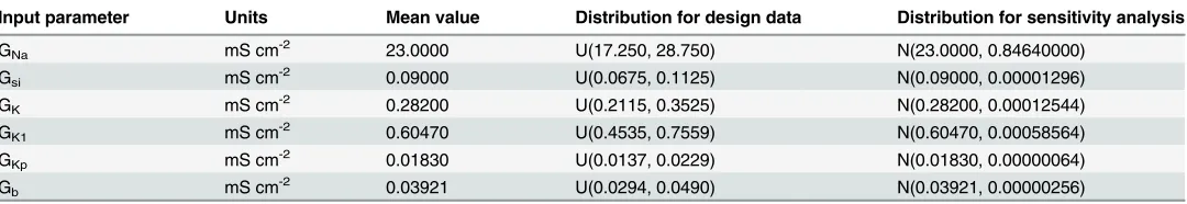
In the original description of the LR1991 model [26], values for the maximum conductances were chosen based on earlier models and on experimental data. Our aim was to use the emula-tor to undertake sensitivity analysis over a plausible region of model parameter space, rather than to chose inputs that represented beliefs (in a probabilistic sense) about the‘true’ mum conductances. For the design and test data, we therefore selected combinations of maxi-mum conductances using Latin hypercube sampling [27] from a uniform distribution in the rangeGxGx=4whereGxwas the maximum conductance provided in the original

descrip-tion of the LR1991 model. This range of parameters was chosen to avoid inputs (for example GK<0.2 mScm-2) that would generate prolonged repolarisation in the LR1991 model, and is shown inTable 1. The uniform distribution of each input was normalised to the range [0, 1] with the original conductance reported for the LR1991 model corresponding to 0.5. Thus normalised GNavaried from 0.0 corresponding to 17.25 mScm-2on the natural scale, to 1.0 corresponding to 28.75 mScm-2. For uncertainty and sensitivity analysis using the emulator, the inputs were assigned a Normal distribution with a mean of 0.5 and a variance of 0.04 (standard deviation 0.2) in normalised units. These values were chosen so as not to stray outside the range of the design data used to construct the emulators, and the mean and variance of each input in natural units is also given inTable 1.

the purpose of testing the emulator, and these data are also provided as Supporting Informa-tion (S2 Data). The choice of 200 for the number of design points was obtained empirically; fit-ting the emulators with design data based on<150 design points resulted in a relatively poor fit when evaluated against test data, whereas building an emulator with>250 design points resulted in a very similar fit to that obtained with 200 design points.

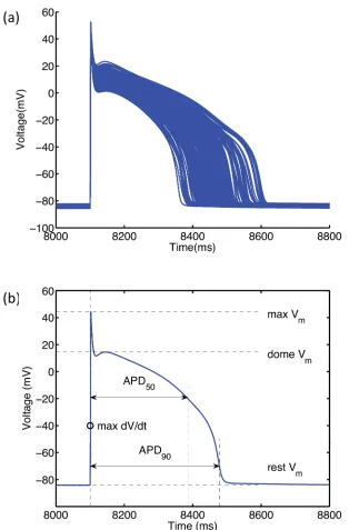
Each time the simulator was run (for generating both design and test data) nine S1 stimuli of strength -25.5μA cm-2and duration 2 ms were delivered to the simulator at a 1000 ms cycle length. The final action potential in this S1 sequence was used to obtain the outputs.Fig 1(a) shows the 200 action potentials that were used to generate the outputs.Fig 1(b)shows the six outputs that were measured directly from the action potential.

The slope of the APDr curve and minimum DI characterise dynamic properties of the simu-lator and were obtained as follows. Following the initial simusimu-lator run to obtain the outputs shown inFig 1(b), the simulator was run repeatedly using the final S1 beat of the initial run as an initial condition, with an S2 stimulus delivered at progressively shorter cycle lengths until an S2 beat could not be elicited. The stimulus strength and duration were -25.5μA cm-2and 2 ms as described above. From each of these additional runs, APD90and diastolic interval (DI) were obtained from the S2 action potential, and used to construct an APDr curve. The mini-mum DI was the shortest DI in the S2 sequence. The maximini-mum slope was determined by fitting an equation of the form

APD¼abeDI=c ð₁Þ

to the APDr curve using the Matlabfminsearchfunction, where a, b and c were obtained from thefit. The maximum slope of the curve was then determined [28] from

MaxSlope¼a be

DImin=b: ð₂Þ

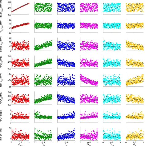
The design data inputs and outputs are plotted inFig 2, where each plot shows one of the eight output quantities plotted against one of the six input quantities. Test data are overlaid as dark grey points. Several associations are immediately clear from this figure, for example maxi-mum dVm/dT and peak Vmare both strongly associated with GNaand weakly associated, if at all, with the other inputs. On the other hand, APD90shows shows some dependence on Gsi, GK, and Gb. Note that the inputs have been normalised such that they to lie in the (0,1) interval. The uniform sampling distribution for the inputs is clear from the even spread of points in the (0,1) interval.

Table 1. Distribution for input parameters.

Input parameter Units Mean value Distribution for design data Distribution for sensitivity analysis

GNa mS cm-2 23.0000 U(17.250, 28.750) N(23.0000, 0.84640000)

Gsi mS cm-2 0.09000 U(0.0675, 0.1125) N(0.09000, 0.00001296)

GK mS cm-2 0.28200 U(0.2115, 0.3525) N(0.28200, 0.00012544)

GK1 mS cm-2 0.60470 U(0.4535, 0.7559) N(0.60470, 0.00058564)

GKp mS cm-2 0.01830 U(0.0137, 0.0229) N(0.01830, 0.00000064)

Gb mS cm-2 0.03921 U(0.0294, 0.0490) N(0.03921, 0.00000256)

Distribution for each input to the LR1991 simulator used for generating the design data and test data, and the distribution of each input used for undertaking sensitivity analysis in the emulator. U denotes a uniform distribution and N a normal distribution, with mean and variance given in brackets.

Building and evaluating the emulator

Our approach to Gaussian process emulator construction was based on that described in previ-ous studies [23,25], and a detailed description of the process and the underlying mathematics is given in the Supporting Information (S1 Text). We fitted a separate GP emulator for each of the eight outputs using the 200 sets of design data. Emulator fitting refers to the process of esti-mating emulator hyperparameters. In our study each emulator was characterised by a set of

Fig 1. Outputs produced by the LR91 model.(a) Action potential biomarkers used as model outputs to characterise the model. (b) Action potential time series from 200 runs of the LR1991 model used as design data for the GP emulator.

seven‘mean function’hyperparameters (an interceptb^0, and six slope hyperparameters

^

b1; :::;b^6corresponding to the inputs), and a set of seven‘covariance function’ hyperpara-meters (six correlation lengthsd^1; :::;d^6controlling the‘wiggliness’of the emulator, and an overall variance hyperparameter^s2). Given design data and hyperparameter values, an emula-tor can be evaluated for any new set of inputs. An emulaemula-tor evaluation for a new input is a Gaussian probability distribution with a defined mean and variance that represents our knowl-edge about the output of the simulator at that input.

Fig 2. Design data and test data obtained from 220 runs of the LR1991 model for eight outputs and six inputs.Each plot shows combinations of inputs and outputs, with 200 coloured points indicating design data used to fit the emulators, and 20 grey points showing test data used to validate the emulator.

The quality of the emulator fit was evaluated using the test data. The output distributions predicted by the emulator for the new inputs were compared with the actual outputs obtained from the simulator at the test points. A visual indication of fit was obtained by plotting the dif-ferences between the emulator means and the simulator outputs for each of the 20 test data points, and a quantitative indication was obtained by combining these differences into a single measure, the Mahanalobis distance (MD). This measure provides a robust way to compare the output of the emulator and the output of the simulator at the test points, expressed as a single number [29]. A reference distribution for the MD can be calculated, which for 20 points has a mean of 20 and a standard deviation of 6.8 [29]. A good quality emulator fit will predict the output at the test points correctly, and the MD will be close to the mean of the reference distribution.

When a satisfactory emulator fit had been obtained, the test data were then combined with the original design data and used to fit an updated emulator based on 220 simulator runs.

Uncertainty analysis

Uncertainty analysis aims to quantify how uncertain we are about the target output quantity, given our uncertainty about the model inputs. The traditional approach to this problem is Monte Carlo analysis, whereby a large number of samples is generated from the input parame-ter distribution, and for each sample the model is run. The resulting set of model outputs repre-sents a sample from a distribution that characterises the uncertainty about the output quantity. In contrast, an emulator can be used to specify directly an analytic distribution (in our case, a Gaussian process) that represents uncertainty about the output, given uncertainty in the inputs [30].

Sensitivity analysis

For the purposes of our study, we assumed that uncertain inputs are normally distributed, and under this assumption we can derive analytically a range of sensitivity analysis measures that quantify the effect of individual inputs on each output (seeS1 Textfor details). In particular, we can determine the inputs that have the greatest (and least) influence on an output, thereby giving insight into the operation of our model. Without an emulator, these sensitivity measures would typically require a costly Monte Carlo procedure.

The emulator was used to assess the contribution of each input with respect to each output inmean effectplots (a plot of the expectation of the output quantity, conditional on the input of interest, plotted against the input of interest), and to calculate themain effect index, for each input-output combination [23,30]. Sensitivity measures computed using the Gaussian process emulator were then compared with those computed using a PLS emulator [19] constructed using the same design data. The mathematical details of these procedures are described in detail in the Supporting Information (S1 Text), and are summarised here.

Themean effectof an input of interest, xw, on some output is the conditional expectation of that output, conditional on the input of interest, i.e. after averaging over the remaining inputs. This is a function of the given input xw, and enables the effect of varying a single input on the output to be examined. In each emulator, the mean effect of each of the six inputs was calcu-lated in turn over the range 0!xw!1, with all other inputs independently normally

distrib-uted with mean 0.5 and variance 0.04. A variance of 0.04 was chosen so that input values had good coverage over the (0,1) interval.

model outputVar{f(x}. If, by the variance identity, we writeVar{f(x} =Var[E{f(x)jxw}]+E[Var

{f(x)jxw}], we can see that the main effect index can be interpreted as the expected reduction in

variance in the output that would occur if we were to learn (or fix) xw.

Again, because we used an emulator to calculate the sensitivity measure we took expecta-tions with respect to the emulator, and calculated the ratio of the emulator expectation of the mean effect varianceE[Vw] to the emulator expectation of the variance of the emulator output E[Var[f(x)]]. The main effect index does not take into account any variance in the output that could be attributed to interactions between the inputs. However, in the absence of interactions the sum of the sensitivity indices for each input will be 1.0, and deviation from this is therefore a measure of the contribution of interactions.

The PLS emulator was generated following Sobie [19] using the NIPALS algorithm [31]. The combined design and test data used to fit the GP emulator were used to generate the PLS emulator. Inputs were first mean centred and normalised by the standard deviation to obtain Z scores. The Z scores of the input X, and the columns in output Y corresponding to APD90and maximum dVm/dT were then log-transformed. The eight outputs were then regressed on the six inputs resulting in 8 × 6 regression coefficients.

Results

APD90

emulator

To explain the way that GP emulators were used in this study, we concentrate initially on the APD90emulator, before presenting our findings for the other emulators.

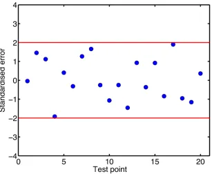
The evaluation of the APD90emulator against test data is shown inFig 3, which shows the difference between the output of the emulator and the output of the simulator for each of the 20 test data. These differences all fall within ± 2 emulator standard deviations, indicating that the emulator is a good fit. The Mahalanobis Distance (MD) for these test data was 28.22, which is within the plausible range given the reference distribution (mean 20 and standard deviation 6.8) [29]. See the Supporting Information (S1 Text) for details of how the MD was calculated. We therefore concluded that the APD90emulator was a good representation of the simulator.

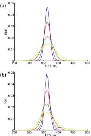
We next assessed how the variance of APD90calculated directly using the emulator

depended on the variance of GK. For this calculation, all inputs except GKwere effectively fixed by assigning independent normal distributions with a mean in normalised units of 0.5 and a very small variance of 0.0001 in normalised units. GKwas then assigned a normal distribution with mean 0.5 in normalised units (0.282 mS cm-2on the natural scale), but to show the effect of increasing uncertainty in GK, the variance was set at 0.01, 0.02, 0.05 and 0.1 in successive calculations of the mean and variance of APD90. These normalised variances correspond to standard deviations of 0.0014, 0.0028, 0.0071, and 0.0141 mS cm-2on the natural scale. The output distributions of APD90for each distribution of GKare shown inFig 4(a). As would be expected, increasing the variance of GKresults in an increase in the variance of APD90.

was therefore more efficient. The emulator approach (Fig 4(a)) required 220 simulator runs to generate design and test data, and once the emulator had been built (which took several min-utes), the calculation of each new output distribution took only a few seconds. In contrast, each distribution of the Monte Carlo based approach (Fig 4(b)) was calculated from 2000 simulator runs (an order of magnitude more). While this study did not undertake a full benchmark com-parison, we noted that computation times for each Monte Carlo run of 2000 samples varied from 9 hours 13 min to 9 hours 34 min.

Figs5and6show the result of sensitivity analysis using the APD90emulator.Fig 5shows the mean effects, which are the conditional expectation of the output, as each input in turn was fixed and varied from 0 to 1, while all other inputs were assigned a mean of 0.5 and a variance of 0.04. Increasing GK, Gb, and GK1above their mean value of 0.5 acted to decrease mean APD90in the emulator, whereas increasing Gsiabove 0.5 acted to increase mean APD90. These observations are consistent with the operation of the LR1991 model, where GK, Gb, and GK1 control outward depolarising currents, and Gsicontrols an inward depolarising current. 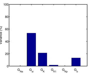The trends shown inFig 5can also be seen in the scatter plots of the design data inFig 2.

Fig 6shows the main effect index (expressed as a percentage) from the APD90emulator for each of the six inputs. We can interpret the main effect index as being the proportional reduc-tion in variance of APD90that would be expected if the input in question was to be fixed. The analysis confirms that Gsi, GK, and Gbwere the most important parameters for determining variability in APD90. The sum of these sensitivity indices was 98.4%, indicating that most of the total variance in APD90could be accounted for by the independent effects of variance in the inputs.

Fig 3. Validation of APD90emulator output against test data output.This plot shows the difference in the mean APD90predicted by the emulator and APD90obtained from the simulator for each of the 20 test data.

The difference is calibrated as the number of standard deviations, and the red lines indicate±2 standard deviations.

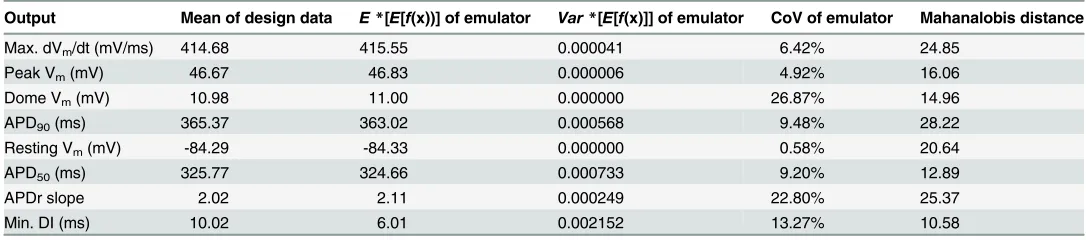
Design data characteristics and evaluation for all emulators

The design data and characteristics of each emulator are given inTable 2, where all inputs were independently normally distributed with a normalised mean of 0.5 and variance of 0.04 (see Table 1for natural units). In each case, the mean emulator outputE[E{f(x)}] was close to the mean of the simulator output in the design data for each of the emulators, and the variance of the mean emulator outputVar[E{f(x)}] was small, indicating that there little uncertainty was

Fig 4. Variance in APD90emulator.(a) Distributions of APD90resulting from normal distributions of GK

when all other maximum conductances were effectively held constant by assigning a mean of 0.5 and a very small variance of 0.0001 in normalised units. GKwas assigned a mean value of 0.282 mS cm-2and variance

0.0014 (blue) 0.0028 (red), 0.0071 (green), 0.0141 (yellow) mS cm-2_{. (b) Distributions of APD}

90obtained from

four Monte Carlo analyses, each with 2000 simulator runs, and with GKdrawn from distributions with mean

value of 0.282 mS cm-2and variance 0.0014 (blue) 0.0028 (red), 0.0071 (green), 0.0141 (yellow) mS cm-2.

Fig 5. Mean effects in APD90emulator.Mean effect of each of the inputs on APD90as each input is varied

whilst the others are held at their mean value.

doi:10.1371/journal.pone.0130252.g005

Fig 6. Sensitivity indices in APD90emulator.Sensitivity index of each of the inputs on APD90, showing the

proportion of total variance that can be attributed to variance in each input.

induced in the emulator fit. The coefficient of variation in the emulator output was obtained by dividing the square root of the emulator expectation of the varianceE[Var{f(x)}] by the emu-lator expectation of the expectation of the simuemu-lator outputE[E{f(x)}]. The MD obtained from the initial emulator fit is also given (seeS1 Textfor details of the MD calculation). In each case, the MD was within ±2 standard deviations of the reference distribution mean, and so the emulators were considered a good fit to the design data.

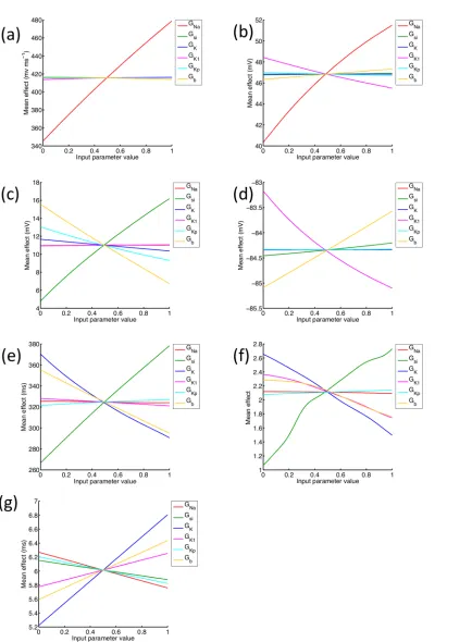
Mean effects in all emulators

The mean effects obtained using the emulator for each output are shown inFig 7. In the LR1991 model the action potential upstroke is controlled by INa, and the Max. dVm/dt and Max. Vmemulators have captured a strong dependence on GNaas shown in Fig7(a)and7(b). Dome voltage (Fig 7(c)) was mainly influenced by Gsiand Gb, with increasing Gsiacting to increase dome voltage, and Gband to a lesser extent GKpacting in the opposite direction. In the LR1991 model these effects reflect the balance of inward and outward currents during the action potential plateau. Changes in resting voltage (Fig 7(d)) were small, and were controlled by Gband GK1, while the mean effects for the APD50emulator (Fig 7(e)) were very similar to those of the APD90emulator (Fig 4), as well as the trends in the design data (Fig 2).

APDr slope is important for the stability of re-entry in cardiac tissue, and the mean effects plot for APDr slope (Fig 7(f)) shows that increasing Gsiacted to increase APDr slope, while increasing GK, GK1and Gbacted to decrease the slope. The dependence of APDr slope on Gsi, GK, GK1and Gbwas similar to the dependence of APD, and is also consistent with other studies of re-entry that have used the LR1991 model, where Gsihas been used to control the slope of the APD restitution curve [32,33].

Variance based sensitivity analysis

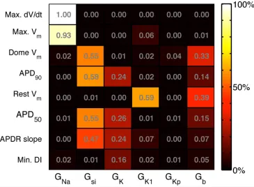
Fig 8shows the main effect indices calculated for each input, and for each emulator. These indices mirror the information shown in the mean effects plots, and indicate, for example, that GK1and Gbare the inputs that had the most influence on resting voltage. The sum of the main effect indices for was close to 1 (>98%) for all outputs except the APDr (85%) and the

Table 2. Emulator characteristics.

Output Mean of design data E*[E[f(x))] of emulator Var*[E[f(x)]] of emulator CoV of emulator Mahanalobis distance

Max. dVm/dt (mV/ms) 414.68 415.55 0.000041 6.42% 24.85

Peak Vm(mV) 46.67 46.83 0.000006 4.92% 16.06

Dome Vm(mV) 10.98 11.00 0.000000 26.87% 14.96

APD90(ms) 365.37 363.02 0.000568 9.48% 28.22

Resting Vm(mV) -84.29 -84.33 0.000000 0.58% 20.64

APD50(ms) 325.77 324.66 0.000733 9.20% 12.89

APDr slope 2.02 2.11 0.000249 22.80% 25.37

Min. DI (ms) 10.02 6.01 0.002152 13.27% 10.58

For each of the outputs, column 2 shows the mean of the design data, obtained from inputs that varied across the normalised range 0..1 given inTable 1. Columns 3-5 show the expectation of emulator output (_E*[_E[_f(x))]), the variance of this expectation_Var*[_E(_f(x))], and coef_ficient of variation

(pffiffiffiffiffiffiffiffiffiffiffiffiffiffiffiffiffiffiffiffiffiffiffiffiffiffiffiE_{½VarðfðxÞÞ=E½E½fðxÞ 100) of each emulator, when all of the inputs were assigned a standardised mean of 0.5, and a standardised variance of} 0.04 (i.e. 95% confidence intervals of 0.108 - 0.892). Column 7 shows the Mahanalobis distance between eachfitted emulator and an additional 20 test points; a goodfit was indicated by a value falling in a distribution with a mean of 20 and a standard deviation of 6.8.

Fig 7. Mean effects in each emulator.Mean effect of each of the inputs on each output as each input is varied whilst the others are held at their mean value.

minimum DI (26%). These lower values indicate that 15% of the APDr emulator variance and 74% of the minimum DI emulator variance could be accounted for by interaction effects.

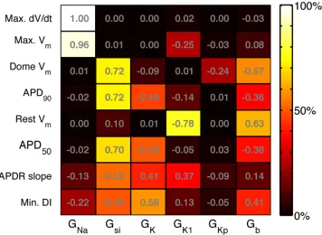
To provide a comparison with the main effects indices obtained from the GP emulators and shown inFig 8, we also calculated regression coefficients for the LR1991 model using partial least squares (PLS) regression [19]. These coefficients were obtained from the design and test data used to construct the GP emulators, and are shown inFig 9. These regression coefficients indicate how each output change with each input. Positive values indicate that the output increases as the input increases, whereas negative values indicate that the output decreases as the input increases. The PLS regression coefficients and main effects indices obtained from the GP emulators provide different ways of assessing the way that inputs affect outputs. However the magnitude of the PLS regression coefficients showed good agreement with the main effects indices from the GP emulators. Similar PLS regression coefficients could be obtained using alternative design data drawn from multivariate normal distributions rather than the uniform distribution of the combined design and test data used to construct the GP emulators.

Discussion

Summary of findings

In this study we have built a surrogate statistical model of the LR1991 cardiac cell model using, for each model output, a Gaussian process (GP) emulator. The emulators were used to under-take uncertainty and sensitivity analyses of the model efficiently. We found that the GP emula-tors could be fitted well given a small number of design data points, and we have shown that an

Fig 8. Variance based main effect indices for each emulator.Main effect index of each emulator (rows) to each input (columns), describing the proportion of the output variance that can be accounted for by variance on the input.

emulator approach is a powerful tool for uncertainty and sensitivity analysis in cardiac cell models.

The sensitivity indices shown in Figs8and9are consistent with what would be expected from our knowledge of the LR1991 model and the underlying physiology that the model repre-sents. They confirm that both GP and PLS emulators have captured the model behaviour cor-rectly. For example, GNacontrols the magnitude of the input current during the action potential upstroke, and so would be expected to have a strong influence on maximum dVm/dt and peak Vm. This association is seen in the design data (Fig 2), and the high sensitivity indices in Figs8and9show that this behaviour has been captured by the emulators. Similarly, Gsiand GKcontrol the input and output currents during the action potential plateau and repolarisation in the LR1991 model, and so would be expected to influence APD90. This association is again seen in the sensitivity indices in Figs8and9.

In the present proof of concept study, we have not attempted to assign uncertainty to the model inputs based on real uncertainties based on experimental errors and variation. However, an important future direction of this research will be to apply an emulator approach to biophy-sically detailed cell models, where the uncertainty in the mode inputs is based on variability in experimental data.

Comparison with other approaches

Some of the dependence of outputs on inputs identified with the emulators can be seen in the design data plotted inFig 2. These data show some of the relationships that are revealed by sen-sitivity analysis, but other relationships are obscured. For example, although the dependence of

Fig 9. Sensitivity indices calculated with PLS technique.Sensitivity index of each emulator (rows) to each input (columns).

Max. dVm/dt and Max. Vmon Gsiis clear fromFig 2, the relative influence of GK, Gsiand Gb on APD90is hard to quantify from these data alone.

Several recent studies have addressed the problem of parameter sensitivity in cardiac cell models by running large numbers of simulations, where parameters used for each simulation are drawn from a prescribed distribution [12,17,18]. Monte Carlo analysis has become one of the standard tools for undertaking sensitivity analysis. However a key advantage of an emulator based approach that is it less computationally demanding. In the present study 220 simulator runs were used to build all of the emulators, and the mean and variance of each emulator out-put could be calculated directly. In contrast, the Monte Carlo simulations used to generate the comparable data shown inFig 4(b)required 8000 simulator runs and took several days to com-pute. Thus an emulator based approach provides a computationally cheaper and more flexible way to examine the sensitivity of a cardiac cell model than‘brute force’Monte Carlo.

There are many different ways to build an emulator of a complex model, and other recent studies have used partial least squares (PLS) regression to build emulators that can be used for sensitivity analysis [19,20]. The sensitivity indices obtained by this approach (Fig 9) identify similar dependencies of outputs on parameters, although the methodology by which the two sets of indices are calculated is different and so there are some quantitative differences. An important benefit of the GP emulator approach over a PLS approach is that uncertainties in inputs are handled explicitly, and so it is possible to examine how the variance of an output changes as an input becomes more uncertain (Fig 4).

Assumptions, limitations, and difficulties of fitting GP emulators

Although GP emulators are a efficient and powerful tools for uncertainty and sensitivity analy-sis, the approach described in this study does involve several important assumptions. First, each output is assumed to be a smooth function of the inputs without discontinuities. This assumption was reasonable for most of the emulators examined in the present study, but may underlie problems with the Min. DI emulator and this issue is discussed in more detail below. Second, it is important that the design data fill the input space evenly. In this study we used a Latin hypercube design to ensure an even distribution of the inputs, and selected the number of design points empirically. We did not undertake a systematic assessment of the minimum number of design points needed to specify each emulator, and this is a topic for future studies with more biophysically detailed cardiac cell models. In addition, other approaches such as orthogonal sampling may provide a more efficient way to cover the parameter space [34].

Third, in this study each GP was described by a linear mean and a Gaussian form for the covariance. As described inS1 Text, this approach enables the direct calculation of integrals involved in the uncertainty and sensitivity analysis. All of the emulators performed well when evaluated with the test data, indicating that our choice of form was satisfactory.

A final assumption was that uncertainty in the emulator inputs and outputs was normally distributed. Experimental data used to construct cardiac cell models are usually assumed to be normally distributed, and are plotted with symmetric error bars [7]. In the present study we did not attempt to estimate the actual uncertainty in inputs because LR1991 is a simplified and generic model. However future studies of more detailed cardiac cell models could assign uncer-tainties to the inputs that are based on variability in the experimental data used to construct the model, and this would produce valuable insight into the model building process.

discontinuity in Min. DI in the input space, and careful examination of the design and test data plotted inFig 2shows possible evidence of a discontinuity in the dependence of Min. DI on Gsi. However, the sensitivity indices from the PLS emulator shown inFig 9were derived from the same design data, and indicate that Min. DI depends mainly on Gsi, GK, and Gb, a tendency also visible inFig 8although the absolute values are much smaller. It is possible that Min. DI is influenced by interactions between these inputs, and this would not be accounted for in the sensitivity indices shown inFig 8.

Conclusions

In this proof of concept study, we have shown that GP emulators can be used for uncertainty and sensitivity analysis in a model of the cardiac cell action potential. We chose an old and sim-plified model for this study because its operation is well understood compared to more recent biophysically detailed cell models. We expect that future studies will examine these more detailed models, and will explore the use of GP emulators for uncertainty analysis in multiscale models of cardiac electrophysiology.

Supporting Information

S1 Text. Additional mathematical details.Detailed description of the Gaussian process emu-lator, how the design data were used to fit the emuemu-lator, how the emulator was evaluated, and how it was used for variance based sensitivity analysis.

(PDF)

S1 Data. Design data.Design data used to fit the emulators. Data file in comma separated value format with 200 rows, each representing one simulator run. The first 6 columns are the inputs (parameters) in normalised units, and the subsequent columns are the eight outputs. (CSV)

S2 Data. Test data.Test data used to evaluate the emulators. Data file in comma separated value format with 20 rows, each representing one simulator run. The first 6 columns are the inputs (parameters) in normalised units, and the subsequent columns are the eight outputs. (CSV)

Acknowledgments

The design and test data were produced using theicebergcompute resource at the University of Sheffield. We also thank Jeremy Oakley (Sheffield) for helpful discussions.

Author Contributions

Conceived and designed the experiments: RC EC. Performed the experiments: RC EC. Ana-lyzed the data: RC EC MS. Contributed reagents/materials/analysis tools: MS. Wrote the paper: RC EC MS.

References

1. Noble D (1962) A modification of the Hodgkin-Huxley equations applicable to Purkinje fibre action and pacemaker potentials. Journal of Physiology (London) 160: 317–352. doi:10.1113/jphysiol.1962. sp006849

3. Mirams GR, Davies MR, Cui Y, Kohl P, Noble D (2012) Application of cardiac electrophysiology simula-tions to pro-arrhythmic safety testing. British Journal of Pharmacology 167: 932–45. doi:10.1111/j. 1476-5381.2012.02020.xPMID:22568589

4. Fink M, Niederer SA, Cherry EM, Fenton FH, Koivumaki JT, Seemann G, et al. (2011) Cardiac cell modelling: Observations from the heart of the cardiac physiome project. Progress in Biophysics and Molecular Biology 104: 2–21. doi:10.1016/j.pbiomolbio.2010.03.002PMID:20303361

5. Colman MA, Aslanidi OV, Kharche S, Boyett MR, Garratt CJ, Hancox JC, et al. (2013) Pro-arrhythmo-genic Effects of Atrial Fibrillation Induced Electrical Remodelling- Insights from 3D Virtual Human Atria. Journal of Physiology (London) 17: 4249–4272. doi:10.1113/jphysiol.2013.254987

6. ten Tusscher KHWJ, Panfilov AV, Tusscher KT (2006) Alternans and spiral breakup in a human ventric-ular tissue model. American Journal of Physiology (Heart and Circulatory Physiology) 291: 1088– 1100. doi:10.1152/ajpheart.00109.2006

7. O_’Hara T, Virág L, Varró A, Rudy Y (2011) Simulation of the undiseased human cardiac ventricular action potential: model formulation and experimental validation. PLoS Computational Biology 7: e1002061. doi:10.1371/journal.pcbi.1002061PMID:21637795

8. Clayton RH, Bernus O, Cherry EM, Dierckx H, Fenton FH, Mirabella L, et al. (2011) Models of cardiac tissue electrophysiology: Progress, challenges and open questions. Progress in Biophysics and Molec-ular Biology 104: 22–48. doi:10.1016/j.pbiomolbio.2010.05.008PMID:20553746

9. Rantner L, Tice B, Trayanova NA (2013) Terminating ventricular tachyarrhythmias using far-field low-voltage stimuli: Mechanisms and delivery protocols. Heart Rhythm 10: 1209–1217. doi:10.1016/j. hrthm.2013.04.027PMID:23628521

10. Hodgkin A, Huxley A (1952) A quantitative description of membrane current and its application to con-duction and excitation in nerve. Journal of Physiology (London) 117: 500–544. doi:10.1113/jphysiol. 1952.sp004764

11. Niederer SA, Fink M, Noble D, Smith NP (2009) A meta-analysis of cardiac electrophysiology computa-tional models. Experimental Physiology 94: 486–95. doi:10.1113/expphysiol.2008.044610PMID: 19139063

12. Britton OJ, Bueno-Orovio A, Van Ammel K, Lu HR, Towart R, Gallacher DJ, et al. (2013) Experimentally calibrated population of models predicts and explains intersubject variability in cardiac cellular electro-physiology. Proceedings of the National Academy of Sciences of the United States of America 110: E2098–105.

13. Davies MR, Mistry HB, Hussein L, Pollard CE, Valentin JP, Swinton J, et al. (2012) An in silico canine cardiac midmyocardial action potential duration model as a tool for early drug safety assessment. American Journal of Physiology (Heart and Circulatory Physiology) 302: H1466–80. doi:10.1152/ ajpheart.00808.2011

14. Gaborit N, Le Bouter S, Szuts V, Varro A, Escande D, Nattel S, et al. (2007) Regional and tissue spe-cific transcript signatures of ion channel genes in the non-diseased human heart. Journal of Physiology (London) 582: 675_–93. doi:10.1113/jphysiol.2006.126714

15. Heijman J, Zaza A, Johnson DM, Rudy Y, Peeters RLM, Volders PG, et al. (2013) Determinants of beat-to-beat variability of repolarization duration in the canine ventricular myocyte: a computational analysis. PLoS Computational Biology 9: e1003202. doi:10.1371/journal.pcbi.1003202PMID: 23990775

16. Stewart P, Aslanidi OV, Noble D, Noble PJ, Boyett MR, Zhang H. (2009) Mathematical models of the electrical action potential of Purkinje fibre cells. Philosophical Transactions of the Royal Society A: Mathematical, Physical and Engineering Sciences 367: 2225–55. doi:10.1098/rsta.2008.0283

17. Romero L, Pueyo E, Fink M, Rodríguez B (2009) Impact of ionic current variability on human ventricular cellular electrophysiology. American Journal of Physiology (Heart and Circulatory Physiology) 297: H1436–45. doi:10.1152/ajpheart.00263.2009

18. Kharche S, Lüdtke N, Panzeri S, Zhang H (2009) A global sensitivity index for biophysically detailed cardiac cell models: a computational approach. In: Ayache N, Delingette H, Sermesant M, editors, Functional Imaging and Modelling of the Heart (FIMH). Lecture Notes in Computer Science 5528, vol-ume 5528, pp. 366–375.

19. Sobie EA (2009) Parameter sensitivity analysis in electrophysiological models using multivariable regression. Biophysical Journal 96: 1264–74. doi:10.1016/j.bpj.2008.10.056PMID:19217846

20. Sarkar AX, Christini DJ, Sobie EA (2012) Exploiting mathematical models to illuminate electrophysio-logical variability between individuals. Journal of Physiology (London) 590: 2555_–67. doi:10.1113/ jphysiol.2011.223313

22. Oakley JE, O_’Hagan A (2002) Bayesian inference for the uncertainty distribution of computer model outputs. Biometrika 89: 769–784. doi:10.1093/biomet/89.4.769

23. Oakley JE, O’Hagan A (2004) Probabilistic sensitivity analysis of complex models: a Bayesian approach. Journal of the Royal Statistical Society: Series B (Statistical Methodology) 66: 751–769. doi: 10.1111/j.1467-9868.2004.05304.x

24. Vernon I, Goldstein M, Bower RG (2010) Galaxy formation: a Bayesian uncertainty analysis. Bayesian Analysis 5: 619_–669. doi:10.1214/10-BA524

25. Lee LA, Pringle KJ, Reddington CL, Mann GW, Stier P, Spracklen DV, et al. (2013) The magnitude and causes of uncertainty in global model simulations of cloud condensation nuclei. Atmospheric Chemistry and Physics 13: 8879–8914. doi:10.5194/acp-13-8879-2013

26. Luo CH, Rudy Y (1991) A model of the ventricular cardiac action potential. Depolarization, repolariza-tion, and their interaction. Circulation Research 68: 1501–1526. doi:10.1161/01.RES.68.6.1501 PMID:1709839

27. McKay MD, Beckman RJ, Conover WJ (1979) Comparison of three methods for selecting values of input variables in the analysis of output from a computer code. Technometrics 21: 239–245. doi:10. 2307/1268522

28. Nash MP, Bradley CP, Sutton PMI, Clayton RH, Kallis P, Hayward MP, et al. (2006) Whole heart action potential duration restitution properties in cardiac patients: a combined clinical and modelling study. Experimental Physiology 91: 339_–354. doi:10.1113/expphysiol.2005.031070PMID:16452121

29. Bastos LS, O’Hagan A (2009) Diagnostics for Gaussian Process Emulators. Technometrics 51: 425– 438. doi:10.1198/TECH.2009.08019

30. Becker W, Oakley JE, Surace C, Gili P, Rowson J, Worden K. (2012) Bayesian sensitivity analysis of a nonlinear finite element model. Mechanical Systems and Signal Processing 32: 18–31. doi:10.1016/j. ymssp.2012.03.009

31. Geladi P, Kowalski BR (1986) Partial least-squares regression: a tutorial. Analytica Chimica Acta 185: 1–17. doi:10.1016/0003-2670(86)80028-9

32. Garfinkel A, Kim YH, Voroshilovsky O, Qu Z, Kil JR, Lee MH, et al. (2000) Preventing ventricular fibrilla-tion by flattening cardiac restitufibrilla-tion. Proceedings of the Nafibrilla-tional Academy of Sciences of the United States of America 97: 6061–6066.

33. Qu Z, Kil J, Xie F, Garfinkel A, Weiss J (2000) Scroll wave dynamics in a three-dimensional cardiac tis-sue model: roles of restitution, thickness, and fiber rotation. Biophysical Journal 78: 2761–2775. doi: 10.1016/S0006-3495(00)76821-4PMID:10827961