How to select the most relevant 3D roughness parameters of a surface

(1)

White Rose Research Online URL for this paper:

http://eprints.whiterose.ac.uk/134679/

Version: Accepted Version

Article:

Deltombe, R, Kubiak, KJ orcid.org/0000-0002-6571-2530 and Bigerelle, M (2014) How to

select the most relevant 3D roughness parameters of a surface. Scanning, 36 (1). pp.

150-160. ISSN 0161-0457

https://doi.org/10.1002/sca.21113

© Wiley Periodicals, Inc. This is the peer reviewed version of the following article:

Deltombe, R. , Kubiak, K. J. and Bigerelle, M. (2014), How to select the most relevant 3D

roughness parameters of a surface. Scanning, 36: 150-160, which has been published in

final form at https://doi.org/10.1002/sca.21113. This article may be used for

non-commercial purposes in accordance with Wiley Terms and Conditions for

Self-Archiving. Uploaded in accordance with the publisher's self-archiving policy.

[email protected] https://eprints.whiterose.ac.uk/ Reuse

Items deposited in White Rose Research Online are protected by copyright, with all rights reserved unless indicated otherwise. They may be downloaded and/or printed for private study, or other acts as permitted by national copyright laws. The publisher or other rights holders may allow further reproduction and re-use of the full text version. This is indicated by the licence information on the White Rose Research Online record for the item.

Takedown

If you consider content in White Rose Research Online to be in breach of UK law, please notify us by

(2)

How to select the most relevant 3D roughness parameters of a surface

R. Deltombe*

1

, K.J. Kubiak

2,3

, M. Bigerelle

1,3

1_{Laboratoire LAMIH CNRS UMR, Université de Valenciennes et du Hainaut-Cambrésis, Valenciennes Cedex, France}

2_{School of Mechanical Engineering, iETSI, University of Leeds, UK}

3_{Laboratoire TEMPO EA4542, Université de Valenciennes et du Hainaut-Cambrésis, Valenciennes Cedex, France}

*

[email protected]

Summary:

In order to conduct a comprehensive roughness analysis, around sixty 3D roughness parameters are created to describe most of the surface morphology with regard to specific functions, properties or applications. In this paper, a multiscale surface topography decomposition method is proposed with application to stainless steel (AISI 304), which is processed by rolling at different fabrication stages and by electrical discharge tool machining. Fifty-six 3Droughness parameters defined in ISO, EUR, and ASME standards are calculated for the measured surfaces. Then, expert software “MesRug” is employed to perform statistical analysis on acquired data in order to find the most relevant parameters characterizing the effect of both processes (rolling and machining), and to determine the most appropriate scale of analysis. For the rolling process: The parameter Vmc (the Core Material Volume—defined as volume of material comprising the texture between heights corresponding to the material ratio values of p = 10% and q = 80%) computed at the scale of 3 mm is the most relevant parameter to characterize the cold rolling process. For the EDM Process, the best roughness parameter is SPD that represents the number of peaks per unit area after segmentation of a surface into motifs computed at the scale of 8 m.

Keywords: Sendzimir cold rolling, Electrical discharge machining, Surface roughness, 3D-roughness

parameters, Statistical analysis, Bootstrap method, ANOVA.

1 INTRODUCTION

In many engineering industrial applications, the precise characterization of surface roughness is of paramount importance because of its considerable influence on the functionality of manufactured products (Whitehouse 2011). To reduce the manufacturing cost, manufacturers are interested in developing simple and reliable control methodologies suitable for routine production environments, with a high degree of quantitative precision and data repeatability. The topographic method is by far the most implemented one in surface quality assessment of metallurgical or mechanical products. The roughness of machined surfaces is of prime importance across a very wide spectrum of technical and scientific activities; including not only tribologists and production engineers but also highway and aircraft engineers, hydrodynamicists and even bioengineers (Stout and Blunt 2000). In the particular cases of tribology, the surface roughness influences adhesion, brightness, wear, friction in wet or dry environment. (Yang 2008). Because of the increasing interests from science and industry, a proliferation of roughness parameters, possibly running into hundreds, has been triggered to describe the different kinds of surface morphology with regard to specific functions, properties or applications but also to characterize materials degradation submit to

(3)

2 THE MULTISCALE ANALYSES OF THE RELEVANCE OF SURFACE TOPOGRAPHY (MARST)

In this part, we will describe the MARST methodology via a simple example of cold rolling process to well appreciate the different steps of the methodology. Then, in section 3, a more realistic case will be treated.

2.1 Step 0: Experimental aspect, the cold rolling process

The studied rolling process is used to reduce austenitic stainless steel strip from 3 to 0.49 mm. The rolling mill is a Sendzimir stand made up with two work rolls (diameter lower than 100 mm) which speed in a range of 300 to 650 m·min−1. During the rolling process, the rolls maintain pressure on the strip in order to reduce its thickness. Furthermore, a rear tension and a front tension are applied on the strip in order to guide the strip correctly at the mill entry. The final thickness is obtained after 10 rolling passes, with reduction ratio decreasing from 25% to 10%. Before being cold rolled, the hot rolled strip must be treated in order to remove oxide scales (Mougin et al. 2003, Montmitonnet 2006). For that purpose, the strip is shot blasted and pickled in hydro chloric acid bath. These industrial processes have an impact on down-stream processes by modifying surface characteristics such as roughness and plastic behavior. Indeed, the first three rolling passes are critical in the "scrub" of surface flaws. The roughness gradient between sheet and blasted cylinder is important. Large crushing asperities occur but are constrained by the trapping of lubricant in the valleys (Huart et al 2004). Thus, in order to select the most relevant 3D roughness parameters, three specimens are extracted from the industrial process. The first is the original shot blasted strip, the second is after one pass and the last is after three passes.

2.2 Step 1: Roughness measurements

The white light interferometer (NewView 7300, Zygo) is used for characterizing and quantifying surface roughness. Optical resolutions of x20 Mirau objective used are 0.71µm for x, y axes based on Sparrow criteria which take into account the lens numerical aperture and 0.01µm for z axe. Indeed, spatial sampling based on camera pixel size (0.55µm) is lower than the optical resolution. The inspected surface area is 700µm by 525µm obtained by stitching of each single measurement with 20% overlap.

2.3 Step 2: The multiscale decomposition

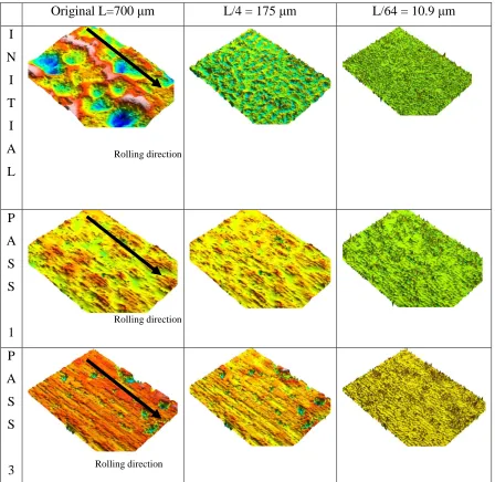
The Gaussian filter has been recommended by ISO 11562-1996 and ASME B46.1-1995 standards for determining the mean line in surface metrology. This filter was adapted in order to filter the 3D surfaces with a given cut off value (Yuan et al. 2000). In this study, only the high pass filter will be presented (for the sake of simplicity, we omitted the results of pass band filter because best parameters were not relevant in this study). Our system is used to filter all surfaces with different cut-off in order to obtain a multiscale decomposition. The 30 consecutive steps are used in this decomposition, with a cut-off varying from 2µm to 360µm. Figure 1 represents 2 high pass filters for the surface decomposition with two cut-off corresponding to L/4 and L/64 µm, L is the horizontal scanning length. When the cut-off decreases, microscopic details appear on filtered surfaces (Figure 1).

Then 3D Roughness parameters are computed. 3D roughness parameters are defined by the following standards: ISO 25178 define 30 parameters, EUR 15178N also define 30 parameters but some are identical to those of ISO 25178. Only 16 parameters are the latest ones, however Sz (maximum height of

surface roughness) and Std (texture direction) are

calculated differently in both standards. Further, 7 3D roughness parameters related to surface flatness are defined by ISO 12781, and ASME B46.1 define 7 similar parameters as ISO 25178 standard (with different predefined filters) and one new parameter SWt (area waviness height). This gives in total 56

different 3D roughness parameters, which will be considered in this study.

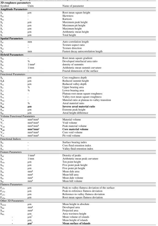
The 3D roughness parameters (see Table 1) can be classified into the following groups:

1. Amplitude parameters, 2. Spatial parameters, 3. Hybrid parameters, 4. Functional parameters, 5. Feature Parameters, 6. Other 3D parameters.

Figures 2a and 2b represent the changes of the two parameters Vmc and Smc versus decomposition scale

(the Gaussian filter cut off). It is observed that when the cut-off increases, lower frequencies on the surface are introduced and consequently the amplitudes of the parameters increase without regard to the process conditions. Because of the bootstrap analysis, it is noticed that the 3 process conditions present different values at different scales. However, the parameter Smc

presents a higher variation compared to Vmc. It can be

suggested that Vmc is more relevant to describe the

(4)

Original L=700 m

L/4 = 175 m

L/64 = 10.9 m

I

N

I

T

I

A

L

P

A

S

1 P

A

S

[image:4.595.75.523.46.482.2]

3

Figure 1. Cold rolled strip of AISI 304 measured before and after a first rolling process and after third rolling processes,

measured surface size 700 x 525 m. Examples of multiscale decomposition using Gaussian high pass filtering at cut off L/4 = 175 m and L/64 = 10.9 m.

2.4 Step 3: The measure of parameters relevancy by variance analysis

To measure the relevancy of the roughness parameters computed at a given spatial scale, an appropriate statistical tool will be used in the sequence. The most relevant scale is investigated by variance analysis, which is essentially an implementation of the generalized linear model. The formula is as follows:

( )

3

0 , ,

1

( , , )

,

j

i j k k n

j

p

ε

k n

α

i

ε ξ

i

ε

=

+

∑

+

(1)

where

p

i

( , , )

ε

k n

is value of the roughness

parameter of the

n

-th profile when the process parameters are taken at the k-th level (k denotes the initial surface after 1 rolling process, or after 3 rolling processes) for an evaluation length

ε

,

α

j,k_j

( )

i

,

ε

represents the influence on the roughness parameter

value of the j -th process parameter at the kj-th level.

( )

,

k n

i

ξ

ε

is a zero-mean Gaussian noise with standard deviation

σ

.

For each evaluation length, all of these influences are calculated by linear fitting. From them and for each process parameter and each interaction, between-group variability and within-between-group variability (corresponding to estimation errors of the roughness parameter of each group) are calculated. The result, denoted by

F

( )

p

i

,

ε

, is the ratio produced by

dividing the ‘between-group’ variability over the ‘within-group’ variability. In other words, this result compares the effect of each process parameter on the roughness parameter’s value with its estimation error. Consequently, for a given process parameter, a value of

F

( )

p

i

,

ε

near to 1 suggests an irrelevancy of the

roughness parameter

p

i estimated at the evaluation

Rolling direction

(5)

[image:5.595.47.560.57.787.2]

Table I: 3D roughness parameters calculated and analysed in this study.

3D roughness parameters

Symbol Units Name of parameter

Amplitude Parameters

Sq µm Root mean square height

Ssk - Skewness

Sku - Kurtosis

Sp µm Maximum peak height

Sv µm Maximum pit height

Sz µm Maximum height

Sa µm Arithmetic mean height

St µm Total height

Spatial Parameters

Sal mm Auto-correlation length

Str - Texture-aspect ratio

Std ° Texture direction

Sal mm Fastest decay autocorrelation length

Hybrid Parameters

Sdq - Root mean square gradient

Sdr % Developed interfacial area ratio

Sds 1/mm² density of summits

Ssc 1/mm Arithmetic mean summit curvature

Sfd - Fractal dimension of the surface

Functional Parameters

Sk µm Core roughness depth

Spk µm Reduced summit height

Svk µm Reduced valley depth

Sr1 % Upper bearing area

Sr2 % Lower bearing area

Spq - Plateau root mean square roughness

Svq - Valley root mean square roughness

Smq - Material ratio at plateau-to-valley transition

Smr % Areal material ratio

Smc µm Inverse areal material ratio

Sxp µm Extreme peak height

Sdc µm Areal height difference

Volume Functional Parameters

Vm mm³/mm² Material volume

Vv mm³/mm² Void volume

Vmp mm³/mm² Peak material volume

Vmc mm³/mm² Core material volume

Vvc mm³/mm² Core void volume

Vvv mm³/mm² Pit void volume

Functional Indices

Sbi - Surface bearing index

Sci - Core fluid retention index

Svi - Valley fluid retention index

Feature Parameters

Spd 1/mm² Density of peaks

Spc 1/mm Arithmetic mean peak curvature

S10z µm Ten point height

S5p µm Five point peak height

S5v µm Five point pit height

Sda mm² Mean dale area

Sha mm² Mean hill area

Sdv mm³ Mean dale volume

Shv mm³ Mean hill volume

Flatness Parameters

FLTt µm Peak-to-valley flatness deviation of the surface

FLTp µm Peak-to-reference flatness deviation

FLTv µm Reference-to-valley flatness deviation

FLTq µm Root mean square flatness deviation

Other 3D Parameters

Smean µm Mean height in absolute

Sdar mm² Developed area

Spar mm² Projected area

SWt µm Area waviness height

- µm3 _{Mean volume of islands}

- µm Mean height of islands

(6)

Decomposition scale (µm) Vm c (m m 3/m m 2)

2 4 6 8 12 18 25 38 53 77 116 175 350

0.025 0.050 0.075 0.250 0.500 0.750 2.500 5.000 7.500

Surface after 1 rolling process Surface after 3 rolling processes Initial surface

L/64 L/4

(a)

Decomposition scale (µm)

Sm

c

(

m

)

2 4 6 8 12 18 25 38 53 77 116 175 350

0 2 4 6 8 10 12 14 16

[image:6.595.53.283.45.417.2]

(b)

Figure 2. Evolution of the Core materials volume, Vmc (a)

and the relative material ratio ,Smc (b) versus the scale

(filter cut off) corresponding to the three surface topographies described in Figure 1.

length

ε

to represent effects of the process parameter in consideration. Higher the value of

F

( )

p

i

,

ε

is,

more relevant the parameter

p

iestimated at the scale

ε

becomes (see Van Gorp et al. 2010 for more details). In this way, we can compare not only

( )

p

i

,

ε

F

with regard to the evaluation length but also to the chosen roughness parameter. By checking the highest value of

F

( )

p

i

,

ε

, the most pertinent

roughness parameter and its evaluation length can be selected to describe the influence of a given process parameter. In the case of a cold rolling process, Figure 3 presents the changes of F

(

p_i,

ε

)

versus the evaluation length for 3 roughness parameters: Vmc,

Smc and Sha. By analyzing these figures, it can be

concluded that:

• Relevance is better for Vmc when it is

estimated at the low spatial scale of 3µm (microscopic scale).

• The relevance of Smc is quite constant at all

scales, does not depend on the scale and is less pertinent compared to Vmc.

• The mean of a island surface is very relevant at a higher spatial scale (around 350µm, macroscopic scale) and appears to be a characteristic length of the tool processing, however physical meaning of this parameter remains questionable especially at a higher decomposition scale.

R e le v a n c e f u n c ti o n F (p i , ε )

2.5 7.5 25 75 250

0.5 5.0 50.0 500.0 5000.0 50000.0 Mean Surface of islands Vmc Smc

Figure 3. Evolution of the relevancy criterion F for Core

materials volume Vmc, the relative material ratio Smc and

the mean surface of island versus the scale (filter cut off) to discriminate the three surface topographies described in Figure 1.

0 500 1000 1500 2000 2500 3000 3500 4000 4500

Classification order 0.005 0.050 0.500 5.000 50.000 500.000 5000.000 50000.000 R e le v a n c e f u n c ti o n More relevant Less relevant R e le v a n c e f u n c ti o n F (p i , ε ) 0.005 0.05 0.5 5 50 500 5000 50000

(a)

Best 3D roughness parameters

7000 8000 9000 10000 20000 30000 40000 50000 60000 70000 80000 900001E5 2E5 3E5

Median 25%-75% 5%-95%

The two best roughness parameters

Smc

Scale 3µm

Mean surface of islands Scale 200 µm

R e le v a n c e f u n c ti o n F (p i , ε )

(b)

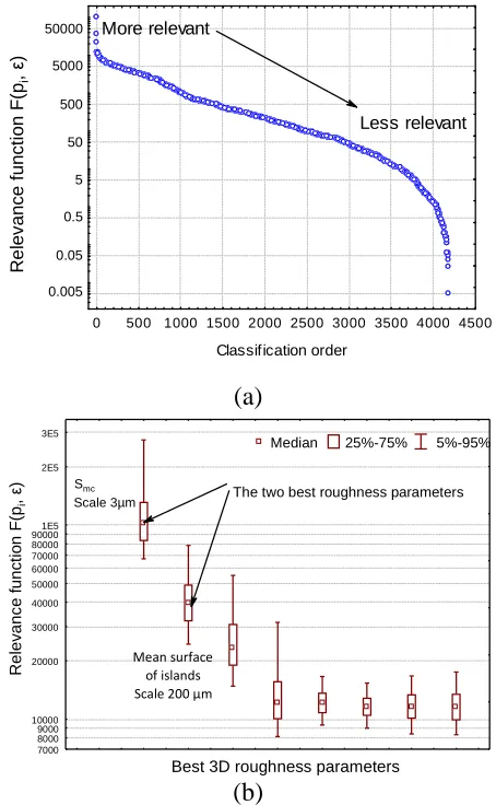
Figure 4. Classification of the 3D roughness Parameters

[image:6.595.311.542.128.328.2] [image:6.595.314.541.393.761.2]

(7)

surface topographies (a) described in Figure 1, (b) the most relevant parameters with their confidence intervals associated to the relevancy function F(pi, ε) obtained by bootstrap method.

In summary, these figures show that the range of relevant evaluation length depends on the type of roughness parameter. This multi-parameter representation of surface roughness has been reported in various works and some efforts have been put previously to develop a method for selecting relevant parameters (Scott et al. 2005, Narayan et al. 2006, Jordan et al. 2006, Berglund et al. 2010, Bigerelle et

al. 2005b).

2.5 Step 4: The classification of roughness parameters

It is possible to classify the relevancies of all parameters by classifying their F-values in descending order (Figure 4a). In order to include the robustness of the relevance of roughness parameters, bootstrap is used that allows estimating the error in the computation of the coefficients of statistical modeling. For these reasons, we shall introduce a recent technique called the bootstrap which is a resampling technique (Efron 1993, Hall 1992). The basic idea of the bootstrap is to create a new dataset by randomly sampling with replacement from the original data set and then performing the same statistical analysis as carried out on the original data set. This original bootstrap method applied to the analysis of variance allows obtaining variability on the F-values (Figure 4b).

The parameter Vmc is the most relevant one computed

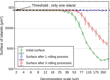
at the scale of 3µm and has the same relevance as the mean of the island surface measured at the scale of 300µm. The second most relevant roughness parameter is the “mean surface of islands” computed at the macroscopic scale roughness (300µm). Figure 5 shows that the discrimination of this parameter appears after a scale of 50µm and the threshold depends on the surface itself. An interesting property of the proposed method is that there is no meaningful correlation between Vmc and Sha and both parameters

describe different physical mechanisms.

2.6 Step 5: Bootstrap and Probability Density Function of the most relevant parameters

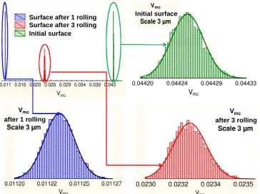
Once the most relevant 3D roughness parameter has been found, next step in the analysis is to calculate the mean Probability Density Function (PDF) of the most relevant parameters for the three processes considered in this study. Figure 6 represents the value of these PDF (histograms) of the roughness parameter Vmc for the three process conditions. It can be

observed that the relevance is very good because no

overlap appears and Vmc well discriminates the effect

conditions.

2.7 Final Step: Physical Interpretations of selected parameters

Initially, there are many valleys creating the space that are easily filled by the lubricant. After each consecutive rolling process, there are fewer voids for lubricant available. Due to the anisotropic texture along a rolling direction, the lubricant can leak outside the contact zone easily through the narrow network of valleys. The lubricant is supposed to flow according to the Couette equation having added the pressure gradient term (Stachowiak and al. 2005). The lubricant flows in the inlet area from valley to valley due to pressure gradient. Such a flow will be highly influenced by the roll and strip speeds. This is peculiarly true if the distance between each valley is small enough to create the flow. Furthermore at the roller entry, lubricant thickness is directly linked with rolling parameters. Thus, thickness is reduced as the bite angle increases and the speed is lower (Wilson and Walowit 1971).

This explains the decreasing tendency of the voids represented by Vmc. However, after three rolling

passes, voids volume tends to increase. Indeed, through the different passes, the lubricant hardly flows from valley to valley due to a sparse pits network. The only way for the lubricant to escape is at the inlet entry where the valley is squeezed out by roller. This effect decreases as roll speed is increasing and the roll bite angle is lower. It is expressed by Wilson and Walowit equation where the lubricant thickness tends to be higher as the strip thickness is reduced after every consecutive rolling process.

S u rf a c e o f is la n d s ( µ m 2)

2 4 6 8 12 18 25 38 53 77 116 175 350

500 5000 50000

5E5 Threshold : only one island

Figure 5. Evolution of the mean surface of islands versus

the decomposition scale (Gaussian filter cut off) corresponding to the three surface topographies described

[image:7.595.310.533.515.677.2]

(8)

Initial surface

Surface after 3 rolling

Surface after 1 rolling Initial surface

after 1 rolling after 3 rolling

Figure 6. Bootstrap histograms of the mean values of Vmc roughness parameters compute at the scale of 3 µ m for three

surface topographies described in Figure 1.

3 APLICATION OF THE MARST METHODOLOGY: CARACTERIZATION OF THE ELECTRICAL DISCHARGE MACHINING PROCESS

Isotropic topographies over a wide range of dimensions are tooled by Electrical Discharge Machining (EDM). The EDM process produces strongly isotropic, fractal and self-similar surfaces.

3.1 Step 0: Experimental aspect, the Electrical Discharge Machining (EDM)

21 different samples are tooled with EDM process, forming a very wide range of roughness whose amplitude Ra varies from 1.2µm to 15µm. The EDM:

a 5 mm thick plate of pure Titanium (Ti) was electro-eroded by EDM using a spark erosion machine provided by Charmilles (Switzerland). A copper electrode with a diameter of 20 mm was used with a tension of 220 V. Intensity and gap was controlled from 0.5 to 64A for intensity and from 0.02 to 0.25 mm for the gap (distance between sample and electrode) such as the first sample is the smoother and the last sample is the rougher. Then the plate was cut in order to obtain 21 samples with 21 roughness levels with an amplitude roughness parameter (Ra)

comprised between 1.2µm and 15µm (grades 1 to 21). X-ray Photoelectron Spectroscopy (XPS) analysis confirmed that the surface chemistry was identical for

all 21 samples and composed of titanium oxides (data not shown)

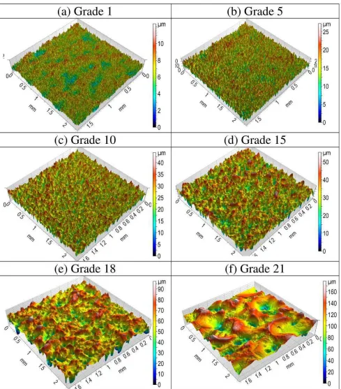
3.2 Step 1: Roughness measurements

Roughness Measurements: 3D roughness measurements were achieved on an Interferometer using a x20 objective (Zygo, USA). The axial resolution of the machine is around 10 nm and the plane resolution is around 710 nm (Figure 7). The surfaces obtained by electro-erosion present an isotropic structure formed by successive peaks and valleys. No specific direction or periodical structure is visible on surfaces. Higher the grade, higher the roughness amplitude, larger peaks-or-valleys.

3.3 Step 3 to 5: Core of the MARST analyses

Figure 8 represents the plot of the relevance of the first and second uncorrelated parameters. The best roughness parameter is Spd that represents the number

of peaks per unit area after segmentation of a surface into motifs (hills and dales). This segmentation is carried out in accordance with the watersheds algorithm. This parameter (ISO 25178) Spd replaces

the (EUR 15178N) parameter Sds. The peaks taken

into account for the (EUR 15178N) parameter Sds are

detected by local neighborhood (with respect to 8 neighboring points) without discrimination between local and significant peaks. The (ISO 25178) parameter Spd is calculated in the same way, but takes

[image:8.595.119.483.58.330.2]

(9)

[image:9.595.52.541.48.605.2]

(10)

Figure 8. Graph of relevance of the best pair of uncorrelated pair of roughness parameters Spd and Smean. Higher the Fisher

value, more relevant the roughness parameter.

of 5% of Sz). As it is shown, the MARST

methodology permits us to classify roughness parameters according to their relevancies. Another routine allows finding the roughness parameter that will be less correlated with the most relevant roughness parameter but keeping a high degree of relevance. Then, the second best relevance is obtained thanks to the use of the amplitude parameter Smean.

This parameter is complementary to Spd. MARST

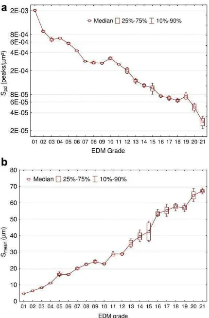
methodology has found that the two “uncorrelated” parameters are a frequency (one characterize by a number of peaks) and an amplitude (one characterize by a mean of maximal amplitude). From this analysis it is shown by figure 9, the following results can be stated:

• The lower the EDM grade (lower discharge power), the higher the peaks, but lower the maximal mean amplitude of the roughness. Higher discharges create highest peaks that decrease their numbers per unit area.

• However, some regime appears in this tendency with the number of the peaks formation and not really in the maximal amplitude of the roughness.

Figure 9. Value of the two best relevant roughness

parameters Spd (a, number of peaks) and Smean (b, maximal

[image:10.595.106.492.50.334.2] [image:10.595.309.524.384.711.2]

(11)

- A saturation of the mean amplitude for the highest grade (19 to 21) due to the weight of each droplet formed during discharge that will decrease its radius curvature and then amplitude.

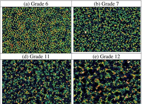
- A saturation appears for the number of peaks (during grade 7 to 11) and not for their associated amplitudes. This saturation is a transition due to peak percolation. To analyze this phenomenon, a morphological analysis will be performed on

[image:11.595.50.547.195.561.2]

peaks/valleys. The surface is vectorized by searching all the furrows contained on a surface. Figure 10 represents theses furrows before the threshold (grade 6), at the threshold (grade 7 to 11) and after the threshold (12). It can be observed that the number of peaks stays quite constant and is due to “depercolation” of the roughness, leading to a constant number of peaks during this process.

Figure 10. Vectorization of the furrows contained on EDM surfaces for four EDM grade.

4 CONCLUSION

This paper proposes a new and original methodology designed to select, without preconceived opinion, the 3D roughness parameters relevant for discriminating different topographies with regard to a specific application. Analysis of variance enabled to define and estimate a quantitative indicator for each roughness parameter and their associated decomposition scale. By using the recently developed Bootstrap method, it is possible to define and calculate a 90% confidence interval on the value of this indicator. Among 56 tested 3D roughness parameters, the results of this methodology revealed:

For the Rolling process: The Vmc parameter (the

Core Material Volume - defined as volume of material comprising the texture between heights corresponding to the material ratio values of p = 10% and q = 80%) is the most relevant parameter to characterize the cold rolling process. It is important to mention that the scale at which this parameter is the most relevant is 3 mm. This methodology allows understanding the mechanism of steel deformation during cold rolling and consecutive change of surface roughness after every rolling process.

(12)

surface into motifs computed at the scale of 8 m.

The most relevant parameters can be selected and used to control the quality of processes in manufacturing environment. Proposed methodology can be used to control other processes like tool’s wear evaluation, quality of produced paper, quality of machined surface, honed or polished surfaces. However, a complementary analysis must be performed in the future to gather the roughness parameters that are correlated.

5 ACKNOWLEDGEMENT

The fund is given by the region Picardie on the project FoncRug3D. The Mesrug team is composed of : Dr G. Guillemot (Software management, CetMef, Sofia Antipolis), Dr T.Correvitz (Metrology management, ENSAM, Lille), : Dr K. Anselme (Biological application, ICSI, Mulhouse), Pr A. Iost (Tool machining applications, LML, Lille), Dr. T. Mathia (Tribology and surface, LTDS, Lyon), Pr. J. Antony (signal processing, INSA, Lyon), Pr. A. Dubois (Machining tool processing, Tempo, Valenciennes), Dr. P. Revel (Metal processing, Roberval, Compiègne), Pr. A. Rassineux (Numerical optimization, Roberval, Compiègne), Dr. A. Jourani (tribology of contact, Roberval, Compiègne), Dr. B. Hagege (FEM simulation, Roberval, Compiègne), Pr. S. Bouvier (Mechanical properties, Roberval, Compiègne), Dr. D. Najjar (Corrosion, Ecole Centrale, Lille), Dr. P-E. Mazeran (Nano characterization, Roberval, Lyon), R. Vincent (metrology, Cetim, Senlis), S. Gabriel (Roughness ISO normalization, Cetim, Senlis), Dr. A Van Gorp (Surface measurement, Ensam, Lille), Dr. F. Bedoui (Polymer Science, Roberval, Compiègne), Dr. F. Henebelle (Surface coating, Univ Auxerre, Auxerre), Dr J.M. Nianga (Statistics, HEI, Lille), Dr. Jouini (tribology of tool processing, Univ Tunis, Tunis), A. Gautier (tool processing, BMW, Compiègne), Pr H. Migaud (Surgery and Biomechanics, CHRU, Lille), V. Duquenne (Secretaria, Roberval, Compiègne), S. Ho (Fatigue of Materials, Cetim, Senlis), Y. Xia (Hardness characterisation, Roberval, Compiègne), J. Marteau (Mechanical surface characterisation, Roberval, Compiègne). L. Dubar (Hot Metal Forming, Tempo, Valenciennes), Dr Giljean (Coating characterisation, ICSI, Mulhouse), Z. Khawaja (Computer Science, Roverval, Compiègne).

6 REFERENCES

ASME B46.1. 1995. Surface Texture: Surface Roughness. New York: Waviness, and Lay, American Society of Mechanical Engineers.

Berglund J., Brown C.A., Rosen B.G., Bay N. 2010. Milled die steel surface roughness correlation with steel sheet friction. CIRP Annals Manufacturing Technology 59(1): 577-580.

Bigerelle, M., Anselme, K. 2005. Bootstrap analysis of the relation between initial adhesive events and long-term cellular functions of human osteoblasts cultured on biocompatible metallic substrates. Acta Biomaterialia 1:499-510.

Bigerelle M., Gautier A., Iost A. 2007. Roughness characteristic length scales of micro-machined surfaces: A multi-scale modelling, Sensors and Actuators B: Chemical 126:126-137.

Efron B, Tibshirani RJ. 1993. An Introduction to the Bootstrap. New York: Chapman and Hall.

EUR 15178N. 1993. The development of methods for the characterisation of roughness in three dimensions", Stout, Sullivan, Dong, Mainsah, Luo, Mathia, Zahouani, Commission of the European Communities, EUR 15178 EN.

Hall P. 1992. The Bootstrap and the Edgeworth expansion. , New York: Springer-Verlag.

Huart S., Dubar M., Deltombe R., Dubois A., Dubar L. 2004. Asperity deformation, lubricant trapping and iron fines formation mechanism in cold rolling processes. Wear 257: 471-480.

ISO 11562: 1996, Geometrical Product Specifications (GPS) – Surface Texture: Profile Method -- Metrological Characteristics of Phase Correct Filters (International Organization for Standardization, Geneva, 1996).

ISO 25178-2:2012 Geometrical product specifications (GPS) - Surface texture: Areal - Part 2: Terms, definitions and surface texture parameters.

ISO 12781-1:2011 Geometrical Product Specifications (GPS) - Flatness - Part 1: Vocabulary and parameters of flatness.

(13)

Wear 261:398-409.

Montmitonnet P. 2006. Hot and cold strip rolling processes. Computer methods in applied mechanics and engineering 6604-6625.

Mougin J., Dupeux M. 2003. Adhesion of thermal oxide scales grown on ferritic stainless steels measured using the inverted blister test. Materials Science and Engineering A 359:44-51.

Najjar D., Bigerelle M., Iost A. 2003. The computer based Bootstrap method as a tool to select a relevant surface roughness parameter. Wear 254:450-460.

Najjar D., Bigerelle M., Migaud H., Iost A. 2006. About the relevance of roughness parameters used for characterizing worn femoral heads. Tribology Internationnal 39:1527-1537.

Narayan P., Hancock B., hamel R., Bergstrom T.S., Brown C.A. 2006. Differentiation of the surface topography of various pharmaceutical excipient compacts. Mat. Sci. Eng. A430(1-2):79-89.

Scott R.S., Ungar P.S., Bergstrom T.S., Brown C.A., Grine F.E., Teaford,, Walker A. 2005. Dental microwear texture analysis within-species diet variability in fossil hominins. Nature 205 436(4):693-695.

Stachowiak G. W., Batchelor A. 2005. Engineering tribology. 3 ed. Oxford: Elsevier Butterworth-Heinemann.

Stout K., Blunt L. 2000. Three-dimensional Surface Topography. 2 ed. London: Penton Press Van Gorp A., Bigerelle M., El Mansori M., Ghidossi

P., Iost A. 2010. Effects of Working Parameters on the Surface Roughness in Belt Grinding Process: the Size-scale Estimation Influence. Int. J. Mater. Prod. Tech. 38:66-77. Yang C. 2008. Role of Surface Roughness in

Tribology: From Atomic to Macroscopic Scaledfdfdfdfd. Berlin: GmbH.

Wilson W.R.D., Walowit J.A. 1971. An isothermal hydrodynamic lubrication theory for strip rolling with front and back tension. Tribol. Convection I. Mech. E C86171:164–172. Whitehouse D. J. 1982. The parameter rash — is

there a cure? Wear 83(1):75-78.

Whitehouse D. J. 2011. Handbook of Surface and Nanometrology, New York: CRC Press, Taylor & Francis.

Yuan Y. B., Vorburger T.V., Song J. F., Renegar T.