This is a repository copy of Comparing predictive accuracy in small samples. White Rose Research Online URL for this paper:
http://eprints.whiterose.ac.uk/90598/ Version: Published Version
Monograph:
Coroneo, Laura orcid.org/0000-0001-5740-9315 and Iacone, Fabrizio
orcid.org/0000-0002-2681-9036 (2015) Comparing predictive accuracy in small samples. Discussion Paper. Discussion Paper in Economics . Department of Economics and Related Studies, University of York
[email protected] https://eprints.whiterose.ac.uk/ Reuse
Items deposited in White Rose Research Online are protected by copyright, with all rights reserved unless indicated otherwise. They may be downloaded and/or printed for private study, or other acts as permitted by national copyright laws. The publisher or other rights holders may allow further reproduction and re-use of the full text version. This is indicated by the licence information on the White Rose Research Online record for the item.
Takedown
If you consider content in White Rose Research Online to be in breach of UK law, please notify us by
Discussion Papers in Economics
Department of Economics and Related Studies University of York
Heslington York, YO10 5DD
No. 15/15
Comparing predictive accuracy in small samples
Comparing predictive accuracy in small samples
Laura Coroneo
∗University of York
Fabrizio Iacone
University of York
September 14, 2015
Abstract
We consider fixed-b and fixed-m asymptotics for the Diebold and Mariano (1995)
test of predictive accuracy. We show that this approach allows to obtain pre-dictive accuracy tests that are correctly sized even in small samples. We apply the alternative asympotics for the Diebold and Mariano (1995) test to evaluate the predictive accuracy of the Survey of Professional Forecasters (SPF) against a simple random walk. Our results show that the predictive ability of the SPF was partially spurious, especially in the last decade.
Keywords: Diebold and Mariano test, long run variance estimation, fixed-b and fixed-m
asymptotic theory, SPF.
JEL classification: C12, C32, C53, E17
∗Corresponding author: Laura Coroneo, Department of Economics and Related Studies, University
of York, Heslington, York, YO10 5DD, UK.
1
Introduction
Good forecasts are key to good decision making. And being able to compare predictive accuracy is key to discriminate between good and bad forecasts. To this end, one of the most used tests to compare the predictive accuracy of two competing forecasts is the Diebold and Mariano (1995) test. The test is based on a loss function associated with the forecast error of each forecast and tests the null of zero expected loss differential of two competing forecasts.
The Diebold and Mariano (1995) test statistic has the advantage of being simple and asymptotically normally distributed. However, as also noted by Diebold and Mariano (1995), the test can be subject to large size distortions in small samples, which can be spuriously interpreted as superior predictive ability for one forecast. This is due to the fact that, in the Diebold and Mariano (1995) test, the long run variance is replaced by a consistent estimate and standard limit normality is then employed, but this may be unsatisfactory in relatively small sample. The test has been extended in several directions, see Diebold (2015), for example to deal with model comparisons, Clark and McCracken (2001), and structural changes, Giacomini and Rossi (2010). However, as noted by Clark and McCracken (2013), “one unresolved challenge in forecast test inference is achieving accurately sized tests applied at multi-step horizons – a challenge that increases as the forecast horizon grows and the size of the forecast sample declines”. In this paper, we consider two alternative asymptotics for testing assumptions about the expected loss differential of two competing forecasts. The first is the fixed-b ap-proach of Kiefer and Vogelsang (2005). They use alternative asymptotics in which the limit properties of the estimate of the long run variance are derived assuming that the bandwidth to sample size ratio is constant. With this approach, the test to compare predictive accuracy has a non-standard limit distribution, that depends on the band-width to sample ratio b and on the kernel used to estimate the long run variance. The second alternative asymptotic that we consider is the fixed-m approach as in Hualde and Iacone (2015). In this case, the estimate of the long run variance is based on a weighted periodogram estimate with Daniell kernel and a truncation parameter m that is assumed to be constant as the sample size increases. With this approach, the test to compare predictive accuracy has a t-distribution with degrees of freedom that depend on the truncation parameter.
critical value: while this is only justified when the loss differential is an independent process, they find that their modified Diebold and Mariano (1995) test alleviates the size distortion of the original test, even in presence of weak autocorrelation. The modifi-cations of the Diebold and Mariano (1995) test based on fixed-band fixed-masymptotics that we propose have the advantage of being formally based on asymptotic theory, also when the loss differential is a dependent process.
We perform a Monte Carlo analysis and find that both the fixed-b and the
fixed-m approaches deliver correctly sized predictive accuracy tests for highly correlated loss differentials even in small samples. We then apply our methodology to evaluate the predictive accuracy of the Survey of Professional Forecasters’ (SPF) forecasts for four core macroeconomic indicators: output growth, inflation, the unemployment rate and the three-month Treasury bill rate for the period from 1985:Q1 until 2014:Q4. Results show that part of the superior predictive accuracy indicated by the the Diebold and Mariano (1995) test is spurious, especially in the most recent subsample.
The paper is organized as follows. Section 2 introduces the test for equal predictive accuracy and Section 2.1 describes the Diebold and Mariano (1995) test statistic. The tests for equal predictive accuracy using fixed-b asymptotics and fixed-m asymptotics are described, respectively, in Section 2.2 and Section 2.3. Section 3 contains a Monte Carlo study and Section 4 applies the testing methodology to analyse the predictive ability of the SPF. Finally, Section 5 concludes.
2
Comparing Predictive Accuracy
We consider the time seriesy1, ..., yT, for which we want to compare two forecastsyb1tand b
y2t, with forecast errors e1t =yt−by1t and e2t=yt−yb2t. We denote the loss associated
with forecast error eit, for i = 1,2, by L(eit); for example, a quadratic loss would be
L(eit) =e2it. The time-t loss differential between the two forecasts is
dt =L(e1t)−L(e2t)
and it can be represented as
dt=µ+ut
whereuthasE(ut) = 0 and it is a weakly dependent process, with covarianceE(utut+j) =
γj and σ2 =Pj∞=−∞γj. The parameterσ2 is usually referred to as the long run variance,
and it is such that 0< σ2 <∞.
as H0 :{µ= 0}. Let
d= 1
T
XT
t=1dt
denote the sample mean of the loss differential. Under regularity conditions, it holds that
√
Td−µ
σ →dN(0,1). (1)
Unfortunately, this statistic is unfeasible to test H0, because σ2 is unknown. However, the parameter σ2 can be replaced with an appropriate estimate and, if a consistent estimate is used, then the limit normality is not affected by the replacement.
2.1
The Diebold and Mariano test
A typical estimate for the long run variance is the Weighted Covariance Estimate (WCE),
b
σ2 =
b
γ0+ 2
XT−1
j=1 k(j/M)bγj (2)
where bγj = T1 PTt=1−jbutubt+j, with but = dt−d, and k(.) is a kernel function such that
k(0) = 1,|k(τ)|<1,k(τ) = k(−τ),k(τ) is continuous at τ = 0 and R01k(τ)2dτ < ∞. The parameterM is a bandwidth parameter (or a truncation lag), and for consistency of
b
σ2 regularity conditions includeM → ∞andM/T →0 asT → ∞. We refer to Hannan (1970) for a survey of these estimates, and for a discussion of which kernels ensure that
b
σ2 >0.
In a variation of this approach, Diebold and Mariano (1995) note that if by1t is an
optimal forecast h steps ahead, then e1t is at most a MA(h−1), and then propose to
setM =h−1 and k(j/M) = 1 if j/M ≤1 and 0 otherwise, so
b
σ2DM =bγ0+ 2
Xh−1
j=1bγj. (3)
This does not meet the condition M → ∞, but the estimate is nevertheless consistent, because it exploits the assumption that ut is MA(h−1), thus ensuring
√
Td−µ
b
σDM →d
N(0,1) . (4)
The choice ofσb2
DM may be very appealing, as it exploits information about the structure
ofut. However, the kernel used in (3) may generate negative estimates forbσ2DM, which is
interpreted of superior predictive power for one forecast rule. Diebold and Mariano (1995) mention the possibility of using alternative kernels and standard asymptotics, to avoid the risk of negative estimates of σ, but simulations in Clark (1999), in which a Bartlett kernel was used, do not suggest that simply replacing the kernel results in a definite improvement of the size distortion.
2.2
Fixed-
b
asymptotics
We follow the approach of Kiefer and Vogelsang (2005) and consider alternative asymp-totics for the estimate (2): for given M, the ratio M/T is taken as fixed as T → ∞, instead. As M/T is fixed, letting b = M/T, this alternative approach is referred to as fixed-b asymptotics. With this assumption, Kiefer and Vogelsang (2005) show that the estimate of σ is not consistent and not even asymptotically unbiased. This implies that the standardized sample mean has a non-standard limit distribution that depends on b
and on the kernel. Kiefer and Vogelsang (2005) provide a formula to generate quantiles of the limit distribution, that can be used as critical values in tests.
For fixed-b asymptotics and assuming that the Bartlett kernel is used, we introduce the notation
b
σBART2 = bγ0+ 2
XT−1
j=1 kBART(j/M)bγj, M/T →b, (5)
kBART (x) = (
1− |x|, if |x| ≤1;
0, otherwise. (6)
Kiefer and Vogelsang (2005) show that
if b∈(0,1] , then √T d−µ
b
σBART ⇒
ΦBART(b), (7)
where⇒ denotes weak convergence in the in theD[0,1] space with the Skorohod topol-ogy. They characterise the limit distribution ΦBART(b) and provide formulas to compute
quantiles. For the Bartlett kernel, these can be obtained using the formula
q(b) = a0+a1b+a2b2+a3b3
where
α0 = 1.6449, α1 = 2.1859, α2 = 0.3142, α3 =−0.3427 for 0.950 quantile
The results of Kiefer and Vogelsang (2005) provide asymptotics that may be valid for any M, even M =T, but note that Kiefer and Vogelsang (2005) do not automatically recommend using M = ⌊bT⌋: rather, they provide alternative asymptotics for a user chosen bandwidth. So, for example, assuming T = 128 and M = T1/3 = 5, then
b = 5/128 = 0.03906 3 and the 5% critical value for a two-sided test is 2.0766 instead of 1.96.
When testing assumptions about the sample mean, they show that the fixed-b asymp-totics yields a remarkable improvement in size. However, while the empirical size im-proves (it gets closer to the theoretical size) as b is closer to 1, the power of the test worsens, implying that there is a size-power trade off.
2.3
Fixed-
m
asymptotics
We now consider an alternative estimate of the long run variance, a Weighted Peri-odogram Estimate (WPE). Lettingλj = 2πj/T forj = 0,±1, ...,± ⌊T /2⌋as the Fourier
frequencies, and
I(λj) = 1 √ 2π XT
t=1dte
−iλjt
2
as the periodogram of dt, we consider estimates
e
σ2 = 2πX⌊T /2⌋
j=1 KM(λj)I(λj) (8)
where KM(λj) is a kernel function that is symmetric and M is a bandwidth parameter
(and subject to other regularity conditions). Note that as √1
2π PT
t=1de−iλjt = d√12π PT
t=1e−iλjt and, for j 6= 0,
PT
t=1e−iλjt = 0,
I(λj) is also the periodogram of but at these frequencies. Kernels k(j/M) in (2) and
KM(λj) in (8) are indeed related, as KM(λ) := (2π)−1P|l|<T k(l/M)e−ilλ, and the
WCE in (2) has frequency domain representation
Z π
−π
KM(λ)I∗(λ)dλ (9)
where I∗(λ) is the periodogram of d t−d.
Weighted covariance estimation and weighted periodogram estimation are very sim-ilar, and this suggests for WPE an alternative theory analogue to fixed-b for WCE. For the Daniell kernel, this is
b
σDAN2 = 2π 1 m
m X
j=1
where m is a function of the bandwidth M (and, with slight abuse of notation, it is usually referred to as bandwidth itself). Regularity conditions, including m → ∞, ensure that bσ2
DAN is a consistent estimate of σ2; for fixed m this is no longer the case,
but σb2
DAN is still asymptotically unbiased.
Using results from Hannan (1970), it is possible to show that, for fixed m,
√
Td−µ
b
σDAN →d
t2m. (11)
We provide more details about the derivation of (11) in the Appendix. Simulations in Hualde and Iacone (2015) find the same size-power trade off documented for the WCE: the smaller the value form, the better the empirical size, but also the weaker the power. In is worth mentioning that this approach is similar to Sun (2013) and M¨u ller (2014). They project the series on a different orthonormal basis, but the results are similar. Our preference for the periodogram and the WPE is due to the fact that it is more easily understood in the frequency domain, and (9) gives an intuitive interpretation also in relation with the WCE.
3
A Monte Carlo study
In this section we analyse the size and the power properties of the proposed tests of equal predictive accuracy in small samples for both the case of equal predictive accuracy and the case of superior predictive accuracy of one forecasting model.
3.1
Size Analysis
We simulate forecast errors as in Diebold and Mariano (1995) and Clark (1999). In particular, we simulate a bivariate, normally independently distributed vector, (v1t, v2t)′,
with covariance matrix diag{1,1}, and
u1t
u2t !
= √
k 0
ρ p1−ρ2
!
v1t
v2t !
and
e1t =
Xq
j=0θ
ju
1t−j/
rXq
j=0θ 2j
e2t =
Xq
j=0θ
ju
2t−j/
rXq
where k = 1, ρ = 0.5 and θ = 0.5, and q is set to range between 1 and 5. With this design, as q increases the processes e1t and e2t become similar to an AR(1) with
parameter θ. Results in Clark (1999) suggest only limited sensitivity of size to ρ and θ, so we keep these fixed and investigate the effect of increasing the forecast horizon q.
The summary of the experiment, with theoretical size set to 5% is in Tables 1–2. In all cases we use 10000 replications (entries in the tables are rounded to the third decimal digit) an a quadratic loss function. We use T = 40 and T = 120 as these samples correspond to 10 years and 30 years of quarterly data, and therefore match the dimension of our sample in the empirical analysis.
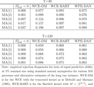
In the first part of the experiment, we study the size properties when standard asymp-totics and limit normality is used. In Table 1, we report results for various consistent estimates of σ, for T = 40 and T = 120, respectively, using limit normal asymptotics. In column WCE-DM we report the empirical size when the Diebold and Mariano WCE in (3) is used; in WCE-BART we use (5)–(6) andM =T1/3; in WPE-DAN we use the WPE estimate (10) withm =T1/2. In all these cases, as the estimates are consistent, we use standard normal limit distributions to compute the empirical size. Finally, in columnbσ2
DM <0 we report the frequency of negative estimates of the long run variance
when using the Diebold and Mariano WCE estimate as in (3).
Consistently with results in Clarks (1999), we find that, as the forecast horizon q
increases, the size of the test with the Diebold and Mariano WCE estimate deteriorates, although the size distortion is less serious in the larger sample. We also find that the risk of a negative estimate σb2
DM is not negligible, especially for small T and large q.
In comparison, using the Bartlett kernel in the WCE gives better size properties even when asymptotic normality is used, especially for the longest forecast horizons. We also experimented with the automatic bandwidth selection procedure for the Bartlett kernel in Newey and West (1994) but, as we found that this resulted in worse size properties than setting M = T1/3, in the interest of brevity we do not include it in this discussion. On balance, within the estimates that we considered, Table 1 shows that when asymptotic normality is maintained the best properties in size are for the WPE with Daniell kernel andm =T1/2, although a certain size distortion still occurs, especially in the smallest sample.
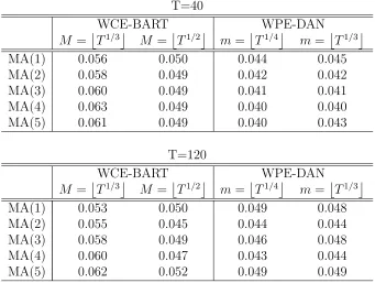
In Table 2 we report results when the properties of the estimates of σ are derived assuming fixed-b or fixed-m asymptotics. In columns WCE-BART, M = T1/3 or
Table 1: Size of tests with standard asymptotics
T=40
b
σ2
DM <0 WCE-DM WCE-BART WPE-DAN
MA(1) 0.000 0.077 0.085 0.075
MA(2) 0.001 0.099 0.090 0.076
MA(3) 0.007 0.124 0.096 0.078
MA(4) 0.017 0.157 0.097 0.081
MA(5) 0.037 0.196 0.097 0.080
T=120
b
σ2
DM <0 WCE-DM WCE-BART WPE-DAN
MA(1) 0.000 0.059 0.068 0.061
MA(2) 0.000 0.058 0.066 0.060
MA(3) 0.000 0.068 0.072 0.062
MA(4) 0.000 0.074 0.075 0.062
MA(5) 0.001 0.086 0.075 0.065
Note: empirical rejection frequencies for tests of equal predictive ability at 5% nominal size using standard normal asymptotics for various MA processes and alternative estimates of the long run variance: WCE-DM is for the WCE with the truncated kernel as in Diebold and Mariano (1995), WCE-BART is for the Bartlett kernel with M = T1/3
, and WPE-DAN for the WPE with Daniell kernel and m = T1/2
. The columnbσ2
DM <0 reports the frequency of negative estimates of the long
Table 2: Size of tests with fixed-b and fixed-m asymptotics T=40
WCE-BART WPE-DAN
M =T1/3 M =T1/2 m=T1/4 m =T1/3
MA(1) 0.056 0.050 0.044 0.045
MA(2) 0.058 0.049 0.042 0.042
MA(3) 0.060 0.049 0.041 0.041
MA(4) 0.063 0.049 0.040 0.040
MA(5) 0.061 0.049 0.040 0.043
T=120
WCE-BART WPE-DAN
M =T1/3 M =T1/2 m=T1/4 m =T1/3
MA(1) 0.053 0.050 0.049 0.048
MA(2) 0.055 0.045 0.044 0.044
MA(3) 0.058 0.049 0.046 0.048
MA(4) 0.060 0.047 0.043 0.044
MA(5) 0.062 0.052 0.049 0.049
Note: empirical rejection frequencies for tests of equal predictive ability at 5% nominal size using fixed-b or fixed-m asymptotics for various MA processes and alternative estimates of the long run variance: WCE-BART is for the WCE with Bartlett kernel withM =T1/3
orM =T1/2
WCE with Bartlett kernel and M =T1/3. The difference in size in the two tables is then due only to the different critical values. Results in Table 2 show that predictive accuracy tests with fixed-b and fixed-m asymptotics are overall correctly sized, although a slight size distortion is still present when the smaller bandwidth,M =T1/3, is used with fixed-b asymptotics.
3.2
Power Analysis
In the second part of the Monte Carlo exercise, we study the power of the proposed tests of equal predictive accuracy. In this case, we test H0 : {µ= 0} in processes with
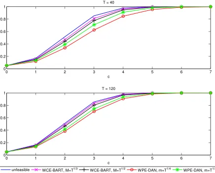
µ=cT−1/2, forcranging between 0 and 7. As in this part of the exercise we are interested in power, rather than in size distortion, we use a time series of independent, standard normal distributed variates. As in the previous exercise, we use 10000 repetitions and
T = 40 andT = 120. We compare the tests with fixed-b or fixed-m asymptotics against a benchmark case in which σ is known. With samples as small as the ones used in our experiment, this benchmark is unfeasible. If a very large sample is available, this situation can be interpreted as a limit case of the test when a WCE with b → 0 or a WPE withm→ ∞are used, so that the replacement ofσ2 with its estimate is negligible and asymptotic normality is justified. Thus, in our experiment this benchmark should be the upper bound for the empirical power functions.
The simulated empirical power is in Figure 1. Previous simulations in Kiefer and Vogelsang (2005) and in Hualde and Iacone (2015) found that the power is higher the lower is M or the larger is m, and our results are consistent with them. The test with statistic with known σ has the highest power, as expected: it is worth noting, however, that the power loss due to estimatingσ is minimal, especially when the WCE is used.
4
Predictive Accuracy of the SPF
To illustrate the usefulness of alternative asymptotics for equal predictive accuracy tests, we evaluate the predictive accuracy of the SPF forecasts for output growth, output inflation, the unemployment rate and the three-month Treasury bill rate against a simple random walk.
Figure 1: Finite sample local power
0 1 2 3 4 5 6 7
0 0.2 0.4 0.6 0.8 1
c T = 40
0 1 2 3 4 5 6 7
0 0.2 0.4 0.6 0.8 1
c T = 120
unfeasible WCE-BART, M=T1/3 WCE-BART, M=T1/2 WPE-DAN, m=T1/4 WPE-DAN, m=T1/3
The figure displays empirical rejection frequencies at 5% nominal size for deviations from the null by cT−1/2
and independent innovations. Unfeasible refers to the case in which the unknown variance is used and the test statistic has standard normal limit distribution. For the feasible tests, fixed-b or fixed-m asymptotics are used. The alternative estimates of the long run variance are: WCE-BART is for the WCE with Bartlett kernel with M =T1/3
or M = T1/2
; WPE-DAN for the WPE with Daniell kernel andm=T1/4
orm=T1/3
forecasts is the middle of the quarter. We focus on median responses for the period from 1985:Q1 until 2014:Q4 and use a quadratic loss function to evaluate the predictive accuracy of the SPF on the full sample and also on three 10-year subsamples, i.e. from 1985:Q1 to 1994:Q4, from 1995:Q1 to 2004:Q4 and from 2004:Q1 to 2014:Q4.
In the SPF, the output price index is the implicit price deflator for GNP in surveys conducted prior to 1992:Q1, the implicit deflator for GDP in the surveys from 1992:Q1 to 1995:Q4, and the chain-weighted price index in the surveys thereafter. Accordingly, real output is defined as fixed-weighted real GNP in the surveys conducted before 1992:Q1, fixed-weighted real GDP in the surveys from 1992:Q1 to 1995:Q4, and chain-weighted real GDP in the surveys thereafter. Real GNP/GDP growth and GNP/GDP inflation are constructed as the annualized quarter over quarter growth rates. For both vari-ables, we define the corresponding benchmark forecasts and realized values similarly, see Stark (2010). Finally, the three-month Treasury bill rate and the unemployment rate are expressed in levels.
We compute benchmark forecasts and realised values using the vintages of data that were available to the public before the survey’s mid-quarter deadline. For all the variables considered, we use as benchmark a naive random walk, i.e. a no change benchmark. In particular, for GNP/GDP inflation, the unemployment rate and the three-month Trea-sury bill rate, we use as benchmark a random walk on the variable. For real GNP/GDP growth, we use as benchmark a random walk with drift on real GNP/GDP levels: this is a more appropriate benchmark for real GNP/GDP growth, see Stark (2010). We estimate the drift parameter using a rolling average of real GNP/GDP growth with a window of 60 observations.
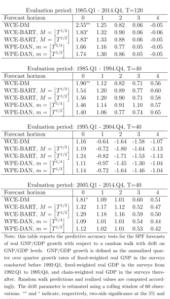
Tables 3–6 report the test statistics presented in Section 2 for the null hypothesis of equal predictive accuracy of the SPF’ forecasts for real GNP/GDP growth, GNP/GDP inflation, the unemployment rate and the three-month T-Bill rates with respect to the random walk. Results in Tables 3–6 show that the predictive ability of the SPF is stronger for the three months Treasury bill rate and GNP/GDP inflation than for real GNP/GDP growth and the unemployment rate. The subsample 1985.Q1 to 1994.Q4 is characterised by a strong predictive ability of the SPF with respect to the random walk, but this predictive ability sharply declined in the most recent subsample.
Table 3: Real GNP/GDP Growth: SPF vs. Random Walk in level
Evaluation period: 1985.Q1 - 2014.Q4, T=120
Forecast horizon 0 1 2 3 4
WCE-DM 2.55∗∗ 1.25 0.82 0.06 -0.05
WCE-BART, M =T1/3 1.83∗ 1.32 0.90 0.06 -0.06
WCE-BART, M =T1/2 1.83∗ 1.33 0.88 0.06 -0.05
WPE-DAN, m=T1/4 1.66 1.16 0.77 0.05 -0.05 WPE-DAN, m=T1/3 1.74 1.30 0.86 0.05 -0.05
Evaluation period: 1985.Q1 - 1994.Q4, T=40
Forecast horizon 0 1 2 3 4
WCE-DM 1.96∗∗ 1.12 0.82 0.71 0.56
WCE-BART, M =T1/3 1.54 1.20 0.89 0.77 0.60 WCE-BART, M =T1/2 1.56 1.20 0.90 0.71 0.58 WPE-DAN, m=T1/4 1.46 1.14 0.91 1.10 0.57 WPE-DAN, m=T1/3 1.40 1.06 0.77 0.74 0.65
Evaluation period: 1995.Q1 - 2004.Q4, T=40
Forecast horizon 0 1 2 3 4
WCE-DM 1.16 -0.64 -1.64 -1.58 -1.07
WCE-BART, M =T1/3 1.19 -0.72 -1.80 -1.64 -1.13 WCE-BART, M =T1/2 1.24 -0.82 -1.71 -1.53 -1.13 WPE-DAN, m=T1/4 1.11 -0.97 -1.45 -1.30 -1.04 WPE-DAN, m=T1/3 1.14 -0.72 -1.64 -1.46 -1.04
Evaluation period: 2005.Q1 - 2014.Q4, T=40
Forecast horizon 0 1 2 3 4
WCE-DM 1.81∗ 1.09 1.01 0.60 0.51
WCE-BART, M =T1/3 1.32 1.17 1.12 0.52 0.47 WCE-BART, M =T1/2 1.29 1.18 1.16 0.59 0.50 WPE-DAN, m=T1/4 1.09 1.01 1.01 0.54 0.44 WPE-DAN, m=T1/3 1.12 1.02 1.01 0.53 0.42
Note: this table reports the predictive accuracy tests for the SPF forecasts of real GNP/GDP growth with respect to a random walk with drift on GNP/GDP levels. GNP/GDP growth is defined as the annualized quar-ter over quarquar-ter growth rates of fixed-weighted real GNP in the surveys conducted before 1992:Q1, fixed-weighted real GDP in the surveys from 1992:Q1 to 1995:Q4, and chain-weighted real GDP in the surveys there-after. Random walk predictions and realized values are computed accord-ingly. The drift parameter is estimated using a rolling window of 60 obser-vations. ∗∗ and∗indicate, respectively, two-side significance at the 5% and
Table 4: GNP/GDP Inflation: SPF vs. Random Walk
Evaluation period: 1985.Q1 - 2014.Q4, T=120
Forecast horizon 0 1 2 3 4
WCE-DM 4.20∗∗ 3.89∗∗ 2.27∗∗ 0.73 1.67∗
WCE-BART,M =T1/3 3.28∗∗ 3.65∗∗ 2.39∗∗ 0.72 1.59 WCE-BART,M =T1/2 2.89∗∗ 3.71∗∗ 2.38∗∗ 0.62 1.57
WPE-DAN, m=T1/4 2.59∗∗ 3.23∗∗ 1.81 0.50 1.24
WPE-DAN, m=T1/3 2.69∗∗ 3.53∗∗ 2.07∗ 0.55 1.37
Evaluation period: 1985.Q1 - 1994.Q4, T=40
Forecast horizon 0 1 2 3 4
WCE-DM 2.55∗∗ 3.08∗∗ 1.45 -0.66 0.38
WCE-BART,M =T1/3 2.73∗∗ 3.09∗∗ 1.50 -0.52 0.35
WCE-BART,M =T1/2 3.08∗∗ 3.11∗∗ 1.54 -0.50 0.35
WPE-DAN, m=T1/4 3.59∗∗ 2.61∗ 1.82 -0.42 0.28
WPE-DAN, m=T1/3 4.10∗∗ 2.63∗∗ 1.38 -0.45 0.30
Evaluation period: 1995.Q1 - 2004.Q4, T=40
Forecast horizon 0 1 2 3 4
WCE-DM 1.20 1.17 0.56 0.29 0.32
WCE-BART,M =T1/3 1.04 1.19 0.59 0.33 0.38 WCE-BART,M =T1/2 0.94 1.16 0.56 0.31 0.36
WPE-DAN, m=T1/4 1.01 1.16 0.50 0.28 0.33
WPE-DAN, m=T1/3 1.04 1.21 0.54 0.30 0.31
Evaluation period: 2005.Q1 - 2014.Q4, T=40
Forecast horizon 0 1 2 3 4
WCE-DM 3.27∗∗ 2.62∗∗ 1.89∗ 1.44 4.84∗∗
WCE-BART,M =T1/3 2.42∗∗ 2.37∗∗ 2.04∗ 1.42 2.25∗∗
WCE-BART,M =T1/2 2.35∗ 2.63∗∗ 2.05∗ 1.27 2.89∗∗
WPE-DAN, m=T1/4 1.85 2.59∗ 1.91 0.99 3.07∗∗
WPE-DAN, m=T1/3 2.07∗ 2.25∗ 1.70 1.20 2.97∗∗
Note: this table reports the predictive accuracy tests for the SPF forecasts of GNP/GDP inflation with respect to a random walk. GNP/GDP inflation is defined as the implicit price deflator for GNP in surveys conducted prior to 1992:Q1, the implicit deflator for GDP in the surveys from 1992:Q1 to 1995:Q4, and the chain-weighted price index in the surveys thereafter. Random walk predictions and realized values are computed accordingly. ∗∗
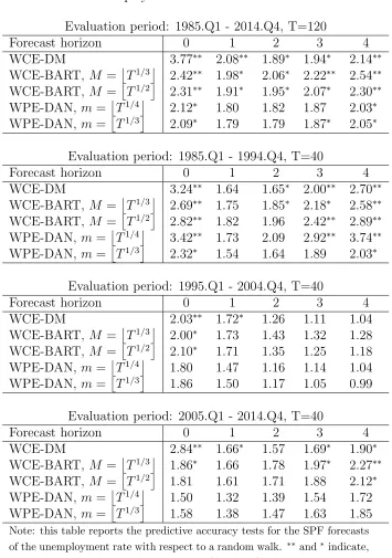
Table 5: Unemployment Rate: SPF vs. Random Walk
Evaluation period: 1985.Q1 - 2014.Q4, T=120
Forecast horizon 0 1 2 3 4
WCE-DM 3.77∗∗ 2.08∗∗ 1.89∗ 1.94∗ 2.14∗∗
WCE-BART, M =T1/3 2.42∗∗ 1.98∗ 2.06∗ 2.22∗∗ 2.54∗∗
WCE-BART, M =T1/2 2.31∗∗ 1.91∗ 1.95∗ 2.07∗ 2.30∗∗
WPE-DAN, m=T1/4 2.12∗ 1.80 1.82 1.87 2.03∗
WPE-DAN, m=T1/3 2.09∗ 1.79 1.79 1.87∗ 2.05∗
Evaluation period: 1985.Q1 - 1994.Q4, T=40
Forecast horizon 0 1 2 3 4
WCE-DM 3.24∗∗ 1.64 1.65∗ 2.00∗∗ 2.70∗∗
WCE-BART, M =T1/3 2.69∗∗ 1.75 1.85∗ 2.18∗ 2.58∗∗
WCE-BART, M =T1/2 2.82∗∗ 1.82 1.96 2.42∗∗ 2.89∗∗
WPE-DAN, m=T1/4 3.42∗∗ 1.73 2.09 2.92∗∗ 3.74∗∗
WPE-DAN, m=T1/3 2.32∗ 1.54 1.64 1.89 2.03∗
Evaluation period: 1995.Q1 - 2004.Q4, T=40
Forecast horizon 0 1 2 3 4
WCE-DM 2.03∗∗ 1.72∗ 1.26 1.11 1.04
WCE-BART, M =T1/3 2.00∗ 1.73 1.43 1.32 1.28
WCE-BART, M =T1/2 2.10∗ 1.71 1.35 1.25 1.18
WPE-DAN, m=T1/4 1.80 1.47 1.16 1.14 1.04
WPE-DAN, m=T1/3 1.86 1.50 1.17 1.05 0.99
Evaluation period: 2005.Q1 - 2014.Q4, T=40
Forecast horizon 0 1 2 3 4
WCE-DM 2.84∗∗ 1.66∗ 1.57 1.69∗ 1.90∗
WCE-BART, M =T1/3 1.86∗ 1.66 1.78 1.97∗ 2.27∗∗
WCE-BART, M =T1/2 1.81 1.61 1.71 1.88 2.12∗
WPE-DAN, m=T1/4 1.50 1.32 1.39 1.54 1.72
WPE-DAN, m=T1/3 1.58 1.38 1.47 1.63 1.85
Note: this table reports the predictive accuracy tests for the SPF forecasts of the unemployment rate with respect to a random walk. ∗∗ and∗indicate,
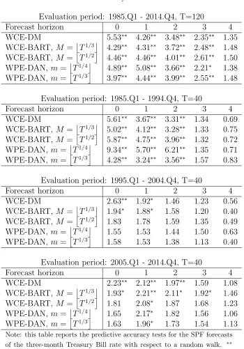
Table 6: Three-month Treasury Bill: SPF vs. Random Walk
Evaluation period: 1985.Q1 - 2014.Q4, T=120
Forecast horizon 0 1 2 3 4
WCE-DM 5.53∗∗ 4.26∗∗ 3.48∗∗ 2.35∗∗ 1.35
WCE-BART,M =T1/3 4.29∗∗ 4.31∗∗ 3.72∗∗ 2.48∗∗ 1.48
WCE-BART,M =T1/2 4.46∗∗ 4.46∗∗ 4.01∗∗ 2.61∗∗ 1.50
WPE-DAN, m=T1/4 4.89∗∗ 5.08∗∗ 3.66∗∗ 2.21∗ 1.38
WPE-DAN, m=T1/3 3.97∗∗ 4.44∗∗ 3.99∗∗ 2.55∗∗ 1.48
Evaluation period: 1985.Q1 - 1994.Q4, T=40
Forecast horizon 0 1 2 3 4
WCE-DM 5.61∗∗ 3.67∗∗ 3.31∗∗ 1.34 0.69
WCE-BART,M =T1/3 5.02∗∗ 4.12∗∗ 3.28∗∗ 1.33 0.75
WCE-BART,M =T1/2 5.87∗∗ 4.75∗∗ 3.96∗∗ 1.32 0.72
WPE-DAN, m=T1/4 9.34∗∗ 5.70∗∗ 6.21∗∗ 1.35 0.71
WPE-DAN, m=T1/3 4.28∗∗ 3.24∗∗ 3.56∗∗ 1.57 0.83
Evaluation period: 1995.Q1 - 2004.Q4, T=40
Forecast horizon 0 1 2 3 4
WCE-DM 2.63∗∗ 1.92∗ 1.46 1.23 0.56
WCE-BART,M =T1/3 1.94∗ 1.88∗ 1.58 1.20 0.40
WCE-BART,M =T1/2 1.83 1.78 1.59 1.35 0.49
WPE-DAN, m=T1/4 1.55 1.53 1.44 1.50 0.63
WPE-DAN, m=T1/3 1.58 1.53 1.38 1.13 0.40
Evaluation period: 2005.Q1 - 2014.Q4, T=40
Forecast horizon 0 1 2 3 4
WCE-DM 2.23∗∗ 2.12∗∗ 1.97∗∗ 1.59 1.08
WCE-BART,M =T1/3 1.93∗ 2.21∗∗ 2.11∗ 1.92∗ 1.46
WCE-BART,M =T1/2 1.81 2.08∗ 1.87 1.68 1.23
WPE-DAN, m=T1/4 1.65 2.17∗ 1.82 1.56 1.06
WPE-DAN, m=T1/3 1.63 1.96∗ 1.73 1.54 1.13
Note: this table reports the predictive accuracy tests for the SPF forecasts of the three-month Treasury Bill rate with respect to a random walk. ∗∗
predictive ability of the SPF, especially for short horizons and in the first and the last subsamples. Results in Table 5 indicate some predictive ability of the SPF’s forecasts for the unemployment rate, but the evidence is much weaker when using the proposed tests with fixed-b and fixed-m asymptotics. Finally, Table 6 provides strong evidence of superior predictive accuracy of the SPF’s forecasts for the three month Treasury bill rate with respect the random walk, especially for short horizons. However, the predictive ability of the SPF for the three month Treasury bill rate sharply declined in the last two subsamples.
As for the comparison of the three tests described in Section 2, we can see that the Diebold and Mariano (1995) test in (4) rejects the null hypothesis of equal predictive ability more often that the WCE and the WPE tests, especially in the subsamples. This is due to the fact that in the subsamples the tests are performed only on 40 observations, exacerbating the size distortions of the Diebold and Mariano (1995) test, see Table 1. For example, Table 5 shows that for inflation the Diebold and Mariano (1995) test rejects the null of equal predictive ability of the SPF and the random walk on the last subsample and for almost all forecasting horizons. This could be interpreted as a clear indication of predictive ability of the SPF for the unemployment rate. However, the WPE based tests fail to reject the null of equal predictive ability for all forecasting horizons, indicating that the SPF did not have any predictive ability for the unemployment rate in this period.
5
Conclusion
6
Appendix
Let xt = µ+ut, with ut = P∞l=0Alεt−l where εt is an independent, identically
dis-tributed process with E(εt) = 0, E(εt2) = 1, E(ε4t) < ∞, and
P∞
l=0j1/2|Al| < ∞. Define the Fourier frequencies λj = 0, ±1, ...,⌊T /2⌋ and the Fourier transform wx(λ) =
1
√
2πT PT
t=1xteiλt, the periodogram Ix(λ) = |wx(λ)| 2
, the sample mean x = T1 PTt=1xt
and the statistic τ = x−µ0 √
2π1
m
Pm j=1Ix(λj)
; then, under H0 :{µ=µ0}, as T → ∞,
τ →dt2m (12)
Proof. First, note that, for j = 1, ..., m, √1 2πT
PT
t=1eiλjt = 0, so wx(λj) = wu(λj). Moreover, following Hannan (1970), page 247,
wu(λ) =
X∞
l=0Ale
iλlw
ε(λ) +rT (λ)
where rT (λ) =op(1) uniformly inλ, so
wu(λj) =
X∞
l=0Ale
iλjl
wε(λj) +op(1) (13)
Now let
s2t,T = 1 2πT T X t=1 cos2 2πjt T
ηt,T =
1 √
2πTεtcos
2πjt T
zt,T = s−t,T1ηt,T
then sufficient conditions for the central limit theorem are that
E(zt,T) = 0 ∀t, T T
X
t=1
V (zt,T) = 1 ∀t, T
zt,T independent from zs,T ∀t, s, ∀T T
X
t=1
E|zt,T|2+δ →0 for someδ >0
verified for δ = 1, noting that E|εt|3 exists becauseE(ε4t)<∞. Thus,
T X
t=1
zt,T →dN(0,1)
i.e., 1 2πT T X t=1 cos2 2πjt T
!−1/2 T
X
t=1 1 √
2πTεtcos
2πjt T
→ dN(0,1)
T X
t=1 1 √
2πTεtcos
2πjt T
→ dN
0, 1
2π1/2
where we also used T1
T P t=1
cos2 2πjt T
= 12 from Gradshteyn and Ryzhik (1994), equation
(1.351.2), page 37, and conclude
1/2 1 2π
−1 XT
t=1 1 √
2πTηtcos
2πjt T
!2
→dχ21
The term √1
2πT T P t=1
εtsin 2πjtT
may be discussed in the same way. The covariance of
T P t=1
1
√
2πTεtcos
2πjt T
and PT
t=1 1
√
2πTεtsin
2πjt T is 1 2πT T X t=1 sin 2πjt T cos 2πjt T = 0
using Gradshteyn and Ryzhik (1994), equation (1.333.1), page 35, and then equation
(1.342.1), page 36. Then, the joint convergence of
T P t=1
1
√
2πTεtcos
2πjt T and T P t=1 1 √
2πTεtsin
2πjt T
to a bivariate vector of independently distributed random variables with diagonal co-variance matrix follows from an application of the Cramer-Wold device.
Therefore,
2 (2π)Iε(λj)→d χ22.
Moreover, as in Hannan (1970), page 249,
and therefore
2π 1 m
Xm
j=1Iε(λj)→d C 2
2m/(2m)
whereC2
2m/(2m) is a χ22m distributed random variable divided by the number of degrees
of freedom.
Using (13) and P∞l=0Aleiλjl →P∞l=0Al =σ, it also follows that
2π 1 m
Xm
j=1Ix(λj)→dσ 2C2
2m/(2m) .
Finally, proceeding as in Phillips and Solo (1992), we use the Beveridge Nelson decom-position
ut=
X∞
l=0Al
εt+εet−1−εet
where
e
εt=
X∞
l=0Aelεt−l, Ael =
X∞
k=l+1Ak
and
1 √
T
XT
t=1ut=
X∞
l=0Al
1
√
T
XT
t=1εt+ 1 √
T (εe0−εeT) (14)
where √1
T (eε0−εeT) = op(1) as in Phillips and Solo (1992) page 978. In view of Remark
3.5 of Phillips and Solo (1992), the condition on the weights Al is P∞l=0Ae2l < ∞, as
in equation (16) of Phillips and Solo (1992), and this is implied by P∞l=0l1/2|A
l|< ∞,
Phillips and Solo (1992) page 973, so
1 √
T
XT
t=1ut=σ 1 √
T
XT
t=1εt+op(1)→dN 0, σ 2.
Finally, it is easy to verify that
E 1 √ Tσ XT
t=1εt
X∞
l=0Ale
iλjlw
ε(λj)
= σ
P∞
l=0Aleiλjl
√
2πT E
XT
t=1εt
XT
s=1εse
iλjs
= σ
P∞
l=0Aleiλjl
√ 2πT
XT
s=1e
iλjs = 0
and thus conclude that (12) holds.
Remark. ConditionP∞l=0l1/2|A
l|<0 is fairly common in the literature, and it holds
7
References
Clark, T.E., 1999. Finite-sample properties of tests for equal forecast accuracy,Journal of Forecasting, 18, 489-504.
Clark, T. E., and McCracken, M. W., 2001. Tests of Equal Forecast Accuracy and Encompassing for Nested Models, Journal of Forecasting , 105, 85-110.
Clark, T. E., and McCracken, M. W., 2013, Advances in Forecast Evaluation, in Hand-book of Economic Forecasting (Vol. 2), eds. G. Elliott and A. Timmerman, Amsterdam: Elsevier, 1107-1201.
Diebold, F.X., 2015. Comparing Predictive Accuracy, Twenty Years Later: A Personal Perspective on the Use and Abuse of Diebold-Mariano Tests, Journal of Business and Economic Statistics, 33:1, 1-9.
Diebold, F.X., and R.S. Mariano, 1995. Comparing predictive accuracy, Journal of Business and Economic Statistics, 20, 134-144.
Giacomini, R., and Rossi, B., 2010. Forecast Comparisons in Unstable Environments,
Journal of Applied Econometrics, 25, 595-620.
Gradshteyn, I.S., and I.M. Ryzhik, 1994. Table of Integrals, Series, and Products, Fifth Edition. Academic Press, Boston.
Hannan, E.J., 1970. Multiple time series, Wiley, New York.
Harvey, D., S.J. Leybourne, P. Newbold, 1997. Testing the equality of prediction mean squared errors, International Journal of Forecasting, 13, 281-291.
Hualde, J., and F. Iacone, 2015. Autocorrelation robust inference using the Daniell ker-nel with fixed bandwidth, Discussion Papers in Economics No. 15/14, Department of Economics, University of York.
Kiefer, N.M., and T.J. Vogelsang, 2005. A new asymptotic theory for heteroskedasticity-autocorrelation robust tests, Econometric Theory , 21, 1130-1164.
Kokoszka, P., and T. Mikosch, 2000. The periodogram at the Fourier frequencies,
Stochastic Processes and their Applications, 86, 49–79.
M¨uller, U. K., 2014. HAC Corrections for Strongly Autocorrelated Time Series,Journal of Business & Economic Statistics, 32:3, 311-322.
Newey, W. K. and K. D. West, 1994. Automatic lag selection in covariance matrix estimation, Review of Economic Studies, 61, 631-653.
Patton, A. J., 2015. Comment, Journal of Business and Economic Statistics, 33:1, 22-24.
Phillips, P. C. B., and V. Solo, 1992. Asymptotics for linear processes, Annals of Statistics, 20, 971-1001.
Stark, T., 2010. Realistic evaluation of real-time forecasts in the survey of professional forecasters. Research Rap Special Report, Federal Reserve Bank of Philadelphia.