From KIDSCREEN-10 to CHU9D: creating a unique mapping algorithm for application in economic evaluation

R E S E A R C H

Open Access

From KIDSCREEN-10 to CHU9D: creating a unique

mapping algorithm for application in economic

evaluation

Gang Chen

, Katherine Stevens

, Donna Rowen

and Julie Ratcliffe

Abstract

Background:The KIDSCREEN-10 index and the Child Health Utility 9D (CHU9D) are two recently developed generic instruments for the measurement of health-related quality of life in children and adolescents. Whilst the CHU9D is a preference based instrument developed specifically for application in cost-utility analyses, the KIDSCREEN-10 is not currently suitable for application in this context. This paper provides an algorithm for mapping the KIDSCREEN-10 index onto the CHU9D utility scores.

Methods:A sample of 590 Australian adolescents (aged 11–17) completed both the KIDSCREEN-10 and the CHU9D. Several econometric models were estimated, including ordinary least squares estimator, censored least absolute deviations estimator, robust MM-estimator and generalised linear model, using a range of explanatory variables with KIDSCREEN-10 items scores as key predictors. The predictive performance of each model was judged using mean absolute error (MAE) and root mean squared error (RMSE).

Results:The MM-estimator with stepwise-selected KIDSCREEN-10 items scores as explanatory variables had the best predictive accuracy using MAE, whilst the equivalent ordinary least squares model had the best predictive accuracy using RMSE.

Conclusions:The preferred mapping algorithm (i.e. the MM-estimate with stepwise selected KIDSCREEN-10 item scores as the predictors) can be used to predict CHU9D utility from KIDSCREEN-10 index with a high degree of accuracy. The algorithm may be usefully applied within cost-utility analyses to generate cost per quality adjusted life year estimates where KIDSCREEN-10 data only are available.

Keywords:Health-related quality of life, CHU9D, KIDSCREEN, Mapping, Utility, Adolescent

Background

Health-related quality of life (HRQoL) is a multidimen-sional construct that measures the impact of health or disease on physical and psychosocial functioning [1,2]. The measurement and valuation of HRQoL is a major issue for health services research and has become an es-sential component for assessing the cost-effectiveness of treatments and interventions in public health and clical medicine research internationally [3]. HRQoL in-struments can be categorised into two groups: health

profile measures providing simple summative index sum-mary scores for individual dimensions (items) and/or over-all health, and preference based instruments/multi-attribute utility instruments containing preference weights for indi-vidual dimensions relative to each other and a preference weighted summary score for each health state defined by the instrument. Multi-attribute utility instruments can be used to generate quality adjusted life years (QALYs) for use in cost-utility analyses. QALYs are the preferred outcome measure for many regulatory bodies including the National Institute for Health and Clinical Excellence in the UK and the Pharmaceutical Benefits Advisory Committee in Australia [3,4].

The majority of HRQoL instruments developed specific-ally for children and adolescent populations are not * Correspondence:[email protected]

1

Flinders Health Economics Group, School of Medicine, Flinders University, Adelaide, Australia

3

A Block, Level 1, Repatriation General Hospital, School of Medicine, Flinders University, Daws Road, Daw Park, SA 5041, Australia

Full list of author information is available at the end of the article

suitable for application within the framework of cost-utility analysis because they are non-preference based. One of the most prevalent non-preference based instru-ments, widely used in both public health and clinical medicine disciplines across countries, is the KIDSCREEN [5-8]. The KIDSCREEN has a simple summative scoring system in which equal weights are attached to different di-mensions of HRQoL. However, a valid instrument that can be used to generate QALYs in cost-utility analyses needs to have the ability to ‘measure’ health status and also the ability to ‘value’ health status by incorporating preferences relating to the relative desirability of the di-mensions and severity levels of each of the didi-mensions in-cluded in the instrument.

Mapping or cross walking techniques may be applied to link profile instruments and preference based instru-ments together thereby enabling non-preference based HRQoL instrument results to be utilised within the framework of cost-utility analyses [4,9]. A comprehen-sive review by Brazier and colleagues [9] identified 30 mapping studies in the literature. All of these studies had been conducted using instruments designed for measuring HRQoL in adults, and had been applied exclusively in adult populations. To date, only one previous study has conducted a mapping exercise exclusively in a paediatric population. Furber and colleagues mapped the Strengths and Difficulties Questionnaire responses into Child Health Utility 9D (CHU9D) utilities [10].

The main objective of this study was to develop an al-gorithm for generating CHU9D utility scores from KIDSCREEN-10 index summary scores, facilitating cost-utility analyses within studies where health outcomes are assessed only by the KIDSCREEN-10 index.

Methods Study design

An online survey was developed for administration to a community based sample of adolescents living in

Australia, aged 11–17 years. Following parent and

ado-lescent consent, adoado-lescents were invited to complete a survey which included the CHU9D and KIDSCREEN-10 instruments, socio-demographic variables (gender, age and socio-economic status as measured by the Family Affluence Scale) [11], a five-scale self-reported general health question (measured as excellent, very good, good, fair and poor), and whether they had a long standing disability, illness or medical condition. This study was approved by the Social and Behavioural Research Ethics Committee, Flinders University (project number 4701).

Instruments

The KIDSCREEN-10 is a generic non-preference based measure of well-being and HRQoL developed inter-nationally for children and adolescents aged 8 to 18 years

old [5]. It is a short version of the KIDSCREEN-52 and KIDSCREEN-27 instruments and has demonstrated cri-terion validity, convergent validity and known groups validity [12,13]. The KIDSCREEN-10 contains 10 items: fit and well (KS_I1), energy (KS_I2), sad (KS_I3), lonely (KS_I4), had enough time for yourself (KS_I5), been able to do the things that you want to do in your free time (KS_I6), parent(s) treated you fairly (KS_I7), had fun with friends (KS_I8), got on well at school (KS_I9) and been able to pay attention (KS_I10), each with a 5 point response scale [13]. The calculation of KIDSCREEN-10 index involve three steps: firstly, a raw overall score is summed by adding each item score with equal weight; secondly, the sum scores are converted to a score by assigning Rasch person parameters to each possible sum score; and lastly, the person parameters are transformed into values with a mean of approximately 50 and standard deviation approximately 10 [12]. A higher score is indica-tive of a better HRQoL. Both self-reported and parent proxy versions are available for KIDSCREEN instruments. The self-reported version was adopted in this study.

The CHU9D is a newly developed generic preference based measure of HRQoL that was designed specifically for application with young people [14]. Whilst it was ori-ginally developed for use with younger children aged 7 to 11 years, recent studies have also demonstrated the practi-cality and validity of using CHU9D in older adolescent

populations aged 11–17 years [15-17]. The CHU9D

con-sists of 9 dimensions: worried, sad, pain, tired, annoyed, schoolwork/homework, sleep, daily routine, ability to join in activities, with 5 different levels representing increasing levels of severity within each dimension. The original health state valuation algorithm for CHU9D was gener-ated from the application of the standard gamble method within the UK adult general population [18]. In this study, since Australian adolescent data is used, we applied a re-cently developed Australian adolescent specific scoring algorithm for the CHU9D instrument based upon the

best-worst scaling method and anchored on the 1–0

full-health to dead scale using the UK standard gamble results [19]. The CHU9D utilities range between 0.33 and 1. The strength of overlap between the KIDSCREEN-10 and the CHU9D has been reported in detail elsewhere [17]. Briefly Stevens and Ratcliffe found a moderate degree of signifi-cant correlation between CHU9D utility scores and the KIDSCREEN-10 index (r = 0.61), with some differences in the coverage of the items for the respective descriptive sys-tems. The KIDSCREEN-10 is broader in scope than the CHU9D which focuses on a narrower definition of HRQoL.

Statistical analysis

used to estimate the mapping algorithm that can then be applied to other studies. In this study two groups of models were considered. In the first group the CHU9D utility score was regressed upon the KIDSCREEN-10 index, and also a higher order of the KIDSCREEN-10 index if the relation-ship between the two instruments was found to be non-linear. In the second group the CHU9D utility score was regressed upon the individual KIDSCREEN-10 item raw re-sponse scores. In the event that not all KIDSCREEN-10 items coefficients were statistically significant, the stepwise regression with forward selection technique (with signifi-cance levels for entrance of 0.05) was used to choose the “best”combination of predictors from the 10 items [20]. In the mapping literature, Model 2 is the most widely used additive model [9]. In addition to individual item and over-all summary scores several previous mapping studies have also included socio-demographic characteristics, in particu-lar age and gender, to improve predictive performance [9]. The significance (or otherwise) of including age and gender was also considered here. To summarise, the following two models were considered.

CHU9D¼αþβ1⋅KSþβ2þKS2þδ1⋅Ageþδ2⋅Gender(Model 1)

CHU9D¼αþXk_j¼1γj⋅KSIjswþδ1⋅Ageþδ2⋅Gender(Model 2)

where CHU9D is the CHU9D utility score, KS is the

KIDSCREEN-10 index, KS2is the KIDSCREEN-10 index

squared, KS_Ij_sw are the selected KIDSCREEN-10 items based upon statistical significances using the step-wise regression technique, k is the number of selected KIDSCREEN-10 items. The significance level is set to be 5% in this study.

Several econometric techniques have been adopted in previous studies to estimate mapping models, of which the ordinary least squares estimator has been the most widely adopted [9,21]. The majority of mapping models in the lit-erature have mapped to EQ-5D, and as a result models are used that are appropriate for the distribution of EQ-5D re-sponses which is typically bi-modal or tri-modal with a large proportion of responses at 1 (see Longworth and Rowen [22] for an overview). Figure 1 indicates that for this sample CHU9D responses are left-skewed with a large number of responses at 1. Appropriate estimators include: the Tobit estimator which takes into account bounding is-sues (e.g. for some multi-attribute utility instruments a high proportion of respondents report full health with a utility of 1), the censored least absolute deviations estimator which further relaxes the distributional assumption of the error term (i.e. not necessarily requiring the error term to be normal and homoscedastic as assumed by Tobit) [23,24], and the generalised linear model which allows for the non-normal distribution of dependent variables (e.g. left/negatively skewed utility scores) [25].

The ordinary least squares estimator is sensitive to potential outliers as it is based on the minimisation of

the variance of the residuals. The censored least absolute deviations estimator mentioned above is a special case of robust regressions that does not suffer from this sen-sitivity and is therefore considered to be more suitable in this context. In this study we propose to include an-other effective robust estimator, the MM-estimator [26], that has been shown to have both a high breakdown point (i.e. the percentage of incorrect observations an es-timator can handle before giving an incorrect result) and a high efficiency [27,28], but has not yet been utilised in mapping exercises. Heteroskedasticity robust standard errors are reported for inference.

Previous studies have indicated that the censored least absolute deviations estimator outperforms the Tobit esti-mator in relation to goodness-of-fit criteria (e.g. mean pre-diction error) (see for example Sullivan and Ghushchyan [29]). However since no other definitive evidence is avail-able regarding the superiority of a particular estimator, we chose to utilise four estimators (ordinary least squares, censored least absolute deviations, MM and generalised linear model) in this study. Among different combinations

of family and link function for the generalised linear

model, the binomial family with logit link was chosen as the most appropriate since it showed the best performance of predicting the mean utility close to the observed. Re-gression analyses were estimated in Stata version 12.1 (StataCorp LP, College Station, Texas, USA).

Goodness-of-fit was examined using mean absolute

error (MAE) and root mean square error (RMSE) –

whereby the lower the value, the better the perform-ance. MAE was selected as the key criteria to measure average model performance as it has been found to be a more natural measure of average error than RMSE; it is unambiguous [30].

generated through the full sample were tested on three random samples [33]. The three random samples with sample size of 100, 300, and 500 were generated by ran-dom selection within the full sample.

Results

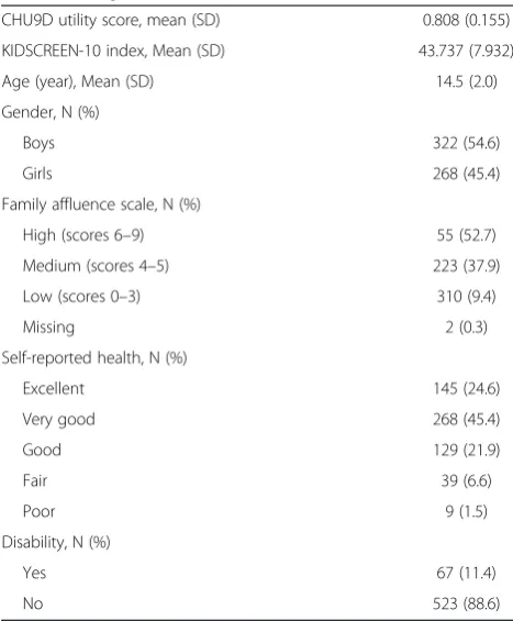
Of the 961 adolescents who consented to take part in the survey, 590 adolescents (61.4%) completed both the CHU9D and KIDSCREEN-10 instruments and had no missing values on age and gender. The mean (standard deviation) CHU9D utility score was 0.808 (0.155) and mean (standard deviation) KIDSCREEN-10 index was 43.737 (7.932). Fifty five percent of respondents were male, the mean (standard deviation) age was 14.5 (2) years, 53% of respondents came from families with high socio-economic status (as defined by the Family Afflu-ence Scale), 92% reported their health status was good, very good or excellent, 11% had a disability. See Table 1 for details.

Figure 1 shows the kernel density of the CHU9D util-ity scores and the KIDSCREEN-10 index. The CHU9D utility score is non-normally (left-skewed) distributed while the KIDSCREEN-10 index tends towards a normally distribution (although the null hypothesis for normality was rejected based on Shapiro-Wilk normality test).

Pairwise Pearson’s correlations between each item of the KIDSCREEN-10 index and CHU9D utility score suggest that the strongest correlated item is KS_I1 (“fit and well”, r = 0.488), followed by another 5 items with a correlation higher than 0.4, i.e. KS_I10 (r = 0.447), KS_I3 (r = 0.437), KS_I2 (r = 0.427), KS_I4 (r = 0.416) and KS_I9 (r = 0.406). The remaining 4 items have a correlation with a CHU9D utility score that is lower than 0.4, including KS_I5 (r =

0.365), KS_I8 (r = 0.317), KS_I7 (r = 0.271) and the lowest

correlated item was KS_I6 (“been able to do the things

that you want to do in your free time”, r = 0.175).

Prediction of CHU9D utility scores

The goodness-of-fit results for different combinations of models and methods of the full sample are reported in

Table 1 Sample characteristics

CHU9D utility score, mean (SD) 0.808 (0.155)

KIDSCREEN-10 index, Mean (SD) 43.737 (7.932)

Age (year), Mean (SD) 14.5 (2.0)

Gender, N (%)

Boys 322 (54.6)

Girls 268 (45.4)

Family affluence scale, N (%)

High (scores 6–9) 55 (52.7)

Medium (scores 4–5) 223 (37.9)

Low (scores 0–3) 310 (9.4)

Missing 2 (0.3)

Self-reported health, N (%)

Excellent 145 (24.6)

Very good 268 (45.4)

Good 129 (21.9)

Fair 39 (6.6)

Poor 9 (1.5)

Disability, N (%)

Yes 67 (11.4)

No 523 (88.6)

CHU9D - Child Health Utility 9D; SD - standard deviation.

0

1

2

3

4

5

.2 .4 .6 .8 1

CHU9D utility score (best-worst scaling method)

0

.02

.04

.06

.08

Density

20 40 60 80

KIDSCREEN-10 index

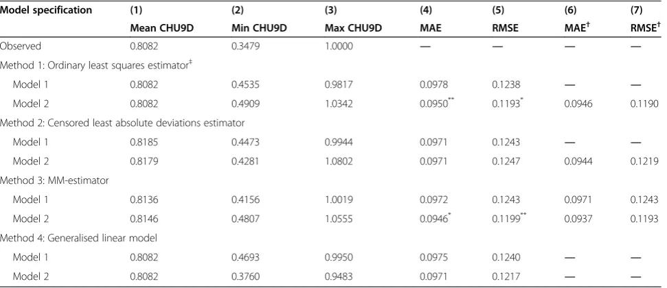
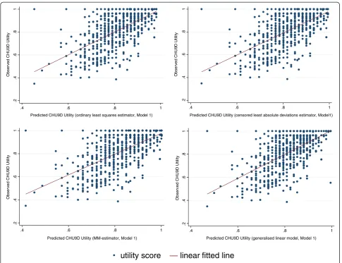
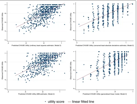
Table 2. All estimators tend to over predict the lowest boundary of the utility score and among them, the general-ised linear model estimate, based on Model 2, is closest to the observed score (0.3760 vs. 0.3479, Column 2). On the highest boundary of the utility score, estimators may either over or under-estimate the maximum utility. According to the absolute difference, the MM-estimate, based on Model 1, performs the best (1.0019 vs. 1, Column 3). For the two goodness-of-fit indicators, the MM-estimate has the lowest MAE (0.0946, Column 4) and the second lowest RMSE (0.1199, Column 5), whilst the ordinary least squares esti-mate has the lowest RMSE (0.1193, Column 5) and the sec-ond lowest MAE (0.0950, Column 4). Based on the results presented in Table 2, it is reasonable to conclude that the mapping algorithm using the MM-estimator with model 2 specification is preferred based on MAE criteria. Scatter-grams of the relationship between the observed and the KIDSCREEN-10 predicted CHU9D utility scores are shown in the Figures 2 and 3.

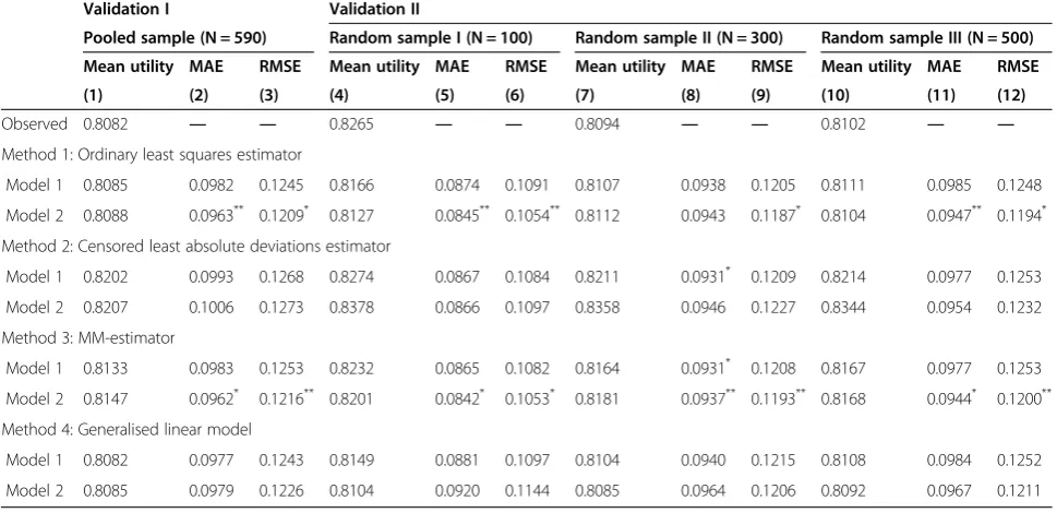
Validation

Table 3 reports two groups of validation analyses results for all combinations of models and methods introduced in the statistical analysis section. According to MAE and RMSE, ordinary least squares and MM-estimates based on the model 2 specification have the best predictive per-formance across both methods of valuation. Overall the MM-estimates based on the model 2 specification are se-lected as the preferred model as it performs slightly better using the preferred MAE criteria. The results reported in validation analyses support the conclusion from the full

sample analysis that MM-estimator based on Model 2 is the optimal choice if MAE is the key criteria, whilst the ordinary least squares estimator based on Model 2 should be chosen if RMSE is the dominant one.

Mapping equations

The detailed regression results using the full sample are reported in Table 4. Gender was consistently insignifi-cant in all scenarios. Age was found to be signifiinsignifi-cant only one occasion where the ordinary least squares esti-mator was applied. For all other three estiesti-mators, age was insignificant. Considering these findings, both gen-der and age were not included in the final regression equa-tions. For Model 1, both the original KIDSCREEN-10 index and its squared term were found to be robustly significant (P < 0.05) in three estimates (ordinary least squares, cen-sored least absolute deviations and MM-estimator), indicat-ing the existence of the non-linear relationship between the two instruments. The generalised linear model incorporates the nonlinear relationship between dependent and inde-pendent variables through the link function, and as shown in Model 1, the coefficient of the KIDSCREEN-10 index was statistically significant (P < 0.05) whilst the squared term was insignificant and not included.

In Model 2, the stepwise selected significant KIDSCREEN-10 items are the key predictors. As can be seen, not all of the 10 items were significant, but for all statistically significant items the positive coefficients were consist-ent with the expectation that a high item score (better health) is associated with a higher utility. The potential multicollinearity issue was detected using variance

Table 2 Goodness-of-fit results from full sample

Model specification (1) (2) (3) (4) (5) (6) (7)

Mean CHU9D Min CHU9D Max CHU9D MAE RMSE MAE† RMSE†

Observed 0.8082 0.3479 1.0000 ― ― ― ―

Method 1: Ordinary least squares estimator‡

Model 1 0.8082 0.4535 0.9817 0.0978 0.1238 ― ―

Model 2 0.8082 0.4909 1.0342 0.0950** 0.1193* 0.0946 0.1190

Method 2: Censored least absolute deviations estimator

Model 1 0.8185 0.4473 0.9944 0.0971 0.1243 ― ―

Model 2 0.8179 0.4281 1.0802 0.0971 0.1247 0.0944 0.1219

Method 3: MM-estimator

Model 1 0.8136 0.4156 1.0019 0.0972 0.1243 0.0971 0.1243

Model 2 0.8146 0.4807 1.0555 0.0946* 0.1199** 0.0937 0.1193

Method 4: Generalised linear model

Model 1 0.8082 0.4693 0.9950 0.0975 0.1240 ― ―

Model 2 0.8082 0.3760 0.9483 0.0971 0.1217 ― ―

CHU9D–Child Health Utility 9D; MAE–mean absolute error; RMSE–root mean squared error. *denotes the smallest value in the column; **denotes the second smallest value in the column.

inflation factor and the mean/highest variance inflation factor in this case is 1.88/2.01, suggestion that none of the items suffered from multicollinearity and can be in-cluded simultaneously in the regressions. The items that were found to be robustly non-significant across four estimators were KS_I5 (“had enough time for yourself”),

KS_I6 (“been able to do the things that you want to do

in your free time”), KS_I7 (“parent(s) treated you fairly”) and KS_I8 (“had fun with friends”). This is consistent with the findings from the pairwise correlation analysis, specific-ally that all four items exhibited a relative lower correlation relationship with CHU9D (r < 0.4). A bootstrap stepwise or-dinary least squares regression technique (with 100 replica-tions) was also conducted. Ranked by the number of times each variable is selected, KS_I3 topped the list (100 out of 100 times been selected), followed by KS_I1 (99 out of 100), KS_I10 (93 out of 100), KS_I4 (91 out of 100), KS_I9 (59 out of 100), KS_I2 (55 out of 100), KS_I7 (36 out of 100), KS_I8 (29 out of 100), KS_I5 (21 out of 100), and KS_I6 (8 out of 100). Consistent with these findings, KS_I7, KS_I8, KS_I5, and KS_I6 demonstrate the least importance

in mapping onto the CHU9D utility. See Table 4 for the de-tailed regression outputs of four estimators. Based on the MAE result discussed above, the optimal equation used to predict the CHU9D utility based on KIDSCREEN-10 items would be:

CHU9D utility score = 0.222655 + 0.037867*KS_I1 + 0.023085*KS_I2 + 0.037192*KS_I3 + 0.021284*KS_I4 + 0.024877*KS_I9 + 0.022256*KS_I10.

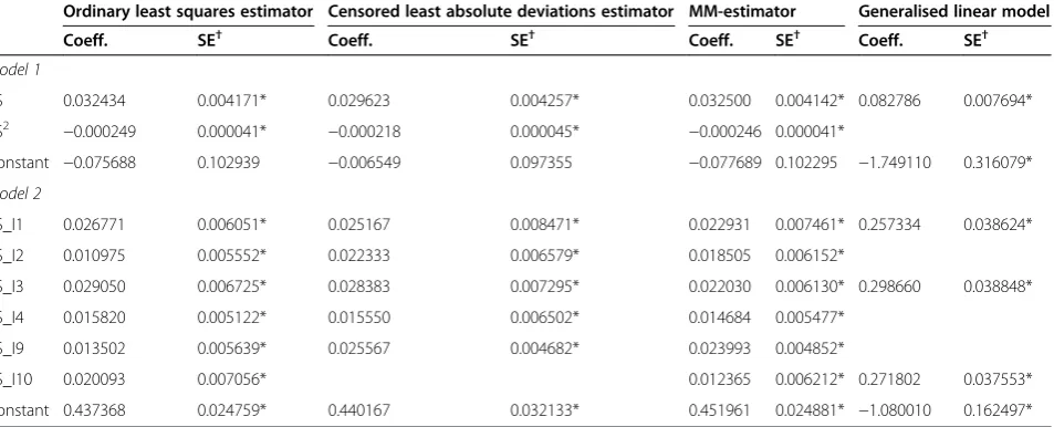
As previously highlighted, there are currently two preference based scoring algorithms available for the CHU9D, the original one generated by the standard gamble method with the UK adult general population and a newly developed one generated by the best-worst scaling method with the Australian adolescent general

population and anchored on the 1–0 full health-dead

scale using the UK values. The utility scores generated by application of the two scoring algorithms are highly correlated (r = 0.97). The correlation between each item of the KIDSCREEN-10 instrument and each of the two util-ity scores are almost identical. Owing to word limits, the analyses presented here were based upon the Australian

.2

.4

.6

.8

1

.4 .6 .8 1

Predicted CHU9D Utility (ordinary least squares estimator, Model 1)

Observed CHU9D Utility

.2

.4

.6

.8

1

.4 .6 .8 1

Predicted CHU9D Utility (censored least absolute deviations estimator, Model1)

Observed CHU9D Utility

.2

.4

.6

.8

1

.4 .6 .8 1

Predicted CHU9D Utility (MM-estimator, Model 1)

Observed CHU9D Utility

.2

.4

.6

.8

1

.4 .6 .8 1

Predicted CHU9D Utility (generalised linear model, Model 1)

Observed CHU9D Utility

utility score

—

linear fitted line

adolescent general population scoring algorithm. The key mapping equations (corresponding to those reported in Table 4) from the KIDSCREEN-10 index to the CHU9D utility scores based upon the UK adult scoring algorithm are also reported in the Table 5 for the readers’ interest. The goodness-of-fit results also suggest that the ordinary least squares and MM-estimates based on the Model 2 spe-cification had the best predictive performance, and the MM-estimates based on the Model 2 specification is se-lected as the preferred model using MAE.

Discussion

The measurement and valuation of the HRQoL of chil-dren and adolescents is increasingly being recognised as an important component of economic evaluations of health care treatment and preventive programs targeted for young people. The KIDSCREEN-10 instrument has been validated across several European countries for the measurement of health status and since its development in 2004 the instrument has been also widely used across coun-tries. However, a current limitation of the KIDSCREEN-10

is the absence of preference weights meaning that the measure cannot be used directly to estimate QALYs for use in cost-utility analyses. This study has developed a mapping algorithm that can be used to predict CHU9D utility scores based on the KIDSCREEN-10 index. The utilisation of the algorithm will enable cost-utility analyses to be conducted within studies where health outcomes were assessed using only the KIDSCREEN-10 index.

There are two main strengths of this study. Firstly, the target and base measures are both generic HRQoL in-struments and as such they have a conceptual overlap between each other. This is an important determinant to the success of mapping analysis [9,22,34]. Secondly, mul-tiple estimators that are appropriate for the data have been adopted to explore the optimal mapping algorithms [22]. Specifically, we have used the MM-estimator, an effective robust estimator to map the KIDSCREEN-10 to CHU9D. The MM-estimator has not to our knowledge been previ-ously used in mapping and in this dataset outperforms the censored least absolute deviations and generalised linear model techniques that have been used previously in the

.2

.4

.6

.8

1

.4 .6 .8 1

Predicted CHU9D Utility (ordinary least squares estimator, Model 2)

Observed CHU9D Utility

.2

.4

.6

.8

1

.4 .6 .8 1

Predicted CHU9D Utility (censored least absolute deviations estimator, Model 2)

Observed CHU9D Utility

.2

.4

.6

.8

1

.4 .6 .8 1

Predicted CHU9D Utility (MM-estimator, Model 2)

Observed CHU9D Utility

.2

.4

.6

.8

1

.4 .6 .8 1

Predicted CHU9D Utility (generalised linear model, Model 2)

Observed CHU9D Utility

utility score

linear fitted line

mapping literature, and performs similarly to ordinary least squares in this dataset. As the MM-estimator offers some theoretical advantages over ordinary least squares estimator and performs similarly for this reason it is our preferred model here. The model performance as indicated by MAE (0.0946) of the preferred MM-estimate model based on the Model 2 specification is within the range reported by previ-ously published studies (0.0011 to 0.19) [9].

Despite our preference for the MM-estimator, it should be noted that these two estimators do perform similarly. In terms of their predictive ability as the

RMSE value (0.1193) of the optimal ordinary least squares estimate is also within the published ranges (0.084 to 0.2) [9]. The largely comparable predictive performance of ordinary least squares and MM-estimator models, des-pite the MM-estimator overcoming the theoretical limita-tions of ordinary least squares estimator for the analysis of CHU9D, is of interest. However in the literature this has also been found in some studies mapping onto the EQ-5D using ordinary least squares estimator and other models overcoming the theoretical limitations of ordinary least squares estimator [22].

Table 3 Goodness-of-fit results from validation analysis

Validation I Validation II

Pooled sample (N = 590) Random sample I (N = 100) Random sample II (N = 300) Random sample III (N = 500)

Mean utility MAE RMSE Mean utility MAE RMSE Mean utility MAE RMSE Mean utility MAE RMSE

(1) (2) (3) (4) (5) (6) (7) (8) (9) (10) (11) (12)

Observed 0.8082 ― ― 0.8265 ― ― 0.8094 ― ― 0.8102 ― ―

Method 1: Ordinary least squares estimator

Model 1 0.8085 0.0982 0.1245 0.8166 0.0874 0.1091 0.8107 0.0938 0.1205 0.8111 0.0985 0.1248

Model 2 0.8088 0.0963** 0.1209* 0.8127 0.0845** 0.1054** 0.8112 0.0943 0.1187* 0.8104 0.0947** 0.1194*

Method 2: Censored least absolute deviations estimator

Model 1 0.8202 0.0993 0.1268 0.8274 0.0867 0.1084 0.8211 0.0931* 0.1209 0.8214 0.0977 0.1253

Model 2 0.8207 0.1006 0.1273 0.8378 0.0866 0.1097 0.8358 0.0946 0.1227 0.8344 0.0954 0.1232

Method 3: MM-estimator

Model 1 0.8133 0.0983 0.1253 0.8232 0.0865 0.1082 0.8164 0.0931* 0.1208 0.8167 0.0977 0.1253

Model 2 0.8147 0.0962* 0.1216** 0.8201 0.0842* 0.1053* 0.8181 0.0937** 0.1193** 0.8168 0.0944* 0.1200**

Method 4: Generalised linear model

Model 1 0.8082 0.0977 0.1243 0.8149 0.0881 0.1097 0.8104 0.0940 0.1215 0.8108 0.0984 0.1252

Model 2 0.8085 0.0979 0.1226 0.8104 0.0920 0.1144 0.8085 0.0964 0.1206 0.8092 0.0967 0.1211

MAE–mean absolute error; RMSE–root mean squared error.

*denotes the smallest value in the column; **denotes the second smallest value in the column.

Table 4 Mapping equations from KIDSCREEN-10 index to Child Health Utility 9D utility scores

Ordinary least squares estimator Censored least absolute deviations estimator MM-estimator Generalised linear model

Coeff. SE† Coeff. SE† Coeff. SE† Coeff. SE†

Model 1

KS 0.043515 0.005291* 0.046580 0.006828* 0.049504 0.006682* 0.092650 0.008747*

KS2 _{−0.000334 0.000053* −0.000359 0.000072* −0.000384 0.000070*}

Constant −0.435412 0.129225* −0.510120 0.160989* −0.593052 0.157245* −2.472760 0.359525*

Model 2

KS_I1 0.035797 0.008005* 0.059820 0.009940* 0.037867 0.010995* 0.296834 0.042888*

KS_I2 0.017943 0.007725* 0.023085 0.009292*

KS_I3 0.037163 0.008005* 0.039315 0.011111* 0.037192 0.009329* 0.331778 0.040524*

KS_I4 0.022713 0.006543* 0.027291 0.010421* 0.021284 0.007952*

KS_I9 0.016046 0.007037* 0.024877 0.008434*

KS_I10 0.027138 0.008991* 0.060152 0.010321* 0.022256 0.010361* 0.300356 0.041449*

Constant 0.250215 0.029866* 0.156848 0.053203* 0.222655 0.034914* −1.735730 0.167557*

†_{Heteroskedasticity robust standard errors (SE). *significant at 5%. For generalised linear model,binomialfamily andlogitlink were used.}

Although aggregated sample/group level and dis-aggregated individual level predictions of CHU9D utility scores can be incorporated within economic evaluation, it is recommended that only the aggregated sample/ group level prediction be adopted based on the current al-gorithm. At the individual level the predicted utility scores are less reliable as the prediction error could be large as indicated in the Figures 2 and 3. The over-prediction at the lower end of utility values is an issue that not uncommon in the mapping analysis where re-gression technique is used [35]. Furthermore, as can be seen from Columns (2) and (3) of Table 2, there is no guarantee that the predicted utility will lie within the observed ranges if the transformation algorithm is based upon ordinary least squares estimator, censored least absolute deviations or MM- estimators. Some studies have suggested that in practice if the predicted utility fell outside the defined range, then it should be truncated to the appropriate boundary value (e.g. Sullivan

and Ghushchyan [29], Wu et al. [31], Payakachat et al.

[36]). Following this suggestion, the predicted utility score should be specified to 1 if the prediction is larger than 1. How this modification will change the goodness-of-fit re-sults in our sample is shown in Columns (6) and (7) of Table 2. As can be seen, this adjustment always improves the goodness-of-fit results.

This study has some limitations. Response rates and data quality are two potential issues with online modes of survey administration. On-line modes of administra-tion are increasingly familiar, particularly for young people and have the potential to engage large numbers of com-munity based adolescents who would otherwise be more

difficult to reach. It is possible to include checks for data quality in on-line surveys and we have taken care to scru-tinise the data generated for illogical responses and to check that respondents appeared to understand the task adequately. It is also important to note that other modes of survey administration including self-completion ques-tionnaires and interviews may also be plagued by low re-sponse rates and issues of data quality.

In relation to the modelling approach adopted it is im-portant to highlight that model performance was vali-dated using the internal dataset only. A cross-validation would be ideal once a suitable external dataset becomes available. In addition, the study sample was relatively healthy and as such it is also possible that the best per-forming model specification and type would have dif-fered if the mapping algorithms had been estimated using a dataset with a larger number of respondents in poorer health. Therefore, an external validation using a patient sample is recommended prior to using these mapping algorithms in a dataset with children in poor health. An alternative mapping method, the linking ap-proach that has not yet been empirically tested could be explored in future studies [37].

Conclusion

When a preference based instrument has not been in-cluded in a study to enable QALYs to be estimated for use in cost-utility analyses, the adoption of a mapping approach from a non-preference based instrument to obtain health state utilities served as a second best alterna-tive facilitating cost-utility analyses. This paper has pro-duced a mapping algorithm to generate a CHU9D utility

Table 5 Mapping equations from KIDSCREEN-10 index to UK Child Health Utility 9D utility scores

Ordinary least squares estimator Censored least absolute deviations estimator MM-estimator Generalised linear model

Coeff. SE† Coeff. SE† Coeff. SE† Coeff. SE†

Model 1

KS 0.032434 0.004171* 0.029623 0.004257* 0.032500 0.004142* 0.082786 0.007694*

KS2

−0.000249 0.000041* ₋0.000218 0.000045* ₋0.000246 0.000041*

Constant ₋0.075688 0.102939 ₋0.006549 0.097355 ₋0.077689 0.102295 ₋1.749110 0.316079*

Model 2

KS_I1 0.026771 0.006051* 0.025167 0.008471* 0.022931 0.007461* 0.257334 0.038624*

KS_I2 0.010975 0.005552* 0.022333 0.006579* 0.018505 0.006152*

KS_I3 0.029050 0.006725* 0.028383 0.007295* 0.022030 0.006130* 0.298660 0.038848*

KS_I4 0.015820 0.005122* 0.015550 0.006502* 0.014684 0.005477*

KS_I9 0.013502 0.005639* 0.025567 0.004682* 0.023993 0.004852*

KS_I10 0.020093 0.007056* 0.012365 0.006212* 0.271802 0.037553*

Constant 0.437368 0.024759* 0.440167 0.032133* 0.451961 0.024881* −1.080010 0.162497*

Note: Predicted utility values are for the UK scoring algorithm of the Child Health Utility 9D based on adult values elicited using standard gamble.

†_{Heteroskedasticity robust standard errors. *significant at 5%. For generalised linear model,binomialfamily andlogitlink were used.}

score from KIDSCREEN-10 items. The preferred model is the MM-estimate with stepwise selected KIDSCREEN-10 item scores as the predictors (i.e. Model 2 in Table 4) ac-cording to the MAE. The ordinary least squares estimate with stepwise selected KIDSCREEN-10 item scores as the predictors also show good performance based on RMSE.

Competing interests

The authors declare that they have no competing interests.

Authors_’contributions

GC carried out the data analyses and drafted the manuscript. KS and DR critically revised the manuscript. JR supervised the project, collected the data and critically revised the manuscript. All authors read and approved the final manuscript.

Acknowledgements

This paper has benefited from presentation at the 9th World Congress of the International Health Economics Association (iHEA). We are grateful to Dr. Billingsley Kaambwa from Flinders University and three anonymous referees for their detailed and helpful comments. Responsibility for any remaining errors or omissions lies solely with the authors.

Financial support

Financial support from a Flinders University seeding grant and an Australian NHMRC Project Grant 1021899 entitled_‘Adolescent values for the economic evaluation of adolescent health care treatment and preventive programs’is gratefully acknowledged.

Author details

1

Flinders Health Economics Group, School of Medicine, Flinders University, Adelaide, Australia.2_{Health Economics and Decision Science, School of} Health and Related Research, University of Sheffield, Sheffield, UK.3A Block, Level 1, Repatriation General Hospital, School of Medicine, Flinders University, Daws Road, Daw Park, SA 5041, Australia.

Received: 25 March 2014 Accepted: 14 August 2014 Published: 29 August 2014

References

1. Fontaine K, Barofsky I:Obesity and health-related quality of life.Obes Rev 2001,2(3):173–182.

2. Tsiros M, Olds T, Buckley J, Grimshaw P, Brennan L, Walkley J, Hills AP, Howe PR, Coates AM:Health-related quality of life in obese children and adolescents.Int J Obes2009,33(4):387–400.

3. Brazier JE, Ratcliffe J, Tsuchiya A, Salomon J:Measuring and Valuing Health Benefits for Economic Evaluation.New York: Oxford University Press; 2007. 4. National Institute for Health and Care Excellence:Guide to the methods of

technology appraisal 2013. http://www.nice.org.uk/article/PMG9/chapter/ Foreword.

5. Erhart M, Ottova V, Gaspar T, Jericek H, Schnohr C, Alikasifoglu M, Morgan A, Ravens-Sieberer U, HBSC Positive Health Focus Group:Measuring mental health and well-being of school-children in 15 European countries using the KIDSCREEN-10 Index.Int J Public Health2009,54(Suppl 2):160–166. 6. Crespo C, Carona C, Silva N, Canavarro M, Dattilio F:Understanding the quality of life for parents and their children who have asthma: family resources and challenges.Contemp Fam Ther2011,33(2):179–196. 7. Levin KA:Glasgow smiles better: an examination of adolescent mental

well-being and the‘Glasgow effect’.Public Health2012,126(2):96–103. 8. Block K, Gibbs L, Staiger PK, Gold L, Johnson B, Macfarlane S, Long C,

Townsend M:Growing community: the impact of the Stephanie Alexander Kitchen Garden Program on the social and learning environment in primary schools.Health Educ Behav2012,39(4):419–432. 9. Brazier JE, Yang Y, Tsuchiya A, Rowen DL:A review of studies mapping

(or cross walking) non-preference based measures of health to generic preference-based measures.Eur J Health Econ2010,11(2):215–225. 10. Furber G, Segal L, Leach M, Cocks J:Mapping scores from the Strengths

and Difficulties Questionnaire (SDQ) to preference-based utility values. Qual Life Res2014,23(2):403–411.

11. Boyce W, Torsheim T, Currie C, Zambon A:The Family Affluence Scale as a measure of national wealth: validation of an adolescent self-report measure.Soc Indic Res2006,78(3):473–487.

12. Ravens-Sieberer U, The KIDSCREEN Group Europe:The KIDSCREEN Questionnaires—Quality of Life Questionnaires for Children and Adolescents— Handbook.Lengerich: Pabst Science Publisher; 2006.

13. Ravens-Sieberer U, Erhart M, Rajmil L, Herdman M, Auquier P, Bruil J, Power M, Duer W, Abel T, Czemy L, Mazur J, Czimbalmos A, Tountas Y, Hagquist C, Kilroe J, European KIDSCREEN Group:Reliability, construct and criterion validity of the KIDSCREEN-10 score: a short measure for children and adolescents_’ well-being and health-related quality of life.Qual Life Res2010,19(10):1487–1500. 14. Stevens K:Developing a descriptive system for a new preference-based

measure of health-related quality of life for children.Qual Life Res2009, 18(8):1105–1113.

15. Ratcliffe J, Couzner L, Flynn T, Sawyer M, Stevens K, Brazier J, Burgess L: Valuing Child Health Utility 9D health states with a young adolescent sample: a feasibility study to compare best-worst scaling discrete-choice experiment, standard gamble and time trade-off methods.Appl Health Econ Health Policy2011,9(1):15–27.

16. Ratcliffe J, Stevens K, Flynn T, Brazier J, Sawyer M:An assessment of the construct validity of the CHU9D in the Australian adolescent general population.Qual Life Res2012,21(4):717–725.

17. Stevens K, Ratcliffe J:Measuring and valuing health benefits for economic evaluation in adolescence: an assessment of the practicality and validity of the Child Health Utility 9D in the Australian adolescent population. Value Health2012,15(8):1092–1099.

18. Stevens K:Valuation of the child health utility 9D index.Pharmacoeconomics 2012,30(8):729_–747.

19. Ratcliffe J, Flynn T, Terlich F, Stevens K, Brazier J, Sawyer M:Developing adolescent-specific health state values for economic evaluation: an application of profile case best-worst scaling to the Child Health Utility 9D.Pharmacoeconomics2012,30(8):713–727.

20. Rabe-Hesketh S, Everitt B:A Handbook of Statistical Analyses Using Stata (Fourth Edition).Boca Raton, FL: Chapman & Hall/CRC; 2007. 21. Mortimer D, Segal L:Comparing the incomparable? A systematic

review of competing techniques for converting descriptive measures of health status into QALY-weights.Med Decis Mak2008, 28(1):66–89.

22. Longworth L, Rowen D:The use of mapping to obtain EQ-5D utility values for use in NICE health technology assessments.Value Health2013, 16(1):202_–210.

23. Jolliffe D, Krushelnytskyy B, Semykina A:Censored least absolute deviations estimator: CLAD.Stata Tech Bull2006,58:13–16.

24. Cameron AC, Trivedi PK:Microeconometrics: Methods and Applications.New York: Cambridge University Press; 2005.

25. Fox J:Applied Regression Analysis and Generalized Linear Models (Second Edition).Thousand Oaks, CA: SAGE Publications; 2008.

26. Yohai VJ:High breakdown-point and high efficiency robust estimates for regression.Ann Stat1987,15(2):642–656.

27. Verardi V, Croux C:Robust regression in Stata.Stata J2009,9(3):439–453. 28. Jann B:ROBREG: Stata module providing robust regression estimators.

http://ideas.repec.org/c/boc/bocode/s457114.html.

29. Sullivan P, Ghushchyan V:Mapping the EQ-5D index from the SF-12: US general population preferences in a nationally representative sample. Med Decis Mak2006,26(4):401–409.

30. Willmott CJ, Matsuura K:Advantages of the mean absolute error (MAE) over the root mean square error (RMSE) in assessing average model performance.Clim Res2005,30(1):79–82.

31. Wu EQ, Mulani P, Farrell MH, Sleep D:Mapping FACT-P and EORTC QLQ-C30 to patient health status measured by EQ-5D in metastatic hormone-refractory prostate cancer patients.Value Health2007, 10(5):408_–414.

32. Wong CKH, Lam CLK, Rowen D, McGhee SM, Ma K-P, Law W-L, Poon JT, Chan P, Kwong DL, Tsang J:Mapping the functional assessment of cancer therapy-general or -colorectal to SF-6D in Chinese patients with colorectal neoplasm.Value Health2012,15(3):495–503.

33. Kontodimopoulos N, Aletras V, Paliouras D, Niakas D:Mapping the cancer-specific EORTC QLQ-C30 to the preference-based EQ-5 D, SF-6 D, and 15 D instruments.Value Health2009,8:1151–1157.

35. Rowen D, Brazier J, Roberts J:Mapping SF-36 onto the EQ-5D index: how reliable is the relationship?Health Qual Life Outcomes2009,7(1):27. 36. Payakachat N, Summers K, Pleil A, Murawski M, Thomas J III, Jennings K,

Anderson JG:Predicting EQ-5D utility scores from the 25-item National Eye Institute Vision Function Questionnaire (NEI-VFQ 25) in patients with age-related macular degeneration.Qual Life Res2009,18(7):801–813. 37. Fayers PM, Hays RD:Should linking replace regression when mapping

from profile-based measures to preference-based measures?Value Health 2014,17(2):261–265.

doi:10.1186/s12955-014-0134-z

Cite this article as:Chenet al.:From KIDSCREEN-10 to CHU9D: creating a unique mapping algorithm for application in economic evaluation.

Health and Quality of Life Outcomes201412:134.

Submit your next manuscript to BioMed Central and take full advantage of:

• Convenient online submission

• Thorough peer review

• No space constraints or color figure charges

• Immediate publication on acceptance

• Inclusion in PubMed, CAS, Scopus and Google Scholar

• Research which is freely available for redistribution