Real-time diffuse optical tomography using reduced-order light propagation models based on a priori anatomical and functional information

This is a repository copy of

Real-time diffuse optical tomography using reduced-order light

propagation models based on a priori anatomical and functional information

.

White Rose Research Online URL for this paper:

http://eprints.whiterose.ac.uk/74671/

Monograph:

Vidal-Rosas, E.E., Coca, D., Billings, S.A. et al. (4 more authors) (2010) Real-time diffuse

optical tomography using reduced-order light propagation models based on a priori

anatomical and functional information. Research Report. ACSE Research Report no. 1020

. Automatic Control and Systems Engineering, University of Sheffield

[email protected] https://eprints.whiterose.ac.uk/

Reuse

Unless indicated otherwise, fulltext items are protected by copyright with all rights reserved. The copyright exception in section 29 of the Copyright, Designs and Patents Act 1988 allows the making of a single copy solely for the purpose of non-commercial research or private study within the limits of fair dealing. The publisher or other rights-holder may allow further reproduction and re-use of this version - refer to the White Rose Research Online record for this item. Where records identify the publisher as the copyright holder, users can verify any specific terms of use on the publisher’s website.

Takedown

If you consider content in White Rose Research Online to be in breach of UK law, please notify us by

Real-Time Diffuse Optical Tomography Using Reduced-Order

Light Propagation Models

Based on

a priori

Anatomical and

Functional Information

Ernesto E. Vidal-Rosas

, Daniel Coca

, Stephen A. Billings

, Ying Zheng

, John E.W.

Mayhew,

David Johnston

, Aneurin Kennerly

1

Department of Automatic Control & Systems Engineering

Department of Psychology

The University of Sheffield

Department of Automatic Control and Systems Engineering

The University of Sheffield, Sheffield, S1 3JD, UK

Research Report No. 1020

REAL-TIME DIFFUSE OPTICAL TOMOGRAPHY USING REDUCED-ORDER

LIGHT PROPAGATION MODELS

BASED ON

A PRIORI

ANATOMICAL AND

FUNCTIONAL INFORMATION

Ernesto E. Vidal-Rosas1, Daniel Coca1*, Stephen A. Billings1, Ying Zheng2, John E.W. Mayhew, 2 David Johnston2, Aneurin Kennerly2

1_{Department of Automatic Control & Systems Engineering} 2_{Department of Psychology}

The University of Sheffield Mappin Street, Sheffield, S1 3JD

[email protected]

ABSTRACT

This paper proposes a new fast 3D image reconstruction algorithm for Diffuse Optical Tomography using reduced order polynomial mappings from the space of optical tissue parameters into the space of flux measurements at the detector locations. The polynomial mappings are constructed through an iterative estimation process involving structure detection, parameter estimation and cross-validation using data generated by simulating a diffusion approximation of the radiative transfer equation incorporating a priori anatomical and functional information provided by MR scans and prior psychological evidence. Numerical simulation studies demonstrate that reconstructed images are remarkably similar in quality as those obtained using the standard approach, but obtained at a fraction of the time.

KEY WORDS

Diffuse Optical Tomography, Near-infrared Imaging, Inverse Problem

1. Introduction

Diffuse Optical Tomography (DOT) is a noninvasive imaging modality that employs near-infrared light to interrogate optical properties of biological tissue [6]. Compared with alternative imaging modalities, such as functional Magnetic Resonance Imaging (fMRI), DOT has several advantages, including portability, low-cost instrumentation, fast acquisition time with the potential for real-time monitoring, and also disadvantages, particularly relatively low spatial resolution.

One way to improve the quality of the image reconstruction, is to use a priori structural information provided by an alternative imaging modality such as MRI to construct anatomically realistic 3D tissue model which are then used to solve the forward problem i.e. predict the distribution of light at the detector locations [1].

Another factor preventing routine clinical use is the considerable amount of time and computational resources

required to reconstruct a tomographic image of optical tissue properties.

For two-dimensional problems, image reconstruction is achieved relatively fast. However, most real life applications, involve the reconstruction of 3D maps of optical properties. The discretization of the 3D problem using the Finite Element Method (FEM) produces very large matrices which lead to computationally intensive reconstruction algorithms [12]. In general, the more accurate the forward model, the more computationally demanding the reconstruction algorithm. As a consequence, real-time imaging is only possible at the expense of image quality.

In this paper, a novel solution to solve the inverse problem based on a reduced-order forward model is proposed. This approximate model is a nonlinear mapping from the space of optical parameters to the space of measurements, and therefore no matrix inversion is required to solve the forward problem.

To investigate the potential of the proposed algorithms, a simulation experiment was designed consisting on the reconstruction of absorption changes due to brain activity in a realistic rat’s head derived from MRI scans.

2. Basic Theory and Algorithms

2.1 The Forward Problem

Let ⊂IR3 with boundary be the medium of interest and let u(r) be the vector of optical parameter functions (for example μa(r) and μs(r)) of the medium at position r∈

. The forward problem is defined as follows: given the sources q=[q1,…,qs] on ∂ and the optical parameters u(r)∈U, predict detector measurements { ( )}y j j=1,s

_,

given only source qj.

The forward problem is described by the following parameters-to-output mapping,

( ) _j ( ), 1,...,

where Pj:U Γ is the forward operator from the space of

parameter functions _U=_Uμa×_Uμs _{to the space of}

measurements Y= IRd, given the source qj.

The forward operator is obtained by combining a nonlinear forward map F:U , where is the space of solutions to the governing light propagation model (the forward model), with a measurement operator M: Y.

A model of light propagation through tissue, which is commonly used in applications involving Continuous Wave DOT systems [1], is the diffusion approximation of the Radiative Transfer Equation (RTE),

( )

( )

( ) ( )

( )

D r φ r μ r φ r q r r

−∇ ⋅ ∇ + = ∈Ω (2) where φj(r) is the spatially varying diffuse photon density

at position r given the source qj, µa is the absorption

coefficient, D 3

(

)

= ⎡_⎣ + ⎤_⎦ is the diffusion coefficient, and μs′ is the reduced scattering coefficient. The

collimated source incident at ξj∈ ∂Ω is usually

represented by an isotropic point source q r_j

( )

(

)

where rj is located at a depth of one scattering length

inside the medium, along the direction of the normal vector to the surface at the source location nf

( )

The boundary condition usually employed is of the Robin type

( )

( )

( )

0 2 j j D n A φ ξ

ξ ∂ + φ ξ = ξ∈∂Ω

∂ (3)

where the term A accounts for the refractive index boundary mismatch between the interior and exterior mediums.

For any given source qj, the variable measured by the

detector located at ξi∈ ∂Ω is the outward fluxγ ξj( )i .The

corresponding measurement equations are given by ( ) ( ) ( ) ( ),

( ) ( ), 1,..., ; 1,...,

j j

i j i

D n

y j

j s i d

γ ξ ξ ξ φ ξ ξ

γ ξ

= − ⋅ ∇ ∈ Ω

=

= =

f

(4).

In practice, detectors are co-located with the source optodes and the measurements are obtained using a time-multiplexed illumination scheme. Specifically, each source is activated sequentially while the remaining s-1 optodes act as detectors.

2.2 Image Reconstruction

The inverse problem is to recover the optical medium parameters given the sources q and measurements on the boundary ∂ . The output least squares formulation is given by

2

1

Minimize ( ) over

s

j _Y

j

P u y j u U U

=

− ∈ ⊂

∑

where U# is the admissible parameter space. This is an infinite dimensional optimization problem. In practice, only an approximate solution can be computed based on a sequence of finite dimensional approximating problems. In

this paper, the finite dimensional optimization problem is formulated over finite-element state and parameter spaces

N_{⊂ and U}#M _⊂U#_{respectively. The reconstruction}

algorithm is based on a finite dimensional linear perturbation equation, derived from (1),

( ) ( , ), 1,...,

M M

j

W δu t =δy j t j= s (5)

where δuM(t) is the vector of changes in the optical parameters relative to a reference medium at time t, WM is the sensitivity matrix or Jacobian, which relates changes in optical parameters corresponding to each mesh element to changes in the outward flux measured at every detector location given the source j, and δy j t( , ) is a vector of normalized differences between two sets of optode readings taken at time t given source j. Specifically, for the

i-th optode

0, 0, ( , ) ( ) ˆ ( , ) ( ) ( ) i i i i i

y j t y j

y j t y j

y j

δ = − (6)

where yi(j,t) is a measurement taken at time t, y0,i is the

time average mean and ˆ ( )y ji is the predicted

measurement corresponding to the reference medium. This type of inverse formulation is called Normalized Difference Method (NDM) [7].

The finite dimensional optimization problem (which has to be solved for every time point separately) is given by

2 1

Minimize ( ) over

s

M M M M

j _Y

j

W δu δy j δu U

=

⋅ − ∈

∑

In this paper, the above optimization problem was solved using an iterative Conjugate-Gradient (CG) algorithm [10]. This iterative approach is computationally demanding as it requires solving the diffusion equation and the recalculation of the Jacobian, at every iteration.

3. Tomographic Reconstruction Algorithm

using Reduced-order Forward Models

3.1 Polynomial Approximation of the Forward Model

The approach proposed here to speed up the reconstruction process involves constructing a reduced-order polynomial approximation of the nonlinear mapping (1) using simulated data generated by a conventional finite element approximation of the forward model given in equations (2)-(4). The FEM-based forward model is called the complete model.

The reduced-order model of (1) can be expressed in its component form as

, 1 ,

ˆ ( ) ( M,..., M) , 1,..., ;

i i j n i j

y j = f u u +e i j= s i≠ j (8) where ˆ ( )y ji is the predicted measurement at the ith

optode location computed using the forward model (2)-(4) given the source qj, fi,j is a polynomial approximation,

( )

M M

k k k

u =u r is the absorption value for the k-th node, n is the total number of nodes and ei,j is the approximation

which involves finding both the structure and the parameters of the unknown function fi,j. Model structure

detection and parameter estimation for linear-in-the- parameters polynomial models has been extensively studied and efficient algorithms are readily available [2].

3.2 Model Structure Detection and Parameter Estimation

Expansion of model (8) as a full multivariable polynomial function of a given degree l yields

1 ,

0

ˆ ( ) ( , ) ( ,..., ) L

M M

i k k M i j

k

y j θ i j p u u e

=

=

∑

where { k(i,j)} are the coefficients and pk are monomials of

degree less than or equal to l. The number of terms L in a polynomial representation grows exponentially with the number of inputs and with the order of the polynomial. In practice however, only a small number of terms are needed to represent the relationship between optical parameters and detector measurements.

Selection of a minimal model subset given the full set of candidate polynomial terms in (9) is known as a model structure detection problem. Once the correct model structure (which is linear in the parameters) is determined, the parameters can be estimated vary quickly using least-squares based algorithms. In this work, model structure detection and parameter estimation was performed using an efficient Orthogonal Forward Regression procedure, the details of which can be found in [2].

3.2 Model Validation

Model validation is required to ensure that the estimated model can be used to predict correctly detector measurements given any arbitrary combination of optical parameters within the range of interest. The approach employed here to assess the predictive ability of the regressions models is known as cross-validation [3]. Input and output data for each source detector pair comprised of 2K sets of input-output samples. The first K records were used as an estimation data set and the remaining samples as validation data. The goodness of fit for each model component was evaluated using the root mean square error (RMSE)

( )

( )

(

)

1

ˆ

, ,

RMSE( , )

K V

i i

t

y j t y j t

i j

K

=

−

=

∑

where yiV denote measurements not used to estimate the

model and yˆ the output of the model.

3.3 Model Estimation in the 2D Case

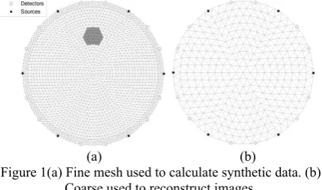
For simplicity, the procedure to estimate the reduced forward model is illustrated using a simple geometry as an example. The extension to the three-dimensional case is straightforward. Consider the circular background region shown in Figure 1a with radius r = 25mm and optical parameters μa = 0.015 mm

-1 _and

s

μ′ = 1 mm-1. The

medium was discretized using 4278 elements and 2209 nodes. Around the boundary, 6 sources and 18 detectors were located at equispaced intervals resulting in 102 source-detector pairs (no measurement was taken at the same place where a source was delivering light). This mesh was used for the simulation of measurement data.

To solve the inverse problem, a second independent mesh with lower resolution was used as the reconstruction base [11]. This mesh is shown in Figure 1b and consists of 593 elements and 325 nodes.

(a) (b)

Figure 1(a) Fine mesh used to calculate synthetic data. (b) Coarse used to reconstruct images.

To generate the data needed to estimate and validate the reduced forward model, 1000 normally distributed random absorption values were used to compute detector measurements using the FEM approximation of the forward model in equations (2)-(4). The mean value was chosen as the background absorption coefficient µa =

0.015 mm-1. The variance was chosen according to the magnitude of the expected perturbation. The maximum value of absorption coefficient for the inhomogeneity was considered to be constrained to ±10% the value of the background absorption coefficient, thus the variance was selected as 2 = 0.0015. The first 500 records were used as estimation data and remaining records as validation data. For each input u(r,t)=µa(r,t), the forward model was

simulated to generate the corresponding measurements. Assuming a second order polynomial function and 325 inputs, results in a model set of 53301 candidate monomials. However, by applying the OFR algorithm, the reduced models estimated for each source-detector pair are much smaller. For example, the reduced-order model estimated for source 2, (r, ) = (25, /3) and detector 7, (r,

) = (25, /3) has only 40 terms as shown below

2 0 1 205 254 2 159 202 3 119 203 4 157 262 5 160 208 6 210 263 7 158 161 8 204 209 9 117 207 10 162 264 11 118 156 12 163 255 13 257 261 14 120 206 15 116 253 16 121 256

17 260 (5)

y u u u u u u u u

u u u u u u u u

u u u u u u u u

u u u u u u u u

u u

θ θ θ θ θ

θ θ θ θ

θ θ θ θ

θ θ θ θ

θ

= + + + +

+ + + +

+ + + +

+ + + +

+ _{316 18 85 86 19 84 258 20 83 259}

21 201 254 22 122 211 23 155 164 24 162 317 25 82 203 26 55 58 27 56 315 28 87 261 29 115 202 30 54 57 31 123 207 32 310 314 33 34 200 34 157 308 35

u u u u u u

u u u u u u u u

u u u u u u u u

u u u u u u u u

u u u u u

θ θ θ

θ θ θ θ

θ θ θ θ

θ θ θ θ

θ θ θ

+ + +

+ + + +

+ + + +

+ + + +

+ + + 309 313 36 81 252

37 254 311 38 33 209 39 255 260

u u u

u u u u u u

θ

θ θ θ

+

+ + +

where the inputs uk= µa(rk) are identified by their finite

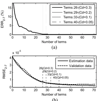
element mesh index. The terms of the model given in (11) are selected using the Error Reduction Ratio (ERR) criterion [2]. The OFR algorithm computes the ERR of each candidate term and uses this to rank the contribution of each term (Figure 2a). The algorithm stops when ERR is below a certain threshold. In this example, the cut-off value chosen was Cd =0.05. This corresponds roughly to the

point at which the RMSE error does not improve significantly by adding more terms (Figure 2b).

To illustrate the efficiency of the algorithm, the Photon Measurement Density Function (PMDF) [1], which describes the sensitivity of a source-detector pair to changes of the optical parameters inside the medium, is shown in Figure 3a for the source-detector pair 2-7. Analysis of the model (11) shows that all the coordinates of all variables uk selected in the model using the OFR

algorithm, correspond to points within the 5% ‘banana-shaped’ area shown in Figure 3a. In other words, a tolerance of 5% in the Jacobian corresponds approximately to the Cd = 0.05 ERR cut-off value, as shown in Figure3b.

Several other thresholds are displayed as contour lines in Figure 3a,b.

It is worth noting that Eames [5] found that removing regions from the Jacobian whose contribution to the measurement is approximately less than 5% can be used as an efficient method to reduce the size of the Jacobian matrix WM. These results demonstrate that there is a clear relation between the sensitivity measure provided by the Jacobian and the ERR criterion used by the model selection algorithm. An important consequence of this result is that the information provided by the PMDF function can be used to reduce the initial search space for the OFR algorithm. Effectively, the candidate model set should be constructed based only on the inputs that lie inside the region inside which PMDF>1%-5%.

3.4 Image Reconstruction Using the Reduced Forward Model

To test the reconstruction algorithm, a circular inclusion with radius R = 3 mm and 13 mm offset the centre was embedded in the medium as shown in Figure 1a. The optical parameters inside the perturbation were varied according to the following quasi-periodic function [7]

( )

cos sin

2 8 4

a t t t

π π

μ = ⎡⎢ ⎛⎜ ⎟⎞ + ⎛⎜_⎜ ⎞⎟_⎟ ⎤⎥ ⎝ ⎠

⎢ ⎝ ⎠ ⎥

⎣ ⎦ (12)

The reconstruction problem was to determine the location of the perturbation and quantify it based on simulated detector measurements.

The inverse problem was solved for each time point using the CGD algorithm limited to 1000 iterations. For comparison purposes, the inverse problem was solved using both the standard FEM-based approach and the reduced model approach.

0 10 20 30 40 50 60 70

0 5 10 15

Number of terms

ER R2 -7 (% ) Terms:26-(Cd=0.3) Terms:29-(Cd=0.2) Terms:33-(Cd=0.1) Terms:40-(Cd=0.05) (a)

0 10 20 30 40 50 60 70

0 1 2 3 4

x 10-5

26(Cd=0.3) 29(Cd=0.2)

33(Cd=0.1) 40(Cd=0.05)

Number of terms

R M S E2 -7 Estimation data Validation data (b)

Figure 2 (a) Reduction of the mean squared error as more terms are included in the model. (b) Cross-validation test

to check for overfitting.

0.05 0.3 1

(a) (b)

Figure 3. (a) Different thresholds of the Jacobian for source 2- detector 7 shown as contour lines. (b) Selected nodes at different Cd values shown as growing regions for the same

source-detector pair.

The quality of image reconstruction images was assessed using the Image Correlation Coefficient (ICC), which measures the spatial accuracy [7]:

(

)(

)

(

)

(

)

1 ( , )

1

i i

A A B B i

i i

A A B B

i i

x x x x

ICC A B

N _{x x x x}

− −

=

− _{− −}

∑

∑

∑

where i A

x , i

B

x denote the intensities of the ith pixel in images A and B respectively and xA, xB denote the mean

intensities of the two images. The correlation coefficient has a value of 1 if the images are identical, and 0 if the images are completely uncorrelated. In our case, image A corresponds to the original image and image B corresponds to the image reconstructed using either the FEM-based solver or the reduced model approach.

resolved the location of the inclusion accurately but the magnitude is not recovered. It is important to mention that as a result of the inverse formulation employed, i.e. NDM, the aim is to recover the dynamic behaviour of the inclusion and not the absolute value.

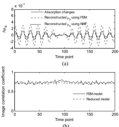
The quality of the dynamic reconstruction is illustrated in Figure 6. Figure 6a shows the original and reconstructed time varying absorption coefficient at a point located at the centre of the inclusion. Both methods fail to recover the absolute change; however the dynamic variation is easily distinguished. For each reconstructed image, the correlation coefficient defined by equation (13) was also calculated and this is displayed in Figure 6b. In general, the performance of the FEM-based approach is better than the reduced model by 3.7%, on average.

Image reconstructions were carried out using a MATLAB implementation of the algorithms on a standard PC with a single core 3GHz Intel Pentium microprocessor and 1GB RAM. Image reconstruction based on the FEM-model took ~180 seconds for each time point while for the reduced forward model it took ~40 seconds. In this case, the speed-gain is not significant. However, the advantage of using the reduced forward model will be evident in 3D reconstruction.

(a) (b)

Figure 4 Reconstruction of first sample from the tomography set using (a) FEM-based approach and (b) the

reduced model. Dashed lines indicate the location of the inclusion.

-20 -10 0 10 20

-1 0 1 2

3x 10

-3

y (mm)

Δ

μa

Original Perturbation FEM model Reduced model

Figure 5 Amplitude profiles of reconstructed absorption coefficient.

0 50 100 150 200

-4 -2 0 2 4 6 8x 10

-3

Time point

Δ

μa

Absorption changes Reconstructed μ_a using FEM Reconstructed μa using NMF

(a)

0 50 100 150 200

0 0.5 1

Time point

Im

a

g

e

c

o

rr

e

la

ti

o

n

c

o

e

ff

ic

ie

n

t

FEM model Reduced model

(b)

Figure 6 Reconstruction of the complete time series using conventional FEM-based approach (– –) and reduced model approach (- -), original signal is denoted with the

continuous line. (b) Behaviour of the correlation coefficient along the time series.

4. Fast 3D Tomographic Reconstruction using

Reduced-Order Models

4.1 FEM Forward Solver Incorporating a priori

Structural and Functional Information

It is well known that the use of a priori structural and functional information improves the DOT reconstruction significantly [6]. Structural priors usually refer to the anatomical boundaries between different tissue subdomains while functional priors typically refer to known optical properties of the heterogeneous medium. The simplest way to incorporate such information in the forward model is to use a secondary imaging modality, such as MRI, to identify the boundaries between different tissue types and, assuming that there is a high correlation between the anatomical and optical images, assign typical values for optical absorption and scattering parameters for each tissue subdomain [4]. More flexible, statistical prior models have also been proposed [8].

(a) (b) (c) Figure 7 Fine mesh generation. (a) MRI image, (b) 3D model after segmentation and (c) final tetrahedral mesh.

Typical optical parameters for different tissue types, corresponding to an 800-nm light source, were assigned to the node locations within the corresponding segmented tissue volumes [4]. The absorption coefficients were assigned as follows:μa=0.02 mm

-1 _{for skin, 0.005 mm}-1 for skull, 0.015 mm-1 for brain, and 0.22 mm-1 for muscle. The corresponding scattering coefficients were 0.5 mm-1 for skin, 1.63 mm-1 for skull, 1.63 mm-1 for brain and 1 mm-1 for muscle.

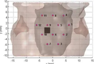
Twelve optodes, arranged in a honeycomb pattern, were located at the top of the head, as shown in Figure 8, resulting in 132 source-detector combinations. The optode configuration is the same as that used in real experiments.

Figure 8 Top view of optode locations. The black object indicates the location of the active area.

An inclusion, embedded in the brain, was specified to model a perturbation. This type of localized change is representative of stimulation experiments involving whisker pad or paw stimulation. Absorption values corresponding to nodes lying inside the object were specified by sampling the quasi-periodic function (12). As before, the measurement strategy consisted of using sequentially one optode for light delivery and the remaining optodes for collection. The full 3D FEM model given by equations (2)-(4) was simulated to generate optode measurements to the dynamic behaviour of the inclusion given by the quasi-periodic signal in equation (12).

4.2 Solution of the Inverse Problem

A separate mesh was constructed for image reconstruction. The MRI scans used to derive the initial mesh used to compute synthetic measurements were subsampled and cropped, then converted into a mesh consisting of 23424

nodes and 117550 tetrahedral elements, as shown in Figure 9. Following the standard FEM-based approach, images are reconstructed using the inverse mesh (Figure 9

c)

through an optimization scheme; however, for the proposed method the reduced model needs to be calculated before the inverse problem is solved. To this end, input and output data used to estimate and validate the reduced order model was generated by simulating the 3D FEM approximation of the forward model (2)-(4) on the inverse mesh.

Since absorption changes due to brain activation cannot occur in skin or bone and since for a particular experiment, it is often possible to define a Region of Interest (ROI) (where changes of optical parameters are expected to occur), a reduced-order ROI-specific model can be derived for a particular study.

In this particular example, the ROI, which comprises 576 nodes, is shown in Figure 10. For each node within the region of interest, 1000 normally distributed values of absorption changes relative to the baseline were generated independently. Predicted optode measurements were computed for each of the 1000 sample distributions of absorption variations in the target area.

4.3 Model Estimation and Validation

The first 500 samples were used as estimation data and the remaining data set was used for validation. For each source-detector pair, a polynomial model was estimated using the OFR algorithm based on a second order polynomial model. The dimension of the parameter space is 576 resulting in a set of 166752 candidate terms. The PDMF function was used to guide the structure detection algorithm. In effect, the original model set of 166752 candidate terms was reduced to a range between ~400 to ~30000, depending of the source-detector separation. The cross–validation technique, described earlier, was used to determine the ERR cut-off points for each source-detector model. The final reduced-order forward model consisted of 132 equations, each equation corresponding to a source-detector combination. The number of terms in each equation ranged between 15 and 100.

(a) (b) (c) Figure 9 Coarse mesh generation. (a) Downsampled and cropped MRI image, (b) 3D model after segmentation and

Figure 10 ROI is defined by the embedded object located at the top of the brain.

4.4 Three-Dimensional Image Reconstruction Using the Reduced Forward Model

Image reconstruction was constrained to the ROI shown in Figure 10, i.e. only absorption changes for nodes lying within the constraint region were estimated. Image reconstruction was performed using the CGD algorithm based on the full FEM model and the reduced order model. For the FEM-based reconstruction algorithm, the reconstruction error given by equation (7) converged after 30 minutes (11 iterations). The image correlation coefficient of the reconstructed image was ICCFEM=0.75.

In contrast, image reconstruction using the reduced model required only 6 iterations and took less than 1 second. However, the quality of the image reconstructed based on the reduced order model is lower compared to the FEM solution ICCROM=0.64. This is clearly due to the

approximation error introduced by the reduced order model. This disadvantage is amply compensated by considerable computational speed-up of more than 900 times (from 30 minutes to less than 2 seconds - assuming 11 iterations for the reduced order algorithm).

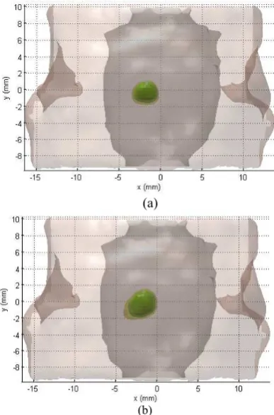
Three dimensional reconstruction of the inclusion using the FEM-based approach is displayed in Figure 11a. The contours correspond to signal amplitude thresholds of 50%, 60% and 70% of the maximum estimated variation. Figure 11b illustrates the reconstruction achieved based on the reduced model

A point at the centre of the inclusion was selected to show the reconstruction of the dynamic changes using both methods. The behaviour of the absorption changes for this point is displayed in Figure 12a along with the original perturbation signal. Figure 12b shows the ICC for the complete signal using both methods.

The means are ICCFEM =0.74for the FEM-based reconstruction and ICCROM=0.64for the reduced model approach. This corresponds to a ~14% reduction of the correlation index for the reduced model approach. However, the index is consistent through the whole experiment.

In practice, the reconstruction error introduced by the reduced model can be made arbitrarily small by employing a higher order polynomial approximation scheme, whilst maintaining the reconstruction speed.

(a)

(b)

Figure 11 Recovered inclusion using (a) the full FEM model and (b) the reduced order model.

0 50 100 150 200

-1 0 1 2

x 10-3

Time point

Δ

μa

Original perturbation FEM-based reconstruction Reduced model reconstruction

(a)

0 50 100 150 200

0.5 0.6 0.7 0.8 0.9

Time point

Im

a

g

e

c

o

rr

e

la

ti

o

n

c

o

e

ff

ic

ie

n

t

FEM-based reconstruction Reduced model reconstruction

(b)

Figure 12 (a) Reconstruction of the complete time series. (b) Image correlation coefficient for each time point.

5. Conclusions

problems. The images reconstructed using the proposed approach, are very similar in quality with those obtained using the standard approach, but obtained at a fraction of the time – a speed up of about 900 was achieved on the 3D reconstruction problem.

The new approach offers the possibility to perform high quality 3D tomographic reconstruction in real time using commercially available CW optical tomography instruments such as NIRx [9].

In this study, tomographic reconstruction was carried out, on purpose, on a rather modest computer to demonstrate the fact that the proposed approach does not require multi-core processing to achieve a reconstruction frame rate of several Hz.

Acknowledgements

The authors gratefully acknowledge the support from the EPSRC and an ERC Advanced Investigation Award. E. E. Vidal-Rosas gratefully acknowledges the support from a grant of the Mexican National Research Council for Science and Technology (CONACYT).

References

[1] S. R. Arridge, "Optical tomography in medical imaging," Inverse Problems, 15(2), 1999, R41-R93.

[2] S. A. Billings, S. Chen & M. J. Korenberg, "Identification of MIMO non-linear systems using a forward-regression orthogonal estimator," International Journal of Control, 49(6), 1989, 2157-2189.

[3] S. A. Billings & W. S. F. Voon, "Structure detection and model validity tests in the identification of nonlinear systems," IEE Proceedings D: Control Theory and Applications, 13(4), 1983, 193-199.

[4] A. Y. Bluestone, M. Stewart, J. Lasker, G. S. Abdoulaev, & A. H. Hielscher, "Three-dimensional optical tomographic brain imaging in small animals, part 1: hypercapnia," Journal of Biomedical Optics, 9(5), 2004, 1046-1062.

[5] M. E. Eames, B. W. Pogue, P. K. Yalavarthy, & H. Dehghani, "An efficient Jacobian reduction method for diffuse optical image reconstruction," Optics Express, 15(24), 2007, 15908-15919.

[6] A. P. Gibson, J. C. Hebden, & S. R. Arridge, "Recent advances in diffuse optical imaging," Physics in Medicine

and Biology, 50(4), 2005, R1-R43.

[7] H. L. Graber, Y. L. Pei, & R. L. Barbour, "Imaging of spatiotemporal coincident states by DC optical tomography," IEEE Transactions on Medical Imaging,

21(8), 2002, 852-866.

[8] M. Guven, B. Yazici, X. Intes, and B. Chance, "Diffuse optical tomography with a priori anatomical information,"

Physics in Medicine and Biology, 50(12), 2005,

2837-2858.

[9] NIRx Technologies, LLC. http://www.nirx.net/ [10] J. Nocedal, S. Wright, Numerical optimization

(New York: Springer, 2006).

[11] K. D. Paulsen & H. B. Jiang, "Spatially Varying Optical Property Reconstruction Using a Finite-Element Diffusion Equation Approximation," Medical Physics,

22(6), 1995, 691-701.