Errors in predicting furrow irrigation performance using single measures of infiltration 1
P.K. Langat, S.R. Raine and R.J. Smith 2
3
Abstract 4
Commercial performance evaluations of surface irrigation are commonly conducted using 5
infiltration functions obtained at a single inflow rate. However, evaluations of alternative 6
irrigation management (e.g. flow rate, cut-off strategy) and design (e.g. field length) options 7
using simulation models often rely on this single measured infiltration function, raising 8
concerns over the accuracy of the predicted performance improvements. Measured field data 9
obtained from 12 combinations of inflow rate and slope over two irrigations were used to 10
investigate the accuracy of simulated surface irrigation performance due to changes in the 11
infiltration. Substantial errors in performance prediction were identified due to (a) infiltration 12
differences at various inflow rates and slopes and (b) the method of specifying the irrigation 13
cut-off. Where the irrigation cut-off at various inflow rates was specified as a fixed time 14
identified from simulations using the infiltration measured at a single inflow rate, then the 15
predicted application efficiency was generally well correlated with the application efficiency 16
measured under field conditions at the various inflow rates. However, the predictions of 17
distribution uniformity were poor. Conversely, specifying the irrigation cut-off as a function 18
of water advance distance resulted in adequate predictions of distribution uniformity but poor 19
predictions of application efficiency. Adjusting the infiltration function for the change in 20
wetted perimeter at different inflow rates improved the accuracy of the performance 21
predictions and substantially reduced the error in performance prediction associated with the 22
Introduction 1
Surface irrigation efficiency is affected by a range of factors including the inflow rate, soil 2
infiltration characteristic, field length, target application volume, period of irrigation, surface 3
roughness and field slope (e.g Walker and Skogerboe, 1987; Pereira and Trout, 1999). 4
Furrow length and field slope are commonly considered design factors that are not easily 5
modified. Similarly, the soil infiltration characteristic and surface roughness are essentially 6
fixed factors over which the irrigator has limited, if any, control. However, inflow rates, 7
target application volume and time to irrigation cut-off are generally considered management 8
factors which can be varied between events by the irrigator and hence, used to improve 9
irrigation performance. 10
11
The soil infiltration characteristic is one of the most important determinants of surface 12
irrigation performance (McClymont and Smith, 1996; Oyonarte et al., 2002). However, 13
infiltration often varies temporally and spatially and thus makes the management of surface 14
irrigation a complex process (Camacho et al., 1997; Raghuvanshi and Wallender, 1997; 15
Rasoulzadeh and Sepaskhah, 2003). The adjustment of furrow inflow rates and cut-off times 16
is commonly used under commercial conditions to optimize irrigation performance in 17
response to changes in soil infiltration and target application volumes (Raghuvanshi and 18
Wallender, 1997; Raine et al., 1997 & 1998; Smith et al., 2005; Zerihun et al., 1996). 19
However, the optimization of surface irrigation performance typically involves the use of 20
field data often obtained from a single irrigation event. 21
22
Measured irrigation advance data is commonly used to calculate the soil infiltration function 23
using an inverse solution of the volume balance equation (e.g. Walker and Skogerboe, 1987; 24
within a simulation model to reproduce the measured irrigation in a calibration-validation 1
process (Pereira and Trout, 1999; Raine et al., 2005). Assuming adequate model calibration, 2
alternative irrigation strategies (e.g. flow rates and time to cut-off) are then evaluated to 3
identify an appropriate “optimal” irrigation recommendation. 4
5
The only commercial surface irrigation evaluation service currently provided in Australia 6
(Raine et al., 2005) uses the surface irrigation model SIRMOD II (Walker, 2001). The 7
service undertakes field evaluations and provides recommendations on improved 8
management and design parameters. While there are a range of options available, the most 9
common service involves measuring a single irrigation (i.e. single flow rate and infiltration 10
condition) and using this data to make recommendations regarding inflow rate and cut-off 11
time to improve performance. SIRMOD II has the capability to modify the infiltration 12
function based on changes in furrow wetted perimeter and inflow discharge. However, this 13
feature is rarely used in practice due to the parameterization requirements. The failure to 14
adjust the infiltration function in response to changes in the simulated inflow has raised 15
concerns over the accuracy of “optimal” recommendations based on different flow rates and 16
cut-off strategies. Due to labour considerations, recommendations for cut-off are sometimes 17
formulated around labour shifts (e.g. “cut-off after 8 or 12 hours”) rather than based on water 18
advance to specified distances along the field (e.g. “cut-off when water reaches the end of 19
furrows”). Hence, the objectives of this study were to investigate the effect of (a) inflow rate 20
and slope on furrow infiltration, (b) infiltration variation on the accuracy of the irrigation 21
performance prediction when the operator has only measured the infiltration function at a 22
single flow rate and slope and (c) time-based and distance-based irrigation cut-off 23
recommendations on the accuracy of irrigation performance predictions at different inflow 24
1
Method and Materials 2
Evaluation data
3
The field data used in this evaluation was obtained from Mwatha and Gichuki (2000) who conducted
4
furrow irrigation trials in the Bura Irrigation Scheme, Kenya. The soils in the Bura area are shallow
5
sandy clay loams and heavy cracking clays overlying saline and alkaline subsoils of low permeability.
6
The irrigation water is pumped from the Tana River and conveyed through canals to smallholder
7
irrigation fields where it is siphoned into 0.9 m spaced furrows. Data from two irrigations (first and
8
fifth) during the 1989 growing season were collected from four irrigated cotton plots (lengths of
275-9
300 m) with average slopes of 0.09, 0.13, 0.25 and 0.31 % (Table 1). All data was collected from
10
plots located on the same soil type (Mwatha and Gichuki, 2000). The first irrigation had a deficit of
11
70 mm and the fifth irrigation had a deficit of 63 mm as measured by the difference in the volumetric
12
soil moisture content taken at 50 m distances along the field before the irrigation and two days after
13
irrigation (Mwatha and Gichuki, 2000). Within each plot there were three inflow rate (1.5, 2.0 and
14
3.0 Ls-1 furrow-1) treatments and data was collected from four furrows in each treatment. Inflow was
15
measured using Parshall flumes and for the purpose of this analysis it was assumed there was no
16
inflow variability.
17
18
{insert Table 1 near here}
19
20
Computation of infiltration parameters
21
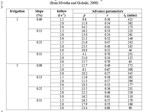
Mwatha and Gichuki (2000) reported the fitted parameters (p and r) for a power function describing
22
the measured water advance (average of four furrows) for each of the irrigation events:
23
x = p(ta)r Equation 1 24
where ta is the time taken for the water to reach advance distance x. These data (Table 1) were used to 25
calculate irrigation advance points and to calculate the fitted parameters (a, k, and fo) for the modified 26
Kostiakov infiltration function using the infiltration model INFILT (McClymont and Smith, 1996):
Z = k(ד)a + ƒo(ד) Equation 2 1
where Z is the cumulative infiltrated volume per unit furrow length (m3 m-1) and ד is the infiltration
2
opportunity time (min). However, large differences in the shape of the infiltration functions were
3
observed possibly due to the short periods of advance data available for some furrows. The a, k and
4
fo parameters are highly inter-related and, particularly where only short periods of advance data are 5
available, there is large uncertainty in these fitted parameters. This may lead to interpretative
6
differences in the shape of the cumulative infiltration function which are related more to the
7
calculation method rather than observed physical differences (Holzapfel et al., 2004). Hence, to
8
ensure that the shape of the infiltration functions were not influenced by the calculation method, the
9
infiltration functions were calculated using a model infiltration function and scaling process (Khatri
10
and Smith, 2006). This approach involved the arbitrary selection of a single measured infiltration
11
function (termed the “model infiltration function”) and the calculation of a scale factor (F) for other
12
events conducted at the same time but on different field slopes and/or with different flow rates.
13
14
The infiltration function calculated for the 2.0 L s-1 and 0.13 % field slope event for each irrigation 15
was selected as the model infiltration function and the modified Kostiakov fitted parameters were
16
calculated using the infiltration model INFILT (McClymont and Smith, 1996). The scaling factor (F)
17
for each of the other treatments was then obtained from the volume balance equation as:
18
r tx f x kt
x A t Q F
o a z
o y o
+ + − =
1 σ
σ
Equation 3
19
where Qo is the inflow rate for the specific furrow (in m3 min-1), σy is a surface shape factor usually 20
taken to be constant at 0.77, a, k, and fo were the modified Kostiakov equation fitted parameters 21
derived for the model infiltration function, r is the exponent from the power curve advance function
22
for the furrow, t is the advance time (in min) for a known advance distance x (in m) in the furrow and
23
σzis the sub-surface shape factor for the model infiltration furrow and calculated as: 24
) 1 )( 1 (
1 ) 1 (
r a
a r a
z + +
+ − + =
σ Equation 4
The cross-sectional area of flow (Ao) was calculated using the furrow geometry measurements 1
provided by Mwatha and Gichuki (2000) and the Manning equation. As all irrigations were
2
conducted on bare furrows the Manning coefficient was assumed to be 0.04 (Walker, 2001). The
3
scale factor was then used to calculate the cumulative infiltration (Z) for the irrigation using:
4
Z = F{k (ד)a + ƒ
o (ד)} Equation 5
5
Both equations 3 and 5 assume that the infiltration variation involves variation of both k and ƒo, an 6
assumption that might not apply to all soils.
7
8
Effect of infiltration function on the accuracy of performance evaluation
9
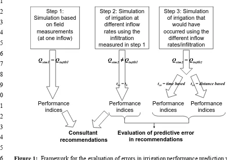
A framework for evaluating the effect on performance of not adjusting the infiltration function in
10
response to changes in inflow is shown in Figure 1. Performance evaluations were conducted using
11
the surface irrigation model SIRMOD II (Walker, 2001) and the performance indices used were the
12
application efficiency (Ea), requirement efficiency (Er) and distribution uniformity (DU) as calculated 13
by SIRMOD II (Walker, 2001). In step 1, the evaluations simulated the measured irrigations by
14
setting the simulation flow rate (Qsim1) equal to the flow rate at which the infiltration function was 15
measured (Qinfilt1). The Manning n value was adjusted from the default value (i.e. n = 0.04) until the 16
simulated advance time at the end of the field was equal to the measured advance time (McClymont et
17
al., 1996). In each case, the adjustments were small (i.e. < 0.02) and within the reasonable values for
18
bare furrows (ASAE, 2003).
19
20
{Insert Figure 1 about here}
21
22
To evaluate the impact of varying Qsim without adjusting the infiltration function (Step 2 of Figure 1), 23
Qsim was then set to either 1.5, 2.0 or 3 L s-1 without changing the infiltration function. It is at this 24
point that commercial consultants commonly make a decision on “optimal” recommendations
25
regarding inflow rates and cut-off times. In this case, the simulation was conducted with the cut-off
26
time (tco) being arbitrarily set equal to the advance time (tL). However, in formulating the cut-off 27
recommendation for the irrigator, the consultant may specify either (a) that the water should be cut-off
after a fixed period of irrigation (i.e. time based), (b) when the water has reached a specified distance
1
along the field (i.e. distance based) or (c) some combination of these methods as when a fixed time is
2
specified after the water has reached the end of the field. Hence, step 3 of this evaluation (Figure 1)
3
involved simulating the irrigation that would have occurred had the grower adopted either a time or
4
distance based recommendation but where the infiltration function used was appropriate to the
5
recommended inflow rate (i.e. Qsim2 = Qinfilt2). The two options for cut-off were simulated: (a) cut-off 6
set equal to the advance time (tL) identified when this flow rate (Qsim2) and the original infiltration 7
function (Qinfilt1) were used in the simulation and (b) cut-off set equal to a specified advance distance 8
(i.e. the end of the field) but when the infiltration function appropriate for this flow rate (i.e. Qinfilt2) 9
was used in the simulation. Evaluations were conducted for each of the 24 combinations of slope and
10
inflow rate for which data was available.
11
12
In this paper, infiltration functions and performance parameters calculated directly from the measured
13
inflow rates and advance data are referred to as the “measured” parameters to distinguish these from
14
the performance parameters obtained from simulations where the simulated inflow rate is different to
15
that at which the infiltration function was calculated. Similarly, the difference in the performance
16
parameters calculated using the measured infiltration functions and where the simulated inflow rate is
17
different to that at which the infiltration function was calculated is referred to as the “error” in
18
performance prediction.
19
20
Effect of adjusting infiltration for wetted perimeter differences
21
The inflow rate applied to furrows influences infiltration by altering both the depth of water in the
22
furrow and the wetted perimeter (Enciso-Medina et al., 1998; Schmitz, 1993). Many workers (e.g.
23
Strelkoff and Souza, 1984; Camacho et al., 1997; Walker, 2001; Mailhol et al., 2005) have suggested
24
that the accuracy of simulated irrigations can be improved by modifying the infiltration function to
25
reflect differences in wetted perimeter at various inflow rates. To evaluate the impact of modifying
26
wetted perimeter on the accuracy of the performance predictions, Step 2 above was repeated but
where the infiltration measured in step 1 was modified according to the approach of Strelkoff and
1
Souza (1984) using:
2
b
sim sim sim
sim
WP WP Z
Z
⎭ ⎬ ⎫ ⎩
⎨ ⎧ =
1 2 1
2 Equation 6
3
where WPsim1 is the wetted perimeter (in m) and Zsim1 is the infiltration at Qsim1, WPsim2 is the wetted 4
perimeter (in m) and Zsim2 is the calculated infiltration adjusted for wetted perimeter at Qsim2 and b is 5
an empirical exponent. In this study, the exponent was assumed to be 0.6 which is consistent with the
6
value proposed by Alvarez (2003) and subsequently used by Mailhol et al. (2005). However,
7
Oyonarte et al. (2002) measured a value of 0.6 for early season events and 0.3 for later season
8
irrigations.
9
10
Results and Discussion 11
Effect of inflow rates and furrow slope on infiltration
12
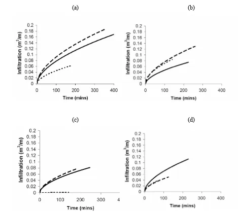
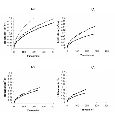
The scaled cumulative infiltration curves (Figure 2 and 3) indicate that infiltration generally 13
increased with increases in inflow rate and decreased with increasing slope. However, the 14
trends were much more consistent for the fifth irrigation (Figure 3) than for the first irrigation 15
(Figure 2). The differences in both the measured advance parameters (Table 1, tL and r)
16
suggest that infiltration variability was larger in the first irrigation and may be masking some 17
of the expected hydraulic effects of changes in flow rate and slope. The larger advance and 18
infiltration variations observed in the first irrigation suggests that the factors (e.g. cultivation, 19
initial soil moisture content) influencing variability were more dominant early in the season. 20
21
The effect of slope and inflow rate on infiltration is broadly consistent with the observations 22
of others (e.g. Holzapfel et al., 2004) and is presumably related to the effect of these factors 23
on flow depth and wetted perimeter. As the slope decreases and the inflow increases the flow 24
for the fifth irrigation events (Figure 3) conducted on higher slopes (>0.13%) there was little 1
difference between the 2.0 and 3.0 L s-1 infiltration functions suggesting that the difference in 2
depth and wetted perimeter for these flow rates was small. However, for the low slope 3
(0.09%), the difference between the infiltration functions at each inflow rate was substantial. 4
5
{Insert Figures 2 and 3 about here} 6
7
Effect of infiltration function on the accuracy of performance evaluation
8
The results of the performance evaluations conducted using the 1.5 L s-1 flow rates on the 9
0.09 and 0.31 % slope plots are shown in Table 2 as an example only. In this example, the 10
performance of the simulations conducted to evaluate the measured irrigation events (i.e. 11
Qsim1 = Qinfilt1) varied substantially with application efficiencies (Ea) ranging from 39 to 99 %,
12
requirement efficiencies (Er) from 80 to 100% and distribution uniformities (DU) from 63 to
13
73%. 14
15
{Insert Table 2 about here} 16
17
Evaluations of performance for different inflow rates using the Qinfilt1 infiltration functions
18
(i.e. Qsim2≠Qinfilt1) generally suggested that substantial improvements in Ea and DU could be
19
obtained by changing inflow rates. However, the actual change in performance that would 20
have been achieved had these inflow rates been applied (i.e. Qsim2 = Qinfilt2) was highly
21
variable and heavily dependent on both the cut-off strategy applied and the difference in the 22
infiltration functions at the two inflow rates. For example, a recommendation to apply 3.0 L 23
s-1 to the 0.09% slope field was predicted to achieve an Ea and DU of 69 and 75 %
24
respectively for the first irrigation, and an Ea and DU of 63 and 75 % respectively for the fifth
irrigation (Table 2). However, for the first irrigation, applying 3.0 L s-1 would have resulted 1
(Qsim2 = Qinfilt2) in an Ea of 65-86 % and a DU of 88-95 % depending on whether the cut-off
2
recommendation was time based or distance based. However, for the fifth irrigation, the 3
same strategies would have produced an Ea of only 27 or 42 % and a DU of 0 or 65 %.
4
Hence, increasing the flow rate in the fifth irrigation event would have reduced the 5
performance rather than increasing it as predicted. Similarly, using a time based cut-off 6
strategy based on the Qinfilt1 simulation would have led the farmer to cut-off the inflow before
7
the water reached the end of the furrow resulting in substantial under-irrigation. 8
9
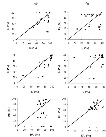
The comparative performance data for all 24 combinations of flow rate and slopes indicate 10
that the error in prediction was generally greater in the first irrigation (Figure 4) than in the 11
fifth irrigation (Figure 5). This is consistent with the larger variability in advance observed 12
(Table 1), and the consequent differences in the infiltration functions calculated for the first 13
irrigation (Figure 2). Hence, variability in infiltration is a significant determinant of 14
performance evaluation accuracy using predictive modelling and suggests that some account 15
of both spatial and temporal variability is required to adequately characterise predictive 16
accuracy at the field scale (Schwankl et al., 2000). 17
18
{Insert Figures 4 and 5 about here} 19
20
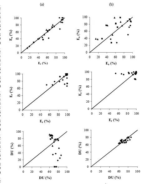
Effect of cut-off recommendation on the accuracy of performance prediction
21
The main effect of the irrigation cut-off strategy recommendation was to trade-off the 22
predictive accuracies of Ea and DU. For the fifth irrigation, approximately 88% of the Ea
23
predictions using the time based recommendation were within 10% of the expected 24
simulations were within ±10% (Figure 5a). Conversely, using the distance based 1
recommendation for cut-off time (Figure 5b) resulted in only 42% of the Ea predictions, but
2
all of the DU predictions, being within ±10% of the values calculated using the infiltration 3
function appropriate to the inflow. 4
5
Time based recommendations for cut-off generally resulted in predictions of Ea which were
6
well correlated with the Ea that would have been obtained using the appropriate infiltration
7
function (Figures 4a and 5a). In this case, volume balance errors associated with the 8
differences in the infiltration function used did not affect the total volume of water applied 9
but did affect the relative proportions of deep drainage and tail water. The main effect of the 10
error in infiltration when using a time based cut-off was the impact on the total distance over 11
which the water advanced. Applying the water for a fixed time on a soil with a larger 12
cumulative infiltration function than used in the prediction resulted in water advances which 13
did not reach the end of the field. In these cases, the lack of water application over 14
substantial areas of the field resulted in widely ranging DU values (0-90%) which were 15
poorly correlated with the predicted DU values (generally 60-90%). 16
17
Distance based recommendations for cut-off generally resulted in predictions of Ea which
18
were poorly correlated with the Ea that would have been obtained using the appropriate
19
infiltration function (Figures 4b and 5b). However, DU was better predicted when the cut-20
off was based on distance rather than time. Using the distance based cut-off recommendation 21
resulted in the whole field being irrigated but reduced the accuracy of prediction for the total 22
water required to be applied. Using a distance based recommendation for cut-off was also 23
found to generally under-predict Er.
24
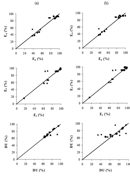
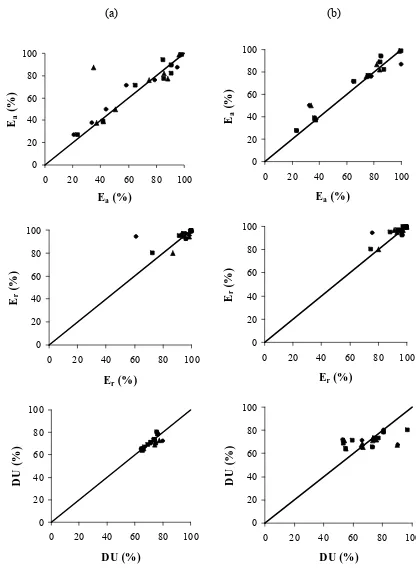
Effect of adjusting infiltration for differences in wetted perimeter
1
Adjusting the infiltration function according to flow rate and wetted perimeter differences 2
was found to substantially improve the accuracy of the performance index prediction (e.g. 3
compare Figures 4 and 5 with Figures 6 and 7). There was also a much reduced effect of the 4
irrigation cut-off strategy (e.g. time based versus distance based) on the accuracy of the 5
performance indices. This suggests that the failure to adjust the infiltration function due to 6
changes in the wetted perimeter was a major determinant of predictive errors in the earlier 7
analyses (e.g. Figures 4 and 5). Residual errors in the performance prediction after 8
adjustment for the wetted perimeter effects could be expected to be due to in-field spatial 9
infiltration variability. The use of the b = 0.6 exponent value in equation 6 would also appear 10
to be appropriate for this soil and contrary to the findings of Oyonarte et al. (2002) there does 11
not appear to be any justification for different exponent values for the early and later 12
irrigations in the season. 13
14
{Insert Figures 6 and 7 about here} 15
16
Conclusions 17
Infiltration functions obtained from 24 combinations of slopes and inflow rates were used to 18
investigate the effect of infiltration differences on the accuracy of simulated surface irrigation 19
performance evaluations. Substantial differences in infiltration were measured between each 20
irrigation event, inflow rate and field slope. The errors in simulated performance were found 21
to be a function of the strategy adopted for irrigation cut-off. Using a time based cut-off 22
strategy generally produced reasonable estimates of Ea but poor estimates of DU.
23
Conversely, distance based cut-off strategies resulted in adequate predictions of DU but poor 24
predictions of Ea. However, where the infiltration was adjusted for changes in the wetted
perimeter at different flow rates, then the accuracy of the performance predictions was 1
substantially improved and the effect of cut-off strategy on the accuracy of the predictions 2
greatly reduced. 3
4
Acknowledgement 5
The data used in this research was collected by Mwatha and Gichuki (2000) and is greatly 6
appreciated. 7
8
References 9
Alvarez RAJ (2003) Estimation of advance and infiltration equations in furrow irrigation for 10
untested discharges. Agricultural Water Management 60: 227-239. 11
ASAE (2003). Evaluation of furrows. ASAE Standard EP419. American Society of 12
Agricultural Engineers, St. Joseph, MI. 13
Camacho E, Perez-Lucena C, Roldan-Canas J, Alcaide M (1997) IPE: Model for 14
management and control of furrow irrigation in real time. Journal of Irrigation and
15
Drainage Engineering123: 264-69.
16
Enciso-Medina J, Martin D, Einsenhaur D (1998) Infiltration model for furrow irrigation. 17
Journal of Irrigation and Drainage Engineering ASCE124(2): 73-80.
18
Gillies MH, Smith RJ (2005). Infiltration parameters from surface irrigation advance and run 19
off data. Irrigation science24:25-35 20
Holzapfel EA, Zuniga C, Jara J, Marino M, Paredes J, Billib M (2004) Infiltration parameters 21
for furrow irrigation. Agricultural Water Management68: 19-32. 22
Khatri KL, Smith RJ (2006) Real-time prediction of soil infiltration characteristics for the 23
management of furrow irrigation. Irrigation Science (in press, DOI 10.1007/s00271-24
Mailhol JC, Ruelle P, Povova Z (2005) Simulation of furrow irrigation practices (SOFIP): a 1
field scale modelling of water management and crop yield for furrow irrigation.
2
Irrigation Science24: 37-48. 3
McClymont DJ, Smith, RJ (1996) Infiltration parameters from the optimisation on furrow 4
irrigation advance data. Irrigation Science17: 15-22. 5
McClymont DJ, Raine SR, Smith RJ (1996) The prediction of furrow irrigation performance 6
using the surface irrigation model SIRMOD. Proc. 13th Conference, Irrigation
7
Association of Australia, 14-16th May, Adelaide. 10 pp. 8
Mwatha S, Gichuki FN (2000) Evaluation of the furrow irrigation system in the Bura 9
Scheme. In Land and Water Management in Kenya: towards sustainable land use, 10
Proc. Fourth National Workshop, Soil and Water Conservation Branch, Ministry of 11
Agriculture and Rural Development & Department of Agricultural Engineering, 12
University of Nairobi. 13
Oyonarte NA, Mateos L, Palomo MJ (2002) Infiltration variability in furrow irrigation. 14
Journal of Irrigation and Drainage Engineering128(1): 26-33. 15
Pereira LS, Trout TJ (1999) Irrigation methods. CIGR Handbook of Agricultural 16
Engineering, Michigan, American Society of Agricultural Engineers. 1: 297 -379. 17
Raghuvanshi NS, Wallender WW (1997). Economic optimization of furrow irrigation. 18
Journal of Irrigation and Drainage Engineering123(5): 377 - 385. 19
Raine SR, McClymont DJ, Smith RJ (1997) The development of guidelines for surface 20
irrigation in areas with variable infiltration. Proceedings of Australian Society of
21
Sugar Technologists19: 293-301. 22
Raine SR, Smith RJ, McClymont DJ (1998) The effect of variable infiltration on design and 23
management guidelines for surface irrigation. Proc. National Soils Conference,
27-24
Raine SR, Purcell J, Schmidt E (2005) Improving whole farm and infield irrigation 1
efficiencies using IrrimateTM tools. In Irrigation 2005: Restoring the Balance. Proc.
2
Nat. Conf. Irrig. Assoc. Aust., 17th -19th May, Townsville. 5pp.
3
Rasoulzadeh A, Sepaskhah AR (2003) Scaled infiltration equations for furrow irrigation. 4
Biosystems Engineering 86(3): 375-383. 5
Schmitz GH (1993) Transient infiltration from cavities. I. Theory. Journal of Irrigation and
6
Drainage Engineering ASCE119(3): 443-457.
7
Schwankl L, Raghuvanshi NS, Wallender WW (2000) Furrow irrigation performance under 8
spatially varying conditions. Journal of Irrigation and Drainage Engineering126(6):
9
355-361. 10
Smith RJ, Raine SR, Minkevich J (2005) Irrigation application efficiency under surface 11
irrigated cotton. Agricultural Water Management71: 117-30. 12
Strelkoff TM, Souza F (1984) Modelling effect of depth on furrow infiltration. Journal of
13
Irrigation and Drainage Engineering 110(4): pp 375- 14
Walker WR (2001) SIRMOD II - Surface irrigation simulation, evaluation and design. User's 15
guide and technical documentation., Utah State University, Logan, UT. 16
Walker WR, Skogerboe GV (1987) Surface irrigation: theory and practice. New Jersey, 17
Prentice-Hall Inc. Englewood Cliffs. 18
Zerihun D, Feyen J, Reddey JM (1996) Sensitivity analysis of furrow irrigation parameters. 19
Journal of Irrigation and Drainage Engineering, ASCE122(1):49-57
1 2 3 4 5 6 7 8 9 10 11 12 13 14 15
Figure 1: Framework for the evaluation of errors in irrigation performance prediction when 16
the infiltration function is not adjusted in response to changes in inflow rate 17
18 19 20 21
Step 1: Simulation based
on field measurements
(at one inflow)
Step 2: Simulation of irrigation at different inflow rates using the
infiltration measured in step 1
Step 3: Simulation of irrigation that
would have occurred using the
different inflow rates/infiltration
Qsim1= Qinfilt1 Qsim2≠Qinfilt1
Performance indices
Performance indices
Performance indices
Consultant recommendations
Qsim2= Qinfilt2
tco= time based tco= distance based
Performance indices
Evaluation of predictive error in recommendations
(a) (b) 1
2 3 4 5 6 7 8 9 10 11 12 13 14 15 16
(c) (d)
[image:17.595.62.531.64.486.2]17 18 19 20 21 22 23 24 25 26 27 28 29 30 31
Figure 2: Scaled cumulative infiltration curves for the first irrigation of the season 32
applied to field slopes of (a) 0.09 % (b) 0.13 % (c) 0.25 % and (d) 0.31 % 33
where the inflow rate was 1.5 (―), 2.0 (– –) or 3.0 l s-1 (▪▪▪)
34
35
36
37
38
39
40
1
2
(a) (b)
3 4 5 6 7 8 9 10 11 12 13 14 15 16 17 18
(c) (d)
[image:18.595.86.521.96.532.2]19 20 21 22 23 24 25 26 27 28 29 30 31 32
Figure 3: Scaled cumulative infiltration curves for the fifth irrigation of the season 33
applied to field slopes of (a) 0.09 % (b) 0.13 % (c) 0.25 % and (d) 0.31 % 34
where the inflow rate was 1.5 (―), 2.0 (– –) or 3.0 l s-1 (▪▪▪)
35
36 37
38
Table 1: Advance parameters for the measured irrigation events 1
(from Mwatha and Gichuki, 2000) 2
3
Advance parameters Irrigation Slope
(%)
Inflow
(l s-1) p r tL (mins)
1.5 9.6 0.56 425 2.0 11.8 0.54 362 0.09
3.0 34.5 0.41 173 1.5 16.2 0.53 223 2.0 13.8 0.54 261 0.13
3.0 21.3 0.52 146 1.5 21.6 0.47 242 2.0 23.3 0.48 185 0.25
3.0 38.8 0.52 46 1.5 4.1 0.78 231 2.0 21.0 0.54 125 1
0.31
3.0 15.7 0.70 63 1.5 12.7 0.49 572 2.0 6.1 0.67 308 0.09
3.0 10.2 0.57 345 1.5 12.6 0.56 262 2.0 11.3 0.57 290 0.13
3.0 18.3 0.53 177 1.5 13.5 0.56 231 2.0 22.2 0.46 256 0.25
3.0 16.2 0.61 110 1.5 16.5 0.55 179 2.0 17.9 0.53 186 5
0.31
3.0 13.4 0.68 90
Table 2: Example of the effect of infiltration function and inflow rate on the accuracy of performance evaluations for the (a) first and (b) fifth
1
irrigation event 2
3
0.09 % slope 0.31 % slope
Performance indices
(%)
Performance indices
(%) Evaluation
framework
component Simulation strategy
Qsim
(L s-1)
Qinfilt
(L s-1)
tco
(min) Ea Er DU
tco
(min) Ea Er DU
(a)
Step 1 Qsim1 = Qinfilt1 where tco= tL 1.5 1.5 526 39 100 63 421 48 99 63 Step 2 Qsim2≠Qinfilt1 where tco= tL 2 1.5 297 51 99 67 237 64 98 67
3 1.5 145 69 99 75 116 85 96 75
Step 3 Qsim2 = Qinfilt2 where tco = tco estimated in step 2 above 2 2 297 45 87 30 237 65 100 83
3 3 145 65 93 95 116 72 82 93
Qsim2 = Qinfilt2 where tco = tL 2 2 410 37 98 64 151 93 91 69
3 3 78 86 66 88 64 90 57 84
(b)
4
Step 1 Qsim1 = Qinfilt1 where tco= tL 1.5 1.5 529 39 100 64 166 99 80 73 Step 2 Qsim2≠Qinfilt1 where tco= tL 2 1.5 314 49 100 68 106 97 67 79
3 1.5 161 63 100 75 62 88 54 86
Step 3 Qsim2 = Qinfilt2 where tco = tco estimated in step 2 above 2 2 314 43 88 35 106 100 70 18
3 3 161 42 66 0 62 100 70 33
Qsim2 = Qinfilt2 where tco = tL 2 2 407 38 100 66 168 87 94 72
1
(a) (b)
[image:21.595.54.489.78.643.2]2 3 4 5 6 7 8 9 10 11 12 13 14 15 16 17 18 19 20 21 22 23 24 25 26 27 28 29 30 31 32 33 34 35 36 37 38 39 40 41 42 43
Figure 4: Effect of the inflow rate (● = 1.5; ■ = 2.0; ▲ = 3 L s-1) at which the infiltration 44
was estimated on accuracy of performance predictions for the first irrigation where 45
recommendations for cut-off were specified by (a) time and (b) distance. The x-axis value 46
was simulated with Qsim2 = Qinfilt1 and the y-axis was simulated with Qsim2 = Qinfilt2
47 48 49 50 0 20 40 60 80 100
0 20 40 60 80 100
Ea (%) Ea (% ) 0 20 40 60 80 100
0 20 40 60 80 100
Ea (%)
Ea (% ) 0 20 40 60 80 100
0 20 40 60 80 100
Er (%) Er (% ) 0 20 40 60 80 100
0 20 40 60 80 100
Er (%) Er (% ) 0 20 40 60 80 100
0 20 40 60 80 100
DU (%) DU ( % ) 0 20 40 60 80 100
0 20 40 60 80 100
DU (%)
DU
(
%
(a) (b) 1 2 3 4 5 6 7 8 9 10 11 12 13 14 15 16 17 18 19 20 21 22 23 24 25 26 27 28 29 30 31 32 33 34 35 36 37 38 39 40 41 42
Figure 5: Effect of the inflow rate (● = 1.5; ■ = 2.0; ▲ = 3 L s-1) at which the infiltration 43
was estimated on accuracy of performance predictions for the fifth irrigation where 44
recommendations for cut-off were specified by (a) time and (b) distance. The x-axis value 45
was simulated with Qsim2 = Qinfilt1 and the y-axis was simulated with Qsim2 = Qinfilt2
46 47 0 20 40 60 80 100
0 20 40 60 80 100
Ea (%) Ea (% ) 0 20 40 60 80 100
0 20 40 60 80 100
Ea (%)
Ea (% ) 0 20 40 60 80 100
0 20 40 60 80 100
Er (%) Er (% ) 0 20 40 60 80 100
0 20 40 60 80 100
Er (%) Er (% ) 0 20 40 60 80 100
0 20 40 60 80 100
DU (%) DU ( % ) 0 20 40 60 80 100
0 20 40 60 80 100
DU (%)
DU
(
%
(a) (b) 1 2 3 4 5 6 7 8 9 10 11 12 13 14 15 16 17 18 19 20 21 22 23 24 25 26 27 28 29 30 31 32 33 34 35 36 37 38 39 40 41 42 43 44 45 46 47 48 49 50 51 52 53 54 55 56
Figure 6: Effect of the inflow rate (● = 1.5; ■ = 2.0; ▲ = 3 L s-1) at which the infiltration 57
was estimated on accuracy of performance predictions for the first irrigation where 58
recommendations for cut-off were specified by (a) time and (b) distance. The x-axis value 59
was simulated with Qsim2 = Qinfilt1 where Qinfilt1 was adjusted for changes in wetted perimeter
60
and the y-axis was simulated with Qsim2 = Qinfilt2
61 0 20 40 60 80 100
0 20 40 60 80 100
Ea (%) Ea (% ) 0 20 40 60 80 100
0 20 40 60 80 100
Ea (%) Ea (% ) 0 20 40 60 80 100
0 20 40 60 80 100
Er (%) Er (% ) 0 20 40 60 80 100
0 20 40 60 80 100
Er (%) Er (% ) 0 20 40 60 80 100
0 20 40 60 80 100
DU (%) D U (% ) 0 20 40 60 80 100
0 20 40 60 80 100
DU (%)
DU (
%
(a) (b) 1 2 3 4 5 6 7 8 9 10 11 12 13 14 15 16 17 18 19 20 21 22 23 24 25 26 27 28 29 30 31 32 33 34 35 36 37 38 39 40 41 42 43 44 45 46 47 48 49 50 51 52 53 54 55 56
Figure 7: Effect of the inflow rate (● = 1.5; ■ = 2.0; ▲ = 3 L s-1) at which the infiltration 57
was estimated on accuracy of performance predictions for the fifth irrigation where 58
recommendations for cut-off were specified by (a) time and (b) distance. The x-axis value 59
was simulated with Qsim2 = Qinfilt1 where Qinfilt1 was adjusted for changes in wetted perimeter
60
and the y-axis was simulated with Qsim2 = Qinfilt2
61 62 63 0 20 40 60 80 100
0 20 40 60 80 100
Ea (%) Ea (% ) 0 20 40 60 80 100
0 20 40 60 80 100
Ea (%) Ea (% ) 0 20 40 60 80 100
0 20 40 60 80 100
Er (%) Er (% ) 0 20 40 60 80 100
0 20 40 60 80 100
Er (%) Er (% ) 0 20 40 60 80 100
0 20 40 60 80 100
DU (%) DU ( % ) 0 20 40 60 80 100
0 20 40 60 80 100
DU (%)
DU (
%