A parallel updating scheme for approximating and optimizing high fidelity computer simulations

A parallel updating scheme for approximating and optimizing

high fidelity computer simulations

A. S´obester, S.J. Leary and A.J. Keane

Abstract Approximation methods are often used to construct surrogate models, which can replace expensive computer simulations for the purposes of optimization. One of the most important aspects of such optimization techniques is the choice of model updating strategy. In this paper we employ parallel updates by searching an expected improvement surface generated from a radial basis function model. We look at optimization based on standard and gradient-enhanced models. GivenNp

pro-cessors, the best Np local maxima of the expected

im-provement surface are highlighted and further runs are performed on these designs. To test these ideas, simple analytic functions and a finite element model of a simple structure are analysed and various approaches compared. Key words gradient-enhanced approximations, parallel optimization, radial basis functions

1

Introduction

The problem of optimization using high fidelity computer simulations is common to many engineering design prob-lems. These simulations are based on mathematical mo-dels of some system of interest. Examples include finite e-lement (FE) analysis for structural engineering problems or Navier-Stokes models in computational fluid dynamics (CFD). Optimization is a highly repetitive process requir-ing many analyses of the model under consideration. If Received: 13 November 2002

Revised manuscript received: 14 October 2003 Published online: 29 June 2004

Springer-Verlag 2004

A. S´obesteru, S.J. Leary and A.J. Keane

C.E.D.G., School of Engineering Sciences, University of South-ampton, SouthSouth-ampton, SO17 1BJ, U.K.

e-mail:[email protected]

Revised version of the paper presented at the Third ISSMO/AIAA Internet Conference on Approximations in Op-timization October 14–25, 2002

this model itself is computationally expensive, direct op-timization algorithms can rarely be employed, as a highly repetitive analysis of a high fidelity model becomes too time consuming to be practical.

To overcome this problem cheap approximating mo-dels (often termed “surrogate momo-dels”) are sought. These are based on a limited number of calls to the high fi-delity model. Once constructed, the surrogate model can replace the original high fidelity model for the purposes of optimization.

The first strategic decision that needs to be made relates to the design of experiments (DoE) to be used to provide training data for the approximation method. There are many such methods available to the designer – we will briefly review some of them in the next section. Their common feature is that they try to fill the design space in some sense, as it is commonly recognized that in the absence of any a priori knowledge on the prob-lem under consideration, uniformity of the design points throughout the region of interest is favourable.

Regarding the approximation methods, these can be applied locally or globally. Local approximations, such as polynomial response surfaces (see, e.g. Myers and Mont-gomery 1995), are defined over a specific region of inter-est, namely about the current best design. Optimization proceeds using a move limit or trust region strategy: we optimize only over the region where the model is valid. Successive local approximations are used to guide the search to a stationary point. Convergence is guaranteed, although only to a local optimum.

Global approximations on the other hand try to cap-ture the behaviour of the overall design space. It may be possible to use polynomial response surfaces, but only if the underlying global response is of low modality. Typic-ally, more global approximators are required. Examples include artificial neural networks (Whiteet al.1992), ra-dial basis functions (Powell 1987) and kriging (Sackset al.

1989). In this paper we are particularly concerned with global approximations.

cost. For example, a perturbation analysis of a finite element model may yield these derivatives at very lit-tle cost; in an adjoint CFD model, all the components of the objective function gradient are usually available at a cost of around one function evaluation. This infor-mation can be included in many approxiinfor-mation models. For example Chung and Alonso (2001) and van Keulen and Vervenne (2002) have considered gradient-enhanced polynomial response surfaces and Morris et al. (1993), Chung and Alonso (2002) and Learyet al.(to appear) use gradient-enhanced kriging models. In this paper we con-centrate on the radial basis function approach.

Once a particular approximation has been built, some updating strategy needs to be defined. The simplest is to optimize the approximation, re-evaluate the high fidelity model at the predicted optimum and repeat. This pro-cedure may stall early due to, for instance, the presence of local minima in the underlying function, depending on the global accuracy of the initial surrogate model. If the goal is to improve the quality of the prediction, then a search over prediction error (if available) may be consid-ered. Such an approach can be found in Martin and Simp-son (2002). Given both a prediction and some estimate of the error in the prediction, elegant global optimization strategies can be devised. An example of this is the notion of global search based on expected improvement (see, e.g. Jones et al.1998), which balances the need for a surro-gate objective value together with the uncertainty of the model. This idea can be amended to search more glob-ally, as in Sasenaet al. (2002). Another method would be to weight the objective and uncertainty components of the expected improvement function in order to drive the search more towards optimization or approximation, depending upon the designer’s goals. An expected im-provement function for gradient-enhanced kriging models is presented by Learyet al.(to appear).

Considering that in today’s industrial setting it is commonplace for parallel computing architectures to be available to the design engineer, we advocate the use of parallel computing throughout the design process based on the methods described above. We will assumeNp pro-cessors are available; first these will be used to run our design of experiments in parallel. This information will then be used to construct a surrogate model. Both tradi-tional and gradient-enhanced models will be considered. We will compare the approaches assuming gradients are free and alternatively that they are available at the cost of one function evaluation (which we sometimes term the “adjoint cost”) as both these situations can arise in prac-tice. We note that the use of gradient-enhanced models typically depends on the cost of the gradient: it does not make sense to use gradient enhanced models if the gradi-ents are evaluated using finite differencing.

The updates to the model are also performed in paral-lel: we can either search values of the surrogate objective in order to attempt to quickly optimize the model, search areas of high error in order to globally reduce the model’s error, or search some expected improvement or weighted

expected improvement model. In all these cases either a local optimizer with multiple restarts or a genetic al-gorithm with clustering and sharing could be considered. The idea is either to locate theNpbest optima of the re-sponse surface, theNpdesigns with the highest prediction errors or the Np designs with the highest expected im-provements.

The latter two goals tend to be extremely multimodal. However, ifNpunique minima are not available, we could add some extra points using either of the other two crite-ria. In this paper we consider an expected improvement approach alone as in all the examples tested we always found more local maxima of the expected improvement surface than available processors. We mention the others for completeness.

The rest of this paper is set out as follows. Section 2 considers design of experiments and approximation me-thods; in particular radial basis function approximation methods will be described. Section 3 introduces our paral-lel updating scheme for surrogate optimization. In Sect. 4 we show some results from our approach and in the fi-nal section conclusions are drawn and areas of further research highlighted.

2

DoE and global model building

Before we build an approximation we require a system-atic means of selecting the set of inputs (called a design of experiments, or DoE) at which to perform a computa-tional analysis. Inkdimensions the 2k_{vertices formed by} the upper and lower bounds of the design space usually provide the bounding box within which the experimen-tal design is created. The idea with DoE is to, in some sense, evenly fill this design space with a limited number of points. As a result many of the algorithms employed are referred to as “space filling” designs.1

Simple experimental designs include 2k full factorial designs which are created by specifying each design vari-able at two levels, the upper and lower bounds on each variable (this design considers every vertex of the de-sign bounding box). 3k_{full factorial designs additionally} include the midpoint of each input. These experimen-tal designs prove expensive for largek so they are often replaced with fractional factorial designs. Several other types of designs can be encountered in the polynomial re-sponse surface literature – the interested reader may wish to consult, e.g. Myers and Montgomery (1995) for further details.

A popular choice for generating an experimental de-sign for deterministic computer experiments is theLatin

1

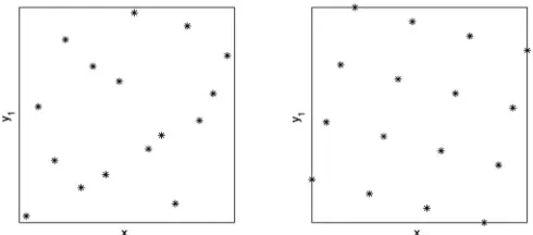
hypercube (Mackay et al.1979). This has the advantage that each of the variables has all portions of its range represented equally. The downside of Latin hypercube designs is that they are not guaranteed to have good space-filling properties. A possible solution is to use op-timal Latin hypercube designs. These are Latin hyper-cubes that achieve optimality in some space filling sense – for example, a maximin distance criterion (Morris and Mitchell 1995). In this paper our experimental designs are formed from optimal Latin hypercube designs using this criterion. An algorithm for generating such designs can be found in Morris and Mitchell (1995). Examples of a standard and a Morris-optimal Latin hypercube using 16 points with two independent variables are shown in Fig. 1. The optimal Latin hypercube DoE is used here to construct training data, upon which the surrogate models are built.

In this work, as we are dealing with relatively simple problems only, we can afford to create a set of testing data, which is used to assess the accuracy of our approx-imation methods – the results are presented in Tables 1 and 2, Sect. 4.2 (of course, in general, this would not be practical for expensive computer simulations). The test-ing data is created ustest-ing LPτ sequences (Sobol 1979), another space-filling DoE formulation.

Once we have chosen a suitable DoE and evaluated the high fidelity model at this set of inputs, we can con-struct an approximation. In a typical approximation mo-del the relationship between observations (responses) and independent variables on ak-dimensional domainDis ex-pressed as

y=f(x) (1)

wherey is the observed response,xis a vector ofk inde-pendent variables

x= (x1, x2, . . . , xk) (2)

andf(x) is some unknown function. An approximation to this response

ˆ

y= ˆf(x) (3)

is sought. As it will become apparent in the next section, it is also important from the optimization point of view to be able to obtain an error estimate for this approxi-mation. To this end, here we employ a stochastic process-based modelling framework. This may seem counterintu-itive, as physics-based numerical computer experiments, the pillars of the majority of computer-aided design op-timization procedures, are usually deterministic. That is, unlike physical experiments, repeated runs of such simu-lations on the same design return the same figure of merit (objective value) each time. Nevertheless, it can be ar-gued that stochastic process approximation techniques can be employed to model this type of output. The ratio-nale is that, although the physics-based simulation

pro-Fig. 1 A Latin hypercube and an optimal Latin hypercube design

cess itself is deterministic, its output can be viewed as a realization of a stochastic process2.

There are several approaches for building such models – here we choose to work with radial basis functions (RBF) on the grounds that their training is inexpen-sive, yet, as we will see, they are sufficiently accurate for optimization purposes. RBF models attempt to express a complicated landscape as the weighted sum of several simple functions – in the following we describe the model building procedure in more detail.

Assuming that we can afford to run the analysis code N times, we sample the objective for N designs (de-noted by [x(1)_,x(2)_{, . . . ,x}(N)_{]), at which we obtain the}

responsesy= [y(1)_{, y}(2)_{, . . . , y}(N)_{]. Radial basis functions}

can be used to make a prediction ˆy= ˆf(x) at any pointx in the design space and the first step towards this is to choose the basis function centers. To obtain an interpolat-ing model we need at leastN bases. The common choice here is the set of N points where we know the objec-tive function values (i.e. [x(1),x(2), . . . ,x(N)]). The basis functions take the formφ(x−x(i)_{), whereφ(·) is some}

(usually) nonlinear function, the ith _{such function} de-pending on the Euclidean distance betweenxandx(i)_{. As}

we mentioned earlier, the predictor is a linear combina-tion of these basis funccombina-tions, that is,

ˆ

y= ˆf(x) = N

i=1

wiφx−x(i)

. (4)

The coefficientswihave to be found such that the predic-tor interpolates the data. To do this, we are required to satisfy forj= 1, . . . , N:

ˆ

fx(j)= N

i=1

wiφx(j)−x(i)

=y(j). (5)

2

Defining the coefficient vectorw= [w1, w2, . . . , wN]T and the matrixΦi,j=φ(x(i)−x(j)), wherei= 1, . . . , N andj= 1, . . . , N, this can be written asΦw=yT_{. Then,} provided the inverse ofΦexists, the coefficients can be determined by computingw=Φ−1_yT _{and a prediction ˆy} can be made in any pointx(N+1)_{∈Dby computing:}

ˆ

y(N+1)=φw=φΦ−1yT (6)

where

φ=

φx(N+1)−x(1)

, φx(N+1)−x(2)

, . . .

. . . , φx(N+1)−x(N). (7)

Many different basis functions φ(·) could be consid-ered. Throughout this work we have used exponentially decaying Gaussian basis functions

φ(r) = exp−r2/2σ2 (8)

as these are twice differentiable and facilitate the deriva-tion of an expected improvement measure (we will return later to the reasons why these two features are import-ant). The choice of the hyperparameterσ, which governs the regions of influence of each kernel, is important and can affect prediction accuracy. In the work presented in this paper we use aleave-one-out cross validation pro-cedure, searching for the optimum σ over the domain [10−2_,101_{]. This means that for each value ofσwe build}

N RBF models leaving out one of the training points in each case (as though we only hadN−1 points), we com-pute the difference between the true objective value of the currently left out point and the objective predicted by the partial model (which uses the remainingN−1 points) in the same point. The final model is constructed using the σthat minimizes the sum of the squares of these residu-als. Of course, the larger the number of training points, the more reliable the training will be (i.e. it is more dif-ficult to find the bestσ for, say,N= 5 by building the five four-point models, than for N= 50, when the pre-dictions can be based on 49-point leave-one-out models). We consider 15 values ofσlogarithmically spread over the range indicated above. More thorough searches (i.e. a full optimization of the hyperparameterσ) could be consid-ered, but this would increase the computational cost of the training and in the authors’ experience the gain in model accuracy thus achieved is not significant. We also note here that the optimumσis related to the distances between the kernels – the range [10−2,101] is suitable for the case when the problem domain is normalized to D= [0,1]k_{(as in the experiments described here).}

Clearly, more accurate models could be considered; for example, we could allow the selection of a differentσ for each independent variable (as is often done, for ex-ample, in kriging). However, the computational cost of model training then becomes an issue (particularly when we move to gradient-enhanced predictions where consid-erably larger matrices need to be inverted).

Supposing that the sensitivities of the objective func-tionf with respect to the design variablesxiare cheaply available, this information can be used to enhance the radial basis function model. In this case we are seeking an osculating interpolant of the set of known objective value points, i.e. a model determined not only by a set of nodal points (the objective function values), but also by the required slopes in those points (the objective function gradients). Assuming we now define anN(k+ 1) vector of responses as

y=

y(1),∇y(1), y(2),∇y(2), . . . , y(N),∇y(N) T

, (9)

where

∇y(i)= ∂f ∂x1

(xi), ∂f ∂x2

(xi), . . . , ∂f ∂xk

(xi)

, (10)

then we can extend our matrixΦto include the first and second derivatives ofφin much the same way as is done in kriging (see, e.g. Morriset al.1993). This assumes our ba-sis function is at least twice differentiable, another reason for using Gaussian basis functions. A gradient-enhanced radial basis function (GERBF) approximation can then be constructed.

3

Optimization

As we have already mentioned, a common approach to reducing the cost of a global optimization procedure is to make use of cheaper surrogate models, such as the stochastic process model-based global RBF approxima-tion described in the previous secapproxima-tion.

The cornerstone of any optimization strategy based on such low-cost surrogates is the choice of the updating method, i.e. given an initial global model how do we select the next site(s) where the expensive objective will be sam-pled? Perhaps the most obvious strategy is to re-sample in areas that appear promising in terms of the objective function value ˆy predicted by the surrogate model. The success of this approach depends on the quality of the initial approximation. If the initial approximation is accu-rate, it is likely to lead the designer quickly to the global minimum or at least to a very good solution.

A second approach may be to search areas of high es-timated approximation error, i.e. in our case, to choose the design that maximizes the estimated error of the RBF predictor. In order to calculate this, we make use of the fiction discussed earlier, namely that each deterministic responsey(x) is in fact the realization of some stochas-tic process Y(x) (taken here to be a Gaussian random variable). Using the (Gaussian) distributions of theN re-sponses y= [y(1)_{, y}(2)_{, . . . , y}(N)_{] collected so far, it can}

be shown that the mean and the variance of the assumed stochastic process atx(N+1)_are:

ˆ

σ_y2_ˆ(N+1) = 1−φΦ− 1

φT (12)

respectively (for a detailed demonstration see, e.g. Gibbs 1997). As expected, the mean of the assumed Gaussian distribution that we drew ˆy(N+1)from (11) is, in fact, the RBF predictor obtained earlier (6). We will use the vari-ance of this Gaussian distribution (12) as a measure of the likely prediction error at untested sites.

Placing the new design to be evaluated at the global maximum of (12) may not make much sense if the goal is to locate a good design quickly, but it does allow global improvement of the approximating model. One might even consider a hybrid method, where in the early stages we search the errors in order to enhance the ac-curacy during the global exploration phase and then refine locally. Nevertheless, it is by no means obvious whether this approach would be better than simply start-ing with a larger design of experiments and then updat-ing the model locally. Ultimately, this would be problem dependent.

From a global optimization perspective, the tech-nique outlined above amounts toexplorationof the search space, whereas searching the predictor itself (as men-tioned earlier in this section) is equivalent to exploiting currently known promising basins of attraction. Clearly, we need a point selection criterion that balances these two approaches.

As we mentioned earlier, the stochastic processY(x) models our uncertainty about the responsey(x) in the pointx. Denoting the best objective value from the sam-ple evaluated so far byymin= min

y(1)_{, y}(2)_{, . . . , y}(N)_,

a further quantity can be defined: theimprovement

I(x) = max [ymin−Y(x),0] (13)

(Joneset al.1998). This is, of course, also a random vari-able – it models our uncertainty about the amount by whichy(x), the objective function value in the next eval-uated sample point, will improve on the current best objective.

Given a prediction ˆyand an error estimates=σ_yˆ(N+1)

(in a pointx, as per equations (11) and (12)), using Gaus-sian kernels, the expectation of the improvement (or, as it is often termed in the literature, theexpected improve-ment) can be calculated (see, e.g. Schonlau 1997) as:

E(I) = EIF(x) = 

   

(ymin−ˆy)Ψ

ymin−yˆ

s

+sψ ymin−ˆy s

ifs >0

0 ifs= 0 (14)

whereΨ(·) is the standard normal distribution function andψ(·) is the standard normal density function.

The first term of (14) is the predicted difference be-tween the current minimum and the prediction ˆy in x, penalized by the probability of improvement. Hence it is large where ˆy is small (or it is likely to be smaller then

ymin). The second term is large when the errorsis large,

i.e. when there is much uncertainty about whethery will be better thanymin. Thus, as Schonlau (1997) points out,

the expected improvement will tend to be large at a point with predicted value smaller than ymin and/or there is

much uncertainty associated with the prediction. There-fore, expected improvement can be considered as a bal-ance between seeking promising areas of the design space (according to our approximation) and the uncertainty in the model. The global search strategy based on it (i.e. evaluation of initial DoE set, followed by updates in the maxima of the expected improvement surface) has the ad-vantage that it is much less likely to stall than a search over the approximation only (although there are certain pathological cases when it does, see, e.g. Jones 2001). The disadvantage is that it usually takes longer to converge, which could be a drawback if the initial model did turn out to be an accurate one.

When we consider constrained optimization, whether the constraints are approximated or evaluated exactly, the expected improvement function needs to be modified as follows: EIF(x) =                         

(ymin−yˆ)Ψ

ymin−yˆ

s

+sψ ymin−yˆ s

ifs >0 and the (approx. or exact) constraints are satisfied

0

ifs= 0 or if the (approx. or exact) constraints are

violated (15)

Furthermore, in this caseyminshould be taken as the

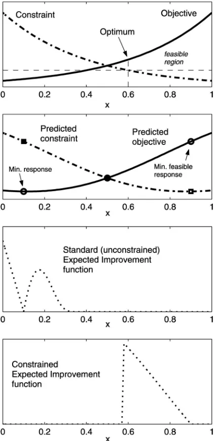
minimumfeasible response. To understand this, consider the simple one-variable demonstrative example shown at the top of Fig. 2.

Assuming without loss of generality that both our ob-jective and constraint are expensive (if our constraint was cheap we would just evaluate it directly), the approxi-mation to these responses based on three sampled values (at x= 0.1,x= 0.5 andx= 0.9) is shown in the second subplot of Fig. 2. Supposing that we are required to min-imize this objective subject to the constraint remaining below the horizontal dashed line (shown on the top sub-plot), the minimum will occur atx= 0.6. If we takeymin

of the figure. In this case our first update is close to the true solution – once this is added to the database of runs and a new approximation is constructed, we quickly home in on this solution.

The optimization strategies outlined above involve re-constructing the surrogate model after each new expen-sive evaluation – therefore the procedures, in their basic form, are sequential. Nevertheless, any of the three strate-gies can also be implemented in parallel – here we choose to work with expected improvement.

Given Np processors, the idea is to locate the Np best local maxima of the expected improvement surface (which is usually extremely multimodal) using, for in-stance, either a gradient-based optimizer with multiple restarts or a genetic algorithm (GA) with clustering and sharing. Once theseNplocal maxima are identified, those

Fig. 2 One-variable demonstrative example of constructing the expected improvement surface in the case of a constrained problem

locations are evaluated in parallel using the high fidelity model and the process is repeated until we converge or run out of time. A flowchart of the approach is shown in Fig. 3.

We could always consider a parallel version of the other model update criteria as well by replacing the ex-pected improvement step in the flowchart with either op-timizing the approximation or its error. As we have men-tioned earlier, if there are not as many optima as there are processors (which is more likely to happen when optimiz-ing the approximation) we could add some points usoptimiz-ing either of the other two approaches.

Furthermore, we could weight the two terms in the ex-pression of the expected improvement (14). As discussed earlier, the first term relates to the approximation and the second to the error. A suitable weighting could be used to bias the search towards one of these, depending on the de-signer’s goals. Once more, this can be done in parallel and the weighting could vary as the search progressed, biasing it towards error reduction to begin with and then moving towards finding an optimal design at the end.

4 Results

4.1

Demonstrative example

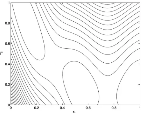
In this section we compare results for the various ap-proaches. To start with we demonstrate our parallel up-dating scheme on the two-variable Branin function. This function is described in the Appendix. It is defined on the domain [−5,10]×[0,15], however we scale these inputs to [0,1]2_{, as highlighted earlier. A contour plot of the Branin}

function is shown in Fig. 4.

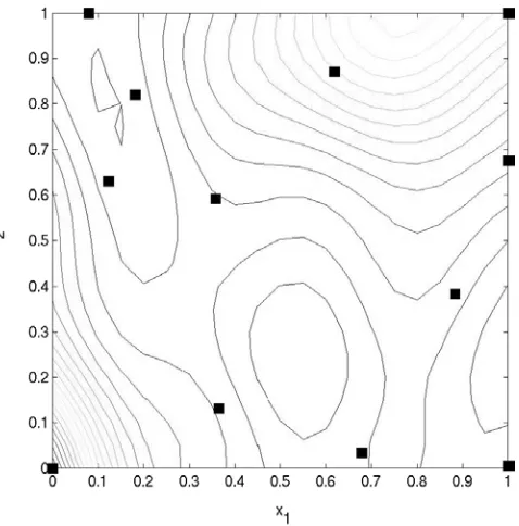
First, using our radial basis function approximation without gradients, assuming four parallel processors, we start with a DoE consisting of eight computer experi-ments (two parallel runs). This is shown in Fig. 5 (top). We then locate the four best maxima of the expected improvement surface, as shown in Fig. 5 (bottom), and re-evaluate the model at these points. We continue until we have 24 points (six parallel runs) – see Fig. 6. The best minimum at this stage is 0.774.

We now consider a gradient-enhanced approxima-tion, assuming that the derivatives are available for free. Again, we assume an initial DoE consisting of eight points (two parallel runs) and perform parallel updates using EIF maximization to locate the next design points. After 24 evaluations (six parallel runs) the approximation is as shown in Fig. 7 and the best minimum is 0.518.

Finally, we assume gradients are available at the cost of one function evaluation. Therefore, our initial DoE here consists of four points. These four function and gra-dient evaluations require two parallel runs. Four new points are found by maximizing the expected improve-ment. The objective function values and the gradients in these points are again evaluated (two parallel runs) and the optimization process is repeated once. The total com-putational cost is equivalent to those above and the best

Fig. 4 Contour plot of the Branin function

Fig. 5 Initial approximation (top) and first EIF maximiza-tion (bottom)

minimum here is 3.589 (Fig. 8). Whilst this is larger than before, it is still a very good objective value considering the range of values the Branin function takes over the domain.

4.2

Results on two five-dimensional test functions

Fig. 6 Approximation to the Branin function after six paral-lel runs

Fig. 7 Approximation to the Branin function assuming free gradients after six parallel runs

defined on the domain [−1,1]5_{and the second, the Ackley}

function, on [−2.048,2.048]5_{. As before, both functions}

are scaled to [0,1]5_.

First we compare the accuracy of the approximating models on one of the test cases. We arbitrarily choose to work with the modified Rosenbrock function. Table 1 shows the accuracy of our radial basis function approx-imation model without gradient information included. The first two columns of the table show the average error and the correlation coefficient (“r2_{-value”) between the}

Fig. 8 Approximation to the Branin function assuming “ad-joint” gradients after six parallel runs

model and the true Rosenbrock function, evaluated at a set of 500 points arranged in an LPτ design. The table also includesσ, the optimum kernel width hyperparame-ter found for each case (see (8)). This data is shown for op-timal Latin hypercube designs of several different sizesN. Table 2 contains the same information using the gradient-enhanced radial basis function (GERBF) approximation. From Tables 1 and 2 it can be seen that as N in-creases our model generally becomes more accurate (the error reduces and the correlation increases), as expected. What is really interesting is to compare the accuracy of the GERBF model with that of the standard RBF model.

Table 1 Accuracy of the approximation without using gradi-ents

N Average error Correlation σ

16 0.7184 0.1412 0.32

32 0.6844 0.2594 0.19

48 0.5925 0.4870 0.19

64 0.5057 0.5540 0.32

80 0.4653 0.6173 0.32

Table 2 Accuracy of the approximation using gradients

N Average error Correlation σ

8 0.6514 0.3625 0.32

16 0.6010 0.4781 0.19

32 0.5536 0.5708 0.19

48 0.3797 0.7355 0.32

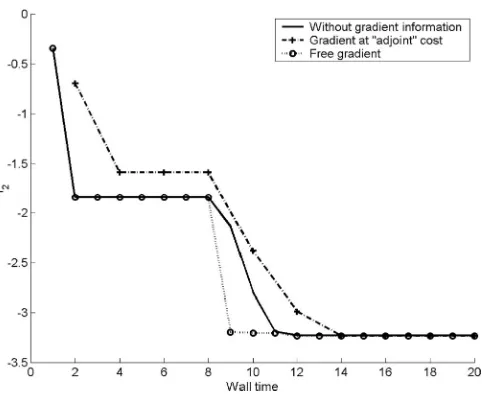
64 0.3336 0.7825 0.32

Fig. 9 Comparison of optimization strategies based on RBF and GERBF models for the modified Rosenbrock function, using one processor

We note that when all the gradients are available at a cost of one function evaluation, utilizing gradient information increases the global accuracy of the model (c.f. Table 1 withN= 16,32 and Table 2 usingN = 8,16). We have observed this to be true for other choices of N, k and other objective functions. When gradients are available virtually for free, the GERBF is far superior.

We now consider how the various approaches perform in terms of optimization. First, we compare the RBF, to-gether with the GERBF, usingNp= 1, 4 and 8 processors on both five design variable objective functions. We look at the performance of the optimization strategy based on these models, assuming gradients are both free and avail-able at a cost of one function evaluation. We choose the size of the DoE so that its computational cost will be the

Fig. 10 Comparison of optimization strategies based on RBF and GERBF models for the modified Rosenbrock func-tion, using four processors

Fig. 11 Comparison of optimization strategies based on RBF and GERBF models for the modified Rosenbrock func-tion, using eight processors

same in each case. We start from a 32-point Latin hyper-cube design in the case of the standard RBF model and the GERBF model when we assume free gradients and a 16-point Latin hypercube design when the gradients are assumed to have “adjoint” cost. Figures 9, 10 and 11 show the results of optimizing the modified Rosenbrock func-tion, usingN p= 1, 4 and 8 processors respectively. Fig-ures. 12, 13 and 14 show the same information when using the Ackley function.

We observe that when we assume gradients are avail-able at adjoint cost, the advantage of using the GERBF for optimization is less obvious than from the approxima-tion point of view (as demonstrated earlier in Tables 1 and 2). If gradients are available for free then their use in optimization unquestionably makes sense.

Fig. 13 Comparison of optimization strategies based on RBF and GERBF models for the Ackley function, using four processors

Fig. 14 Comparison of optimization strategies based on RBF and GERBF models for the Ackley function, using eight processors

One of the most important aspects of such optimiza-tion schemes is the efficiency of the parallelizaoptimiza-tion. As shown in Tables 3 and 4, this varies from case to case. For example, when optimizing the Rosenbrock function using the free gradient-enhanced model, the speedup is nearly linear, whereas in the “adjoint gradient” model-based optimization of the Ackley function, the results on eight processors indicate a sharp drop in efficiency.

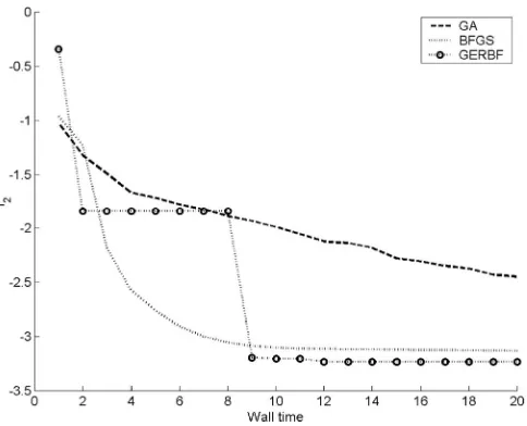
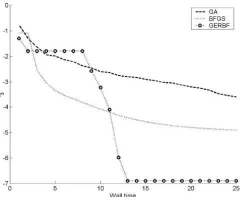
Finally, we consider how these surrogate-based opti-mization strategies perform against some frequently used optimization procedures. Here we assume the gradients are free and consider a GA, a gradient-based method (BFGS) and our optimization scheme utilizing GERBF predictions. Results for both the modified Rosenbrock and Ackley functions are shown in Figs. 15 and 16 respec-tively. Here we arbitrarily useNp= 4.

Table 3 Comparison of number of evaluations (i.e. wall time×Np) needed to reach convergence for the modified Rosenbrock function

Np Without grad. “Adjoint” grad. Free grad.

1 47 40 39

4 48 56 48

8 64 80 40

Table 4 Comparison of number of evaluations (i.e. wall time×Np) needed to reach convergence for the Ackley func-tion

Np Without grad. “Adjoint” grad. Free grad.

1 66 60 39

4 64 64 52

8 80 112 48

The GA and BFGS convergence histories are averaged over 50 optimization runs. When we consider the GA, new members of the population are spread over the Np processors to make use of the parallel computing architec-ture. When considering BFGS we perform one optimiza-tion run on each processor, therefore we are using four random restarts. Multiple restarts are generally required when using gradient-based optimizers, as they become trapped in local minima. The convergence histories show the best objective function value found so far after each parallel run. Finally, we compare these approaches to the GERBF-based optimization approach (again, using four processors).

The results can be summarized as follows. In these cases the GA optimization performs relatively poorly; it is at an obvious disadvantage, as it makes no use of the free gradient information. The BFGS method performs much better: it is almost competitive with our GERBF

Fig. 16 Comparison of optimization techniques on the Ack-ley function with free gradients

based optimization approach on the modified Rosenbrock function, however it does often become trapped in one of the local minima, hence it usually converges to a higher value. On the more strongly multimodal Ackley func-tion the BFGS method performs much worse, often be-coming trapped in local minima and also converging to these minima at a slower rate. Our expected improvement approach using GERBF-based optimization consistently finds the global minimum very quickly. Our conclusions were similar when we considered gradients at “adjoint” cost.

4.3

Structural optimization example

With many finite element models the derivatives with respect to the design parameters can be available very cheaply. For example Haftka (1993) presents a semi-a-nalytic method, whereby sensitivities can be obtained at a fraction of the cost of the analysis itself.

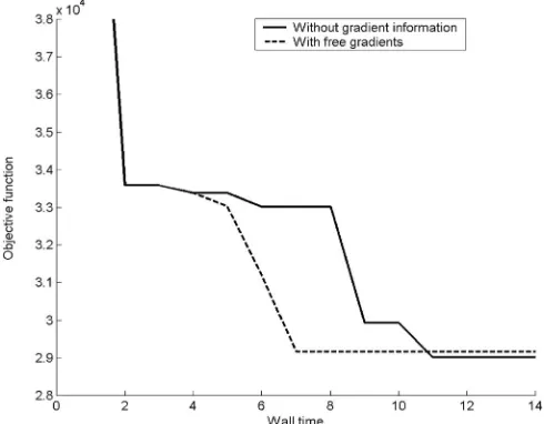
In this final example we consider optimization of the spoked structure shown in Fig. 17 (left). This model is made up entirely of beam elements the thickness of which can be altered in a variety of ways. The part of the struc-ture being optimized is shown on the right of the figure. Six design parameters define the geometry, five of which describe the ring cross section whilst the sixth describes the spoke sections. The rest of the model simply enforces suitable boundary conditions. Our industrial collabora-tors provided realistic loadings on the structure. We note that with this parameterization the derivatives are avail-able at negligible cost.

The goal here is to minimize the maximum von Mises stress within the structure such that the weight does not exceed a predefined value, here taken as 16.0 kg. The eval-uation of the stress involves solving the finite element

Fig. 17 Full FE model (left) and part of structure to be op-timized (right)

problem at some cost. The weight is a straightforward function and can be evaluated using a simple analytic expression. We compare the gradient-enhanced approxi-mation based approach to standard approaches that do not include sensitivity information.

We construct our original approximation using only 16 finite element evaluations for designs distributed evenly throughout the design space using an optimal Latin hypercube design. The accuracy of the models was checked against a database of 1000 previous runs. With-out incorporating gradients there was an average error of 7279.4 and a correlation of 0.3868. Utilizing cheap gradi-ent information led to a design with an average error of 4309.1 and an average correlation of 0.7903.3The latter approach thus turns out to be much more accurate on this problem. Secondly, we perform surrogate-based optimiza-tion using these two approximaoptimiza-tion models employing the strategy shown in Fig. 3. Figure 18 shows the

re-3 _{Usually, this would of course not be possible (or indeed,}

necessary, for the purposes of optimization). Here we have only calculated these figures to gain an insight into the effect of gradient-enhancement on the global accuracy of the model.

Fig. 19 Comparison of optimization techniques on the struc-tural example assuming four processors. One wall time unit is the cost of one FE evaluation

sults assuming one processor is available, whereas Fig. 19 shows a similar result when four processors are available. As can be seen, utilizing cheap gradient information al-lows near optimal solutions to be found in significantly less wall time than methods that take no account of this information.

5

Conclusions

In this paper we discuss a parallel surrogate modelling-based approach to optimization. The parallel updates here come from an expected improvement measure, how-ever other potential updating schemes are also highligh-ted. Surrogate models with and without gradient infor-mation have been considered. When the gradients are included the cost is assumed first to be free and then re-quiring the cost of one objective function evaluation. In terms of the model’s accuracy it appears to make sense to incorporate this gradient information, even if the deriva-tives are available at adjoint cost. From the point of view of optimization the situation is less clear-cut. However, if gradients are available virtually for free, as is often the case in finite element models, then their use unques-tionably makes sense. As the gradient-enhanced approx-imations are much more accurate than models that do not utilize gradient information, we could also start op-timization using these models from a smaller DoE. Our approaches have been compared to more traditional op-timization strategies and are both more efficient and find better optima in the cases considered. We plan to in-vestigate other test cases, both analytic and using more sophisticated CFD or FE models in the near future. We also plan to apply the above techniques to problems that suffer from numerical noise using methods available in the RBF regression literature.

Acknowledgements This work has been supported by the University Technology Partnership, a collaboration between Rolls-Royce, BAE Systems and the Universities of Sheffield, Cambridge and Southampton. We would also like to thank Rolls-Royce for providing the industrial case study used in Sect. 4.3.

References

Chung, H.S.; Alonso, J.J. 2001: Using gradients to construct response surface models for high-dimensional design opti-mization problems.AIAA 39th Aerosp. Sci. Meeting and Ex-hibit, Reno, NV, January 8–11, 2001, AIAA-2001-0922 Chung, H.S.; Alonso, J.J. 2002: Design of a low-boom super-sonic business jet using cokriging approximation models.9th AIAA/ISSMO Symp. Multidisc. Anal. Optim., Atlanta, GA, September 4–6, 2002, AIAA-2002-5598

Gibbs, M.N. 1997: Bayesian Gaussian Processes for Regres-sion and Classification. PhD Thesis, University of Cambridge Haftka, R. 1993: Semi-analytical static non-linear structural sensitivity analysis.AIAA J 31, 1307–1312

Jones, D.R. 2001: A taxonomy of global optimization methods based on response surfaces.J Global Optim21, 345–383 Jones, D.R.; Schonlau, M.; Welch, W.J. 1998: Efficient global optimization of expensive black-box functions.J Global Optim 13, 455–492

Leary, S.J.; Bhaskar, A.; Keane, A.J. (to appear): A derivative based surrogate model for approximating and optimizing the output of an expensive computer simulation.J Global Optim (to appear)

Mackay, M.D; Beckman, R.J.; Conover, W.J. 1979: A compar-ison of three methods for selecting values of input variables in the analysis of output from a computer code.Technometrics 21, 239–245

Martin, J.D.; Simpson, T.W. 2002: Use of adaptive meta-modelling for design optimization.9th AIAA/ISSMO Symp. Multidisc. Anal. Optim., Atlanta, GA, September 4–6, 2002, AIAA-2002-5631

Morris, M.D.; Mitchell, T.J. 1995: Exploratory designs for computer experiments.J Stat Plan Infer43, 381–402 Morris, M.D.; Mitchell, T.J.; Ylvisaker, D. 1993: Bayesian de-sign and analysis of computer experiments: Use of derivatives in surface prediction.Technometrics35, 243–255

Myers, R.H.; Montgomery, D.C. 1995:Response surface meth-odology: Process and product optimization using designed ex-perimentsNew York: Wiley

Powell, M.J.D. 1987: Radial basis functions for multivariable interpolation: a review,In Algorithms for Approximation Ox-ford: Clarendon, 143–167

Sacks, J.; Welch, W.J.; Mitchell, T.J.; Wynn, H.P. 1989: De-sign and analysis of computer experiments (with discussion). Stat Sci4, 409–435

Schonlau, M. 1997: Computer Experiments and Global Opti-mization.PhD Thesis, University of Waterloo, Canada Sobol, I.M. 1979: On the systematic search in a hypercube. SIAM J Numer Anal16, 790–793

Trosset, M.W.; Torczon, V. 1997: Numerical Optimization Using Computer Experiments. ICASE Report TR-97-38, NASA Langley Research Center, Hampton, Virginia

van Keulen, F.; Vervenne, K. 2002: Gradient-enhanced re-sponse surface building.9th AIAA/ISSMO Symp. Multidisc. Anal. Optimiz.,Atlanta, GA, September 4–6, 2002, AIAA-2002-5455

White, H.; Gallant, A.R.; Kornik, K.; Stinchcombe, M.; Wool-dridge, J. 1992:Artificial neural networks: Approximation and learning theoryBlackwell publishers

Appendix:

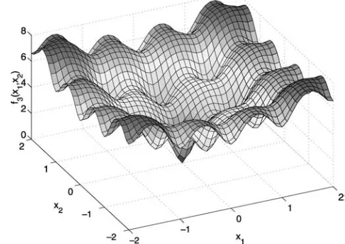
Here we present details of the test functions used in Sects. 4.1 and 4.2: the two-dimensional Branin function and thek-dimensional Modified Rosenbrock and Ackley functions (their five-dimensional variants have been used for the experiments described in this paper). They have been chosen to cover a range of complexities, with the Branin function being the simplest, the Modified Rosen-brock function having moderate multimodality, while the Ackley function featuring a high number of local optima.

Branin function

f1(x1, x2) =a(x2−bx21+cx1−d)2+e(1−f)cos(x1) +e

(A.1) wherea= 1, b= 5.1

4π2, c=

5

π, d= 6, e= 10, f= 1 8π and (x1, x2)∈[−5,10]×[0,15].

Modified Rosenbrock function

f2(x) =

1 a

_k−1

i=1

100(xi+1−x2i)2+ (1−xi)2+ k

i=1

75 sin(5(1−xi))−b

(A.2)

wherea= 206, b= 300 andx∈[−1,1]k.

Ackley’s function

f3(x) =

1 f

    −aexp

  −b

1

n

k

i=1

x2 i   −

exp

1 n

k

i=1

cos(cxi)

+a+ exp(1) +d

   

 (A.3)

Fig. 20 Branin function

wherea= 20, b= 0.2, c= 2π, d= 5.7, f= 0.8 andx∈[−2.048,2.048]k_.

Fig. 21 Two-variable version of Modified Rosenbrock’s func-tion