Efficient data structures for backtrack search SAT solvers

Efficient data structures for backtrack search SAT solvers

Inês Lynce and João Marques-Silva

IST/INESC-ID, Technical University of Lisbon, Lisbon, Portugal E-mail: {ines,jpms}@sat.inesc-id.pt

The implementation of efficient Propositional Satisfiability (SAT) solvers entails the uti-lization of highly efficient data structures, as illustrated by most of the recent state-of-the-art SAT solvers. However, it is in general hard to compare existing data structures, since different solvers are often characterized by fairly different algorithmic organizations and techniques, and by different search strategies and heuristics. This paper aims the evaluation of data struc-tures for backtrack search SAT solvers, under a common unbiased SAT framework. In addi-tion, advantages and drawbacks of each existing data structure are identified. Finally, new data structures are proposed, that are competitive with the most efficient data structures currently available, and that may be preferable for the next generation SAT solvers.

Keywords:propositional satisfiability, backtrack search

1. Introduction

In recent years Propositional Satisfiability (SAT) has successfully found a large number of significant applications. SAT has also been the subject of intensive research. New backtrack search algorithms have been proposed, that include new search strate-gies, new search techniques and new implementations. Broadly, improvements in SAT solvers have been characterized by a few significant paradigm shifts. First, GRASP [12] and rel-sat [3] very successfully proposed using clause recording and non-chronological backtracking in SAT solvers. More recently, search restart strategies have been shown to be extremely effective for solving real-world problem instances [2,8]. Finally, the most recent paradigm shift was observed first in SATO [18] and more recently and more dras-tically in Chaff [14], that proposed several significant new ideas on how to efficiently implement backtrack search SAT algorithms.

This paper proposes to further investigate the paradigm shift personified by SATO and Chaff. How effective are the data structures proposed by these SAT solvers? Are these data structures the best option for existing SAT solvers? Are these data structures the most adequate for the expected next generation SAT solvers? Is it possible to do better? This paper represents a first study to answer these questions.

then evaluated in a common SAT framework, and some of their limitations are identified and empirically characterized. The paper concludes in section 6.

2. Definitions

This section introduces the notational framework used throughout the paper. Propositional variables are denotedx1, . . . , xn, and can be assigned truth values 0 (orF)

or 1 (orT). The truth value assigned to a variablex is denoted by ν(x). (When clear from context we usex = νx, whereνx ∈ {0,1}.) A literal l is either a variable xi or

its negation¬xi. A clauseωis a disjunction of literals and a CNF formulaϕ is a

con-junction of clauses. A clause is said to besatisfied if at least one of its literals assumes value 1,unsatisfied if all of its literals assume value 0,unit if all but one literal assume value 0, andunresolved otherwise. Literals with no assigned truth value are said to be

free literals. A formula is said to be satisfied if all its clauses are satisfied, and is unsat-isfied if at least one clause is unsatunsat-isfied. The SAT problem consists of deciding whether there exists a truth assignment to the variables such that the formula becomes satisfied.

It will often be simpler to refer to clauses as sets of literals, and to the CNF formula as a set of clauses. Hence, the notationl∈ωindicates that a literallis one of the literals of clauseω, whereas the notationω ∈ϕ indicates that clauseωis one of the clauses of CNF formulaϕ.

In the following sections we shall address backtrack search algorithms for SAT. Most if not all backtrack search SAT algorithms apply extensively the unit clause rule[6]. If a clause is unit, then the sole free literal must be assigned value 1 for the for-mula to be satisfiable. In this case, the value of the literal and of the associated variable are said to beimplied. The iterated application of the unit clause rule is often referred to as Boolean Constraint Propagation (BCP) [16]. Adecision levelis associated with each variable selection and assignment. The first variable selection corresponds to decision level 1. For each new decision assignment, the decision level is incremented by 1. Vari-ables whose value is implied at a given decision level are characterized by that decision level. In general, the notationx =ν(x)@δ(x)is used to denote a variablexassigned at decision levelδ(x)with valueν(x). For implementing some of the techniques common to some of the most competitive backtrack search algorithms for SAT, it is necessary to properlyexplainthe truth assignments to the propositional variables that are implied by the clauses of the CNF formula. For example, letx =vx be a truth assignment implied

by applying the unit clause rule to a unit clause clauseω. Then the explanation for this assignment is the set of assignments associated with the remaining literals ofω, which are assigned value 0. Letω = (x1∨ ¬x2∨x3) be a clause of a CNF formulaϕ, and

assume the truth assignments {x1 = 0, x3 = 0}. Then, for the clause to be satisfied

we must necessarily havex2 = 0. We say that the implied assignment x2 = 0 has the

explanation{x1 = 0, x3 = 0}. A more formal description of explanations for implied

3. Backtrack search algorithms

Over the years a large number of algorithms has been proposed for SAT, from the original Davis–Putnam procedure [6], to recent backtrack search algorithms [3,10,12, 14,17], to local search algorithms [15], among many others.

SAT algorithms can be characterized as being eithercompleteorincomplete. Com-plete algorithms can establish unsatisfiability if given enough CPU time; incomCom-plete algorithms cannot. In a search context complete algorithms are often referred to as sys-tematic, whereas incomplete algorithms are referred to asnon-systematic.

Among the different algorithms, we believe backtrack search to be the most robust approach for solving hard, structured, real-world instances of SAT. This belief has been amply supported by extensive experimental evidence obtained in recent years [2,12,14].

3.1. General organization

The vast majority of backtrack search SAT algorithms build upon the original back-track search algorithm of Davis, Logemann and Loveland [5]. Most backback-track search SAT solvers are conceptually composed of three main stages:

1. The decision stage elects the variable and value to assign at each branching step of the search process.

2. The deduction state identifies necessary assignments as a result of each selected vari-able assignment.

3. The diagnosis stage implements the backtracking step of the algorithm.

Despite being based on the same underlying algorithm, recent backtrack search SAT al-gorithms present significant modifications, that can be categorized in terms of new search strategies, new search techniques and new implementation paradigms. In the following sections we will illustrate the most significant approaches within each category.

3.2. Search strategies

Search strategies are used to organize the search process. The most well-known search strategy is the variable branching heuristic used for selecting variables and the values to assign to them. Moreover, most of the other successful search strategies for SAT involve randomization. It is well known that randomization is essential in many local search algorithms [15]; indeed, most local search algorithms repeatedly restart the (local) search by randomly generating complete assignments. In addition, randomization has also been successfully included in variable selection heuristics of backtrack search algorithms [3]. Variable selection heuristics, by being greedy in nature, are bound to select the wrong variable at the wrong time for the wrong instance. The utilization of randomization helps reducing the probability of seeing this happening.

that different sub-trees are searched each time the search algorithm is restarted. Cur-rent state-of-the-art SAT solvers already incorporate the described forms of randomiza-tion [2,14]. In these SAT solvers variable selecrandomiza-tion heuristics are randomized and search restart strategies are utilized.

3.3. Search techniques

Besides the identification of necessary assignments using the unit-clause rule, re-ferred to as Boolean Constraint Propagation, recent state-of-the-art backtrack search SAT solvers [3,12,14,17] incorporate techniques for diagnosing conflicting conditions, thus being able to backtrack non-chronologically, and to record clauses that explain and prevent identified conflicting conditions. Clauses that are recorded due to diagnos-ing conflictdiagnos-ing conditions are referred to asconflict-induced clauses(or simplyconflict clauses). Additional techniques used in backtrack search SAT algorithms include identi-fication of unique implication points [12] and relevance-based learning [3]. (We should observe that a number of other techniques is often used as a preprocessing step [7,9].)

3.4. Implementation paradigms

Implementation issues for SAT solvers include the design of suitable data structures for storing variables, clauses and literals. The elected data structures dictate the way BCP and conflict analysis are implemented and have significant impact on the run time performance of the SAT solver. Recent state-of-the-art SAT solvers are characterized by using very efficient data structures, intended to reduce the CPU time required per each node in the search tree. Examples of efficient data structures include the head/tail lists used in SATO [17] and the watched literals used in Chaff [14].

4. Data structures for SAT

The main purposes of this section are twofold. First, to review existing SAT data structures. Second, to propose new data structures, that may be preferable for the next generation SAT solvers. Our description of SAT data structures is organized in two main categories: data structures based on adjacency lists, and lazy data structures. Moreover, we also analyze optimizations that can be applied to most data structures, by special handling of small clauses. Also, we discuss the effect of lazy data structures in accurately predicting dynamic clause size (i.e. the number of unassigned literals in a clause).

4.1. Adjacency lists

Most backtrack search SAT algorithms represent clauses as lists of literals, and associate with each variable x a list of the clauses that contain a literal inx. The lists associated with each variable can be viewed as containing the clauses that areadjacent

In the following subsections, different alternative implementations of adjacency lists are described. In each case we are interested in being able to accurately and effi-ciently identify when clauses become satisfied, unsatisfied or unit.

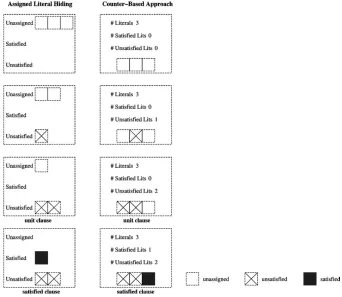
4.1.1. Assigned literal hiding

One approach to identify satisfied, unsatisfied or unit clauses consists of extracting from the clause’s list of literals all the references to unsatisfied and satisfied literals. These references are added to dedicated lists associated with each clause. As a result, satisfied clauses contain one or more literal references in the list of satisfied literals; unsatisfied clauses contain all literal references in the list of unsatisfied literals; finally, unit clauses contain one unassigned literal and all the other literal references in the list of unsatisfied literals.

This data structure is illustrated in figure 1. Whenever a literal is assigned, it is moved either to the satisfied or unsatisfied literals list. In the given example, the ternary clause is identified as unit on the third step, when only one literal is unassigned and the other two literals are unsatisfied. Observe that when the search backtracks the same operations are performed on the reverse order.

As will be shown in section 5, this organization of the adjacency list data structure is never competitive with the other approaches.

4.1.2. The counter-based approach

An alternative approach to keep track of unsatisfied, satisfied and unit clauses is to associate literal counters with each clause. These literal counters indicate how many literals are unsatisfied, satisfied and, indirectly, how many are still unassigned. A clause is unsatisfied if the unsatisfied literal counter equals the number of literals; it is satisfied if the counter of satisfied literals is greater than one; finally, it is unit if the unsatisfied literal counter equals the number of literals minus one, and there is still one unassigned literal. When a clause is declared unit, the list of literals is traversed to identify which literal needs to be assigned. An example of a SAT solver that utilizes counter-based adjacency lists is GRASP [12].

The counter-based approach is also illustrated in figure 1. Whenever a literal is given a value, either the counters for satisfied or unsatisfied literals are updated, depend-ing on the literal bedepend-ing assigned value 1 or 0, respectively. Observe that when the clause is identified as unit(#Unsatisfied Literals=#Literals−1), the whole clause is traversed in order to find the remaining unassigned literal. Moreover, counters have to be updated when the search backtracks.

4.1.3. Counter-based with satisfied clause hiding

A key drawback of using adjacency lists is that the lists of clauses associated with each variable can be large, and will grow as new clauses are recorded during the search process. Hence, each time a variable is assigned, a potentially large list of clauses needs to be traversed. Different approaches can be envisioned to overcome this drawback. For the counter-based approach of the previous section, one solution is to remove from the list of clauses of each variableallthe clauses that are known to be satisfied. Hence, each time a clauseωbecomes satisfied,ωis hidden from the list of clauses of all the variables with literals inω. The technique of hiding satisfied clauses can be traced back to the work of O. Coudert in Scherzo [4] for the Binate Covering Problem. The motivation for hiding clauses is to reduce the amount of work required each time a variable x is assigned, since in this case only the unresolved clauses associated with x need to be analyzed.

4.1.4. Satisfied clause and assigned literal hiding

One final organization of adjacency lists is to utilize the same data structures as the ones used by Scherzo [4]. In this case, unsatisfied literals get removed from literal lists in clauses, and satisfied clauses get hidden from clause lists in variables.

4.2. Lazy data structures

As mentioned in the previous section, adjacency list-based data structures share a common problem: each variablex keeps references to a potentially large number of clauses, that often increases as the search proceeds. Clearly, this impacts negatively the amount of work associated with assigningx. Moreover, it is often the case that most of x’s clause references need not be analyzed whenxis assigned, since they do not become unit or unsatisfied.

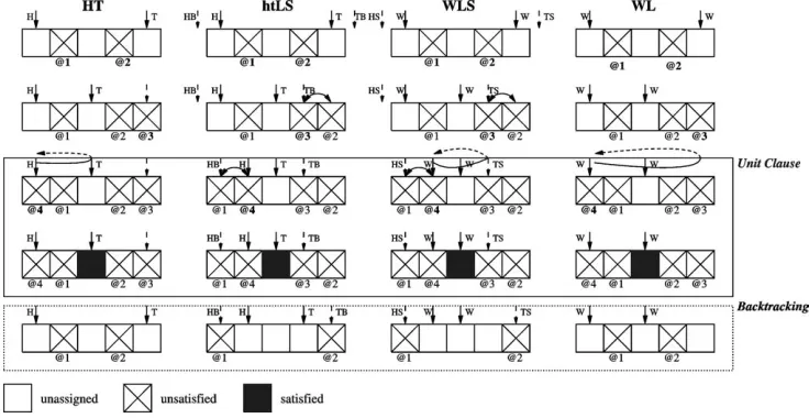
In this section we analyzelazy data structures, which are characterized by each variable keeping a reduced set of clauses’ references, for each of which the variable can be effectively used for declaring the clause as unit, as satisfied or as unsatisfied. The operation of these data structures is summarized in figure 2.

4.2.1. Sato’s head/tail lists

The first lazy data structure proposed for SAT was theHead/Tail(H/T) data ture, originally used in the SATO SAT solver [18]. As the name implies, this data struc-ture associates two references with each clause, thehead (H) and the tail (T) literal references (see figure 2). Initially the head reference points to the first literal, and the tail reference points to the last literal. Each time a literal pointed to by either the head or tail reference is assigned, a new unassigned literal is searched for. In case an unassigned literal is identified, it becomes the new head (or tail) reference, and anewreference is created and associated with the literal’s variable. In case a satisfied literal is identified, the clause is declared satisfied. In case no unassigned literal can be identified, and the other reference is reached, then the clause is declared unit, unsatisfied or satisfied, de-pending on the value of the literal pointed to by the other reference. When the search process backtracks, the references that have become associated with the head and tail

references can be discarded, and the previous head and tail references become activated (represented with a dashed arrow in figure 2 for column HT). Observe that this requires in the worst-case associating with each clause a number of literal references in variables that equals the number of literals.

4.2.2. Chaff’s watched literals

The more recent Chaff SAT solver [14] proposed a new data structure, the Watched Literals (WL), that solves some of the problems posed by H/T lists. As with H/T lists, two references are associated with each clause. However, and in contrast with H/T lists, there isnoorder relation between the two references. The lack oforderbetween the two references has the key advantage that no literal references need to be updated when backtracking takes place. In contrast, unit or unsatisfied clauses are identified only after traversingallthe clauses’ literals; a clear drawback. The identification of satisfied clauses is similar to H/T lists.

With respect to figure 2, the most significant difference between H/T lists and watched literals occurs when the search process backtracks, in which case the refer-ences to the watched literals are not modified. Moreover, and in contrast with H/T lists, for each clause the number of literal references that are associated with variables is kept

constant.

4.2.3. Head/tail lists with literal sifting

The problems identified for H/T lists and watched literals can be solved with yet another data structure, H/T lists with literal sifting (htLS). This new data structure is similar to H/T lists, but it dynamically rearranges the list of literals, ordering the clause’s assigned literals by increasing decision level. Assigned variables are sorted by non-decreasing decision level, starting from the first or last literal reference, and terminating at the most recently assigned literal references, just before the head reference and just after the tail reference. This sorting is achieved by sifting assigned literals as each is visited by the H and T literal references. The sifting is performed towards one of the ends of the literal list. The solution based on literal sifting has several advantages:

– When the clause either becomes unit or unsatisfied, there is no need to traverse all the clause’s literals to confirm this fact. Moreover, satisfied clauses are identified in the same way as for the other lazy data structures.

– As illustrated in figure 2, only four literal references need to be associated with each clause. This is in contrast with H/T lists, that in the worst-case need a number of references that equals the number of literals (even though watched literals just require two references).

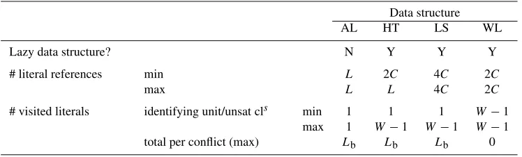
Table 1

Comparison of the data structures.

Data structure

AL HT LS WL

Lazy data structure? N Y Y Y

# literal references min L 2C 4C 2C

max L L 4C 2C

# visited literals identifying unit/unsat cls min 1 1 1 W−1 max 1 W−1 W−1 W−1 total per conflict (max) Lb Lb Lb 0 L=number of literals.

C=number of clauses.

W=number of literals in clause.

L_b=number of literals to be unassigned when backtracking.

4.2.4. Watched literals with literal sifting

One additional data structure consists of utilizing watched literals with literal sift-ing (WLS). This data structure applies literal siftsift-ing, but the references to unassigned literals are watched, in the sense that when backtracking takes place the literal refer-ences are not updated (see figure 2). This data structure keeps two watched literals, and uses two additional references for applying literal sifting and keeping assigned literals by decreasing order of decision level. Watched literals are managed as described earlier, and literal sifting is applied as proposed in the previous section.

The main advantage of the WLS data structure is the simplified backtracking process; the disadvantage is the requirement to visit all literals between the literal refer-ences HS and TS each time the clause is either unit or unsat.1

4.3. A comparison of the data structures

Besides describing the organization of each data structure, it is also interesting to characterize each one in terms of the memory requirements and computational effort. In table 1, we provide a comparison of the data structures described in the previous section. The table indicates which data structures arelazy, the (minimum and maximum) total number of literal references associated with all clauses, and also provides a broad indication of the work associated with keeping clause state when the search either moves forward (i.e. implies assignments) or backward (i.e. backtracks).

Even though it is straightforward to prove the results shown, a careful analysis of the behavior of each data structure allows establishing these results. For example, when backtracking takes place, the WL data structure updatesnoliteral references. Hence, the number of visited literal references for each conflict is 0.

1_{Observe that it is easy to reduce the number of literal references to three: two for the watched literals and}

4.4. Handling special cases: B/T clauses

As one final optimization to literal sifting, we propose the special handling of the clauses that are more common in problem instances: binary and ternary clauses. Both binary and ternary clauses can be identified as unit, sat or unsat in constant time, thus eliminating the need for moving literal references around. Since the vast majority of the initial number of clauses for most real-world problem instances are either binary or ternary, the average CPU time required to handle each clause may be noticeably reduced. In this situation, the H/T lists with literal sifting are solely applied to large clauses and to clauses recorded during the search process.

As one final comment, observe that special handling of binary/ternary clauses can also be used with all the other data structures described in this section.

4.5. Do lazy data structures suffice?

As mentioned earlier, most state-of-the-art SAT solvers currently utilize lazy data structures. Even though these data structures suffice for backtrack search SAT solvers that solely utilize Boolean Constraint Propagation, thelaziness of these data structures may pose some problems, in particular for new algorithms that aim the integration of more advanced techniques for the identification of necessary assignments, namely re-stricted resolution, two-variable equivalence, and pattern-based clause inference, among other techniques [9,13]. For these techniques, it is essential to know which clauses are binary and/or ternary. As already mentioned, lazy data structures are not capable of keep-ing precise information about the set of binary and/or ternary clauses.2 Hence, if future SAT solvers choose to integrate advanced techniques for the identification of necessary assignments, they either forgo using lazy data structures, or they apply those techniques to a subset of the total number of binary/ternary clauses. One reasonable assumption is that lazy data structures will indeed be deemed essential, and that future SAT solvers will apply advanced techniques to alazyset of binary/ternary clauses. In this situation, it becomes important to characterize thelazinessof a lazy data structure in terms of the actual number of binary/ternary clauses it is capable of identifying. A data structure that is able to identify the largest number of binary/ternary clauses is clearly the best option for the implementation of advanced search techniques.

5. Experimental results

This section evaluates the different SAT data structures described in the previous section. We start by introducing the algorithmic framework used for the experimental evaluation, JQUEST. The next step is to analyze the results of using different data struc-tures in SAT solvers. Finally, we also evaluate the accuracy of lazy SAT data strucstruc-tures in estimating the number of satisfied, binary and ternary clauses.

2_{Clearly, this can be done by associating additional literal references with each clause, and as a result by}

5.1. The JQUEST SAT framework

In order to experimentally evaluate the different data structures described in the previous section, in a controlled experiment that ensures that only the differences in data structures are evaluated, a dedicated SAT solving framework is needed. Besides differing data structures and coding styles, each existing SAT solver implements its own set of search techniques, strategies and heuristics. Hence, a comparison between state-of-the-art SAT solvers hardly guarantees meaningful results with respect to the underlying data structures.

In order to experimentally evaluate the different algorithms, in a controlled exper-iment that ensures that only specific differences are evaluated, a dedicated SAT solving framework is needed. Consequently, we developed the JQUEST SAT framework, a Java implementation that can be used to conduct unbiased experimental evaluations of SAT algorithms and techniques.

As a result we developed the JQUEST SAT framework, a Java implementation that can be used to conduct unbiased experimental evaluations of SAT algorithms and tech-niques. For a given problem instance and for each data structure considered, JQUEST guarantees thesamealgorithmic organization and enforces thesamesearch tree.

Even though Java yields a necessarily slower implementation, it is also plain that it allows fast prototyping of new algorithms. Moreover, well-devised Java implemen-tations can be used as the blueprint for faster C/C++ implemenimplemen-tations. In the case of JQUEST, all the proven strategies and techniques for SAT have been implemented: clause recording; non-chronological backtracking; search restarts; random backtracking; and also variable selection heuristics.

For the results shown below a P-III@833 MHz Linux Red Hat 6.1 machine with 1 GByte of physical memory was used. The Java Virtual Machine used was SUN’s HotSpot JVM for JDK1.3.

5.2. Lazy vs. non-lazy data structures

In order to compare the different data structures, the following algorithm organiza-tion of JQUEST is used:

– The VSIDS (Variable State Independent Decaying Sum) [14] heuristic is used for all data structures. Our implementation of the VSIDS heuristic closely follows the one proposed in Chaff.

– Identification of necessary assignments solely uses boolean constraint propagation. We should note that, in order to guarantee that the same search tree is visited, the unit clauses are handled in afixed pre-definedorder.

– Conflict analysis is implemented as in GRASP. However, only a single clause is recorded (by stopping at the first Unique Implication Point (UIP) [12] as suggested by the authors of Chaff [14]). Moreover,noclauses are ever deleted.

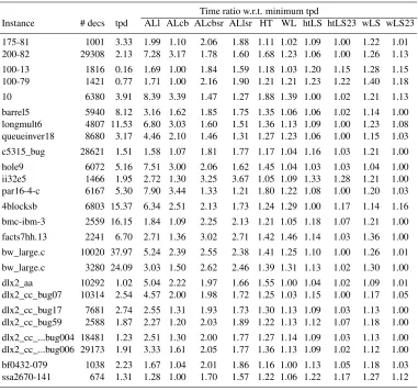
Table 2

Results for the time per decision (tpd, in msec). Time ratio w.r.t. minimum tpd

Instance # decs tpd ALl ALcb ALcbsr ALlsr HT WL htLS htLS23 wLS wLS23 175-81 1001 3.33 1.99 1.10 2.06 1.88 1.11 1.02 1.09 1.00 1.22 1.01 200-82 29308 2.13 7.28 3.17 1.78 1.60 1.68 1.23 1.06 1.00 1.26 1.13 100-13 1816 0.16 1.69 1.00 1.84 1.59 1.18 1.03 1.20 1.15 1.28 1.15 100-79 1421 0.77 1.71 1.00 2.16 1.90 1.21 1.21 1.23 1.22 1.40 1.18 10 6380 3.91 8.39 3.39 1.47 1.27 1.88 1.39 1.00 1.02 1.21 1.13 barrel5 5940 8.12 3.16 1.62 1.85 1.75 1.35 1.06 1.06 1.02 1.14 1.00 longmult6 4807 11.53 6.80 3.03 1.60 1.51 1.36 1.13 1.09 1.00 1.23 1.08 queueinver18 8680 3.17 4.46 2.10 1.46 1.31 1.27 1.23 1.06 1.00 1.15 1.03 c5315_bug 28621 1.51 1.58 1.07 1.81 1.77 1.17 1.04 1.16 1.03 1.21 1.00 hole9 6072 5.16 7.51 3.00 2.06 1.62 1.45 1.04 1.03 1.03 1.04 1.00 ii32e5 1466 1.95 2.72 1.30 3.25 3.67 1.05 1.09 1.33 1.28 1.21 1.00 par16-4-c 6167 5.30 7.90 3.44 1.33 1.21 1.80 1.22 1.08 1.00 1.20 1.03 4blocksb 6803 15.37 6.34 2.51 2.13 1.73 1.24 1.29 1.00 1.17 1.14 1.16 bmc-ibm-3 2559 16.15 1.84 1.09 2.25 2.13 1.21 1.05 1.18 1.07 1.21 1.00 facts7hh.13 2241 6.70 2.71 1.36 3.02 2.71 1.42 1.46 1.14 1.03 1.36 1.00 bw_large.c 10020 37.97 5.24 2.39 2.55 2.38 1.41 1.25 1.10 1.00 1.26 1.01 bw_large.c 3280 24.09 3.03 1.50 2.62 2.46 1.39 1.31 1.13 1.02 1.30 1.00 dlx2_aa 10292 1.02 5.04 2.22 1.97 1.66 1.55 1.00 1.04 1.02 1.09 1.01 dlx2_cc_bug07 10314 2.54 4.57 2.00 1.98 1.72 1.25 1.03 1.15 1.00 1.17 1.05 dlx2_cc_bug17 7681 2.74 2.55 1.31 1.93 1.73 1.30 1.13 1.09 1.03 1.13 1.00 dlx2_cc_bug59 2588 1.87 2.27 1.20 2.03 1.89 1.22 1.13 1.12 1.07 1.18 1.00 dlx2_cc_...bug004 18481 1.23 2.51 1.30 2.00 1.77 1.27 1.14 1.09 1.03 1.13 1.00 dlx2_cc_...bug006 29173 1.91 3.33 1.61 2.05 1.77 1.36 1.13 1.09 1.02 1.12 1.00 bf0432-079 1038 2.23 1.67 1.04 2.01 1.86 1.16 1.00 1.13 1.05 1.18 1.03 ssa2670-141 674 1.31 1.28 1.00 1.70 1.57 1.22 1.06 1.22 1.17 1.27 1.12

The results of comparing the different data structures are shown in table 2. In order to perform this comparison, instances were selected from several classes of instances. In all cases, the problem instances chosen are solved with several thousand decisions, usually taking a few tens of seconds. Hence, the instances chosen are significantly hard, but can be solved without sophisticated search strategies, that would not necessarily guarantee the same search tree for all data structures considered.

de-Figure 3. Analysis of performance.

notes H/T lists; WL denotes watched literals; htLS denotes H/T lists with literal sifting; finally, htLS23 denotes H/T lists with literal sifting and with special handling of binary and ternary clauses.

From the table of results, several conclusions can be drawn. Clearly, lazy data structures are in general significantly more efficient that data structures based on ad-jacency lists. Regarding the data structures based on adad-jacency lists, the utilization of satisfied clause and assigned literal hiding does not pay off. For the lazy data structures, H/T lists are in general significantly slower than either watched literals or H/T lists with literal sifting. Finally, H/T lists with literal sifting tend to be somewhat more efficient than watched literals. This results in part from the literal sifting technique, that allows literals assigned at low decision levels not to be repeatedly analyzed during the search process.

Despite the previous results that indicate H/T lists with literal sifting to be in gen-eral faster than the watched litgen-erals data structure, one may expect the small performance difference between the two data structures to be eliminated by careful C/C++ implemen-tations. This is justified by the expected better cache behavior of watched literals [14].

A summary of the experimental results for a selected number of data structures is shown in figure 3. The graph represents the number of instances that to be solved require less than a given time ratio wrt the time per decision. As can be observed, both the htLS and WL data structures are in the vast majority of cases very close to time ratio 1.

5.3. Limitations of lazy data structures

two-variable equivalence conditions (from pairs of binary clauses), restricted resolution (be-tween binary and ternary clauses), and pattern-based clause inference conditions (also using binary and ternary clauses) [1,9,13]. Even though some of these techniques are often used as a preprocessing step by SAT solvers, their application during the search phase has been proposed in the past [11,13]. The objective of this section is thus to measure the laziness of lazy data structures during the search process. The more lazy a (lazy) data structure is, the less suitable it is for implementing (lazy) advanced rea-soning techniques during the search process. As we show below, no lazy data structure provides completely accurate information regarding the number of binary, ternary or sat-isfied clauses. However, some lazy data structures are significantly more accurate than others. Hence, if some form oflazyimplementation of advanced SAT techniques is to be used during the search process, some lazy data structures are significantly more adequate than others.

We start by observing that the watched literals data structure is unable to dynam-ically identify binary and ternary clauses, since there is no order relation between the two references used. Identifying binary and ternary clauses would involve maintaining additional information than what is required by the watched literals data structure.3

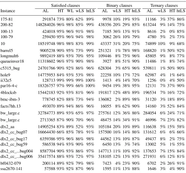
Table 3 includes results measuring the accuracy of each lazy data structure in iden-tifying satisfied, binary and ternary clauses among recorded clauses. The reference val-ues considered are given by the valval-ues obtained with adjacency lists data structures, which are the actual exact values. (Observe that, as mentioned above, the watched lit-erals data structure can only be used for identifying satisfied clauses.) From the results shown, we can conclude that H/T lists with literal sifting provide by far the most accurate estimates of the number of satisfied, binary and ternary clauses. In addition, for satisfied and binary clauses, the measured accuracy is often close to the maximum possible value, whereas for ternary clauses the accuracy values tend to be somewhat lower.

6. Conclusions

This paper surveys existing data structures for backtrack search SAT algorithms and proposes new data structures. In addition, we introduce the JQUEST SAT frame-work, that allows the fast prototyping of SAT solvers, and can be used for the unbiased evaluation of SAT data structures and algorithms. The JQUEST SAT framework is also expected to serve as the blueprint for the implementation of efficient SAT algorithms in C/C++.

Regarding the evaluation of SAT data structures, the experimental results, indicate that some of the new data structures proposed may be preferable for the next generation

3_{Observe that the utilization of two references only guarantees the identification of unit clauses. The lack}

Table 3

Results for the accuracy of recorded clause identification.

Satisfied clauses Binary clauses Ternary clauses Instance AL HT WL wLS htLS AL wLS HT htLS AL wLS HT htLS 175-81 291874 73% 80% 62% 89% 9978 10% 19% 93% 11166 3% 37% 86% 200-82 148284026 96% 98% 85% 99% 438356 20% 29% 85% 613244 9% 14% 75% 100-13 424018 95% 96% 91% 98% 7185 36% 13% 91% 8616 2% 0% 85% 100-79 259450 95% 96% 94% 98% 3062 26% 10% 79% 4780 5% 2% 73% 10 18519748 98% 98% 83% 99% 43337 31% 20% 75% 74899 10% 9% 68% barrel5 9005238 90% 95% 73% 99% 251321 1% 78% 98% 168820 1% 50% 92% longmult6 9892419 88% 93% 70% 95% 109446 8% 75% 96% 45805 9% 8% 77% queueinver18 11318602 96% 97% 90% 98% 3927 8% 51% 90% 11486 1% 8% 74% c5315_bug 24701766 90% 92% 86% 96% 628304 3% 65% 96% 539811 1% 50% 90% hole9 14775953 84% 93% 53% 98% 22258 10% 17% 72% 62987 4% 1% 64% ii32e5 128713 99% 99% 99% 100% 1413 4% 14% 70% 1256 0% 4% 50% par16-4-c 18326757 97% 99% 66% 100% 9454 19% 38% 95% 12131 7% 37% 90% 4blocksb 15442183 92% 93% 81% 96% 191817 12% 48% 89% 196534 7% 16% 72% bmc-ibm-3 778745 82% 88% 73% 94% 136082 2% 89% 98% 31120 3% 18% 89% facts7hh.13 493070 89% 94% 86% 96% 16055 8% 62% 90% 14160 3% 52% 84% bw_large.c 32784773 89% 93% 65% 97% 275761 12% 36% 86% 284054 6% 24% 71% bw_large.c 2713365 87% 90% 70% 96% 48475 14% 34% 91% 46996 7% 23% 82% dlx2_aa 14905254 83% 89% 52% 93% 105184 20% 10% 89% 116638 5% 15% 58% dlx2_cc_bug07 16664430 66% 85% 78% 91% 157500 16% 14% 86% 131612 6% 6% 66% dlx2_cc_bug17 6359386 95% 96% 86% 98% 44562 13% 10% 87% 49437 8% 2% 75% dlx2_cc_bug59 586538 94% 93% 90% 95% 6450 13% 3% 74% 13002 5% 1% 55% dlx2_cc_...bug004 8587704 90% 93% 86% 97% 147713 11% 10% 92% 137653 7% 15% 84% dlx2_cc_...bug006 35417574 88% 93% 72% 97% 318105 12% 13% 93% 271931 6% 12% 81% bf0432-079 200114 89% 92% 79% 98% 7423 4% 23% 90% 6702 2% 26% 91% ssa2670-141 57588 93% 92% 87% 96% 1595 11% 13% 88% 1646 3% 4% 90%

SAT solvers. This conclusion results from these new data structures being in general faster, but mostly due to coping better with the laziness of recent (lazy) data structures.

Related research work involves evaluating how advanced SAT techniques perform with lazy structures. Clearly, this will depend on the accuracy of each data structure to identify binary/ternary clauses. As a result, data structures that are unable to gather the information required by advanced SAT techniques may be inadequate for the next generation state-of-the-art SAT solvers.

Acknowledgements

References

[1] F. Bacchus, Exploiting the computational tradeoff of more reasoning and less searching, in: Pro-ceedings of Fifth International Symposium on Theory and Applications of Satisfiability Testing(2002) pp. 7–16.

[2] L. Baptista and J.P. Marques-Silva, Using randomization and learning to solve hard real-world in-stances of satisfiability, in: International Conference on Principles and Practice of Constraint Pro-gramming, ed. R. Dechter, Lecture Notes in Computer Science, Vol. 1894 (2000) pp. 489–494. [3] R. Bayardo, Jr. and R. Schrag, Using CSP look-back techniques to solve real-world SAT instances,

in:Proceedings of the National Conference on Artificial Intelligence(1997) pp. 203–208.

[4] O. Coudert, On solving covering problems, in: Proceedings of the ACM/IEEE Design Automation Conference(1996) pp. 197–202.

[5] M. Davis, G. Logemann and D. Loveland, A machine program for theorem-proving, Communications of the Association for Computing Machinery 5 (1996) 394–397.

[6] M. Davis and H. Putnam, A computing procedure for quantification theory, Journal of the Association for Computing Machinery 7 (1960) 201–215.

[7] A.V. Gelder and Y.K. Tsuji, Satisfiability testing with more reasoning and less guessing, in: Second DIMACS Implementation Challenge, eds. D.S. Johnson and M.A. Trick (American Mathematical Society, 1993).

[8] C.P. Gomes, B. Selman and H. Kautz, Boosting combinatorial search through randomization, in: Proceedings of the National Conference on Artificial Intelligence(1998) pp. 431–437.

[9] J.F. Groote and J.P. Warners, The propositional formula Checker Heerhugo, in:Proceedings of SAT 2000, eds. I. Gent, H. van Maaren and T. Walsh (IOS Press, 2000) pp. 261–281.

[10] C.M. Li and Anbulagan, Look-ahead versus look-back for satisfiability problems, in:Proceedings of the International Conference on Principles and Practice of Constraint Programming(1997) pp. 341– 355.

[11] J.P. Marques-Silva, Algebraic simplification techniques for propositional satisfiability, in: Interna-tional Conference on Principles and Practice of Constraint Programming, ed. R. Dechter, Lecture Notes in Computer Science, Vol. 1894 (2000) pp. 537–542.

[12] J.P. Marques-Silva and K.A. Sakallah, GRASP: A new search algorithm for satisfiability, in: Proceed-ings of the ACM/IEEE International Conference on Computer-Aided Design(1996) pp. 220–227. [13] J.P. Marques-Silva and K.A. Sakallah Boolean satisfiability in electronic design automation, in:

Pro-ceedings of the ACM/IEEE Design Automation Conference(2000) pp. 675–680.

[14] N. Moskewicz, C. Madigan, Y. Zhao, L. Zhang and S. Malik, Engineering an efficient SAT solver, in: Proceedings of the Design Automation Conference(2001) pp. 530–535.

[15] B. Selman and H. Kautz, Domain-independent extensions to GSAT: Solving large structured satisfia-bility problems, in:Proceedings of the International Joint Conference on Artificial Intelligence(1993) pp. 290–295.

[16] R. Zabih and D.A. McAllester, A rearrangement search strategy for determining propositional satisfi-ability, in:Proceedings of the National Conference on Artificial Intelligence(1988) pp. 155–160. [17] H. Zhang, SATO: An efficient propositional prover, in:Proceedings of the International Conference

on Automated Deduction(1997) pp. 272–275.