A Linear Algebraic Technique with an Application in Semantic Image Retrieval

Application in Semantic Image Retrieval

Jonathon S. Hare1_{, Paul H. Lewis}1_, Peter G.B. Enser2_{, and Christine J. Sandom}2

1 _{School of Electronics and Computer Science, University of Southampton, UK}

{jsh2, phl_}@ecs.soton.ac.uk

2 _{School of Computing, Mathematical and Information Sciences,}

University of Brighton, UK {p.g.b.enser, c.sandom}@bton.ac.uk

Abstract. This paper presents a novel technique for learning the under-lying structure that links visual observations with semantics. The tech-nique, inspired by a text-retrieval technique known as cross-language latent semantic indexing uses linear algebra to learn the semantic struc-ture linking image feastruc-tures and keywords from a training set of annotated images. This structure can then be applied to unannotated images, thus providing the ability to search the unannotated images based on

key-word. Thisfactorisation approach is shown to perform well, even when

using only simple global image features.

1 Introduction

Automatic annotation of images has come to the fore as a means of trying to achieve the integration of content-based and text-based image retrieval. An overview of the techniques which have been used in auto-annotation has been provided by Hare et al [1], and we are currently exploring how such techniques can meet the real needs of image searchers in limited domains. This work is being undertaken within the Bridging the Semantic Gap Project, as described by Enser et al [2].

In this paper, we propose a linear algebraic method forlearning the semantic structure between terms in an annotated training set of images. Unannotated images can then be projected into the structure. The resulting space is unique in that it allows images to be ranked on their relevance to terms that may not have been explicitly assigned to the images, even though the image is relevant to the term.

2 Using Linear-Algebra to Associate Images and Terms

Latent Semantic Indexing (LSI) [3] is a technique in text-retrieval for index-ing documents in a dimensionally-reduced semantic vector space. Landauer and Littman [4], demonstrate a system based on LSI for performing text searching

H. Sundaram et al. (Eds.): CIVR 2006, LNCS 4071, pp. 31–40, 2006. c

on a set of French and English documents where the queries could be in either French or English (or conceivably both), and the system would return documents in both languages which corresponded to the query. Landauer’s system negated the need for explicit translations of all the English documents into French; in-stead, the system was trained on a set of English documents and versions of the documents translated into French, and through a process called ‘folding-in’, the remaining English documents were indexed without the need for explicit translations. This idea has become known asCross-Language Latent Semantic Indexing (CL-LSI).

Monay and Gatica-Perez [5] attempted to use straight LSI with simple domain vectors for auto-annotation. They first created a training matrix of cross-domain vectors and applied LSI. By querying the left-hand subspace they were able to rank an un-annotated query document against each annotation term in order to assess likely annotations to apply to the image.

Our approach, based on a generalisation of CL-LSI, is different because we do not explicitly annotate images. The technique works by placing unannotated images in a semantic-space which can be queried by keyword.

In general, any document (be it text, image, or even video) can be described by a series of observations, or measurements, made about its content. We re-fer to each of these observations as terms. Terms describing a document can be arranged in a vector of term occurrences, i.e. a vector whosei-th element contains

a count of the number of times thei-th term occurs in the document. There is

nothing stopping a term vector having terms from a number of different modal-ities. For example a term vector could contain term-occurrence information for both ‘visual’ terms and textual annotation terms.

Given a corpus ofndocuments, it is possible to form a matrix ofm

observa-tions or measurements (i.e. a term-document matrix). This m_×n observation

matrix, O, essentially represents a combination of terms and documents, and can be factored into a separate term matrix,T, and document matrix,D:

O=TD . (1)

These two matrices can be seen to represent the structure of a semantic-space co-inhabited by both terms and documents. Similar documents and/or terms in this space share similar locations. The advantage of this approach is that it doesn’t requirea-priori knowledge and makes no assumptions of either the relationships between terms or documents. The primary tool in this factorisation is the Singular Value Decomposition. This factorisation approach to decomposing a measurement matrix has been used before in computer vision; for example, in factoring 3D-shape and motion from measurements of tracked 2D points using a technique known as Tomasi-Kanade Factorisation [6].

indexed. These documents need not be fully observed; for example, they may consist of only ‘visual’ terms. Any unobserved terms are represented by zeros. The document-space of this second observation matrix is then created using the term matrix from the first stage as a basis. The idea behind this is that any term-term relationships that were uncovered in the training stage will be applied to the test data, thus giving the test datapseudo-values for the unobserved terms. The net result is that we are left with a new document-space which can be searched by any of the terms used in the training set, even if they were not directly observed in the test set.

2.1 Decomposing the Observation Matrix

Following the reasoning of Tomasi and Kanade [6], although modified to fit measurements of terms in documents, we first show how the observation matrix can be decomposed into separate term and document matrices.

Lemma 1 (The rank principle for a noise-free term-document matrix).

Without noise, the observation matrix,O, has a rank at most equal to the number of independent terms or documents observed.

The rank principle expresses the simple fact that if all of the observed terms are independent, then the rank of the observation matrix would be equal to the number of terms,m. In practice, however, terms are often highly dependent

on each other, and the rank is much less than m. Even terms from different

modalities may be interdependent; for example a term representing the colour

red, and the word “Red”. This fact is what we intend to exploit.

In reality, the observation term-document matrix is not at all noise free. The observation matrix,O can be decomposed using SVD into am×rmatrix U,

a r×r diagonal matrix Σ and a r×n matrix VT_{, O = UΣV}T

, such that

UT_{U =VV}T _{= V}T_{V =I, where I is the identity matrix. Now partitioning}

theU, ΣandVT _{matrices as follows:}

U=!Uk UN" }m,

#$%&

k #$%&r−k

Σ='Σk 0

0 ΣN

( }k

}r−k,

#$%&

k #$%&r−k

VT ₌

'_VT k

VT N

( }k

}r−k ,

#$%&

n

(2)

we have,UΣVT _=U

kΣkVTk +UNΣNVTN.

Assume O∗ _{is the ideal, noise-free observation matrix, with k independent}

terms. The rank principle implies that the singular values of O∗ _{are at most} k. Since the singular values of Σ are in monotonically decreasing order, Σk

must contain all of the singular values ofO∗_{. The consequence of this is that}

UNΣNVTN must be entirely due to noise, and UkΣkVTk is the best possible

approximation toO∗_.

Lemma 2 (The rank principle for a noisy term-document matrix).All of the information about the terms and documents inOis encoded in itsklargest

We now define the estimated noise-free term matrix,Tˆ, and document matrix, ˆ

D, to be Tˆ def= Uk, and,Dˆ def= ΣkVTk, respectively. From Equation 1, we can

write

ˆ

O=T ˆˆD, (3)

whereOˆ represents the estimated noise-free observation matrix.

Interpreting the Decomposition. The two vector bases created in the de-composition form an aligned vector-space of terms and documents. The rows of the term matrix create a basis representing a position in the space of each of the observed terms. The columns of the document matrix represent positions of the observed documents in the space. Similar documents and terms share similar locations in the space.

2.2 Using the Terms as a Basis for New Documents

Theorem 1 (Projection of partially observed measurements). The term-matrix of a decomposed fully-observed measurement matrix can be used to project a partially observed measurement matrix into a document matrix that encapsulates estimates of the unobserved terms.

Manipulating Equation 3 gives us a method of projecting a partially-observed observation matrix,P into the basis created by the term matrix, Tˆ. The un-derlying assumption is that if we were to project the original fully-observed observation matrix (i.e.P=Oˆ), then we should get the same document basis.

P=T ˆˆD

∴Dˆ =Tˆ−1_P=TˆT_Tˆˆ_T−1_P=TˆT_{P (4)}

Therefore, to project a new partially observed measurement matrix into a basis created from a fully observed training matrix, we need only pre-multiply the new observation matrix by the transpose of the training term matrix. The columns of this new document matrix represent the locations in the semantic space of the documents. In order to query the document set for documents relevant to a term, we just need to rank all of the documents based on their position in the space with respect to the position of the query term in the space. The cosine similarity is a suitable measure for this task.

Thus far, we have ignored the value of k. The rank principle states that k

is such that all of the semantic structure of the observation matrix, minus the noise is encoded in the singular values and eigenvectors.kis also the number of

independent, un-correlated terms in the observation matrix. In practice,k will

vary across data-sets, and so we have to estimate its value empirically.

3 Experimental Results

in these data-sets have ground truth annotations, it is possible to automatically assess the performance of the retrieval. By splitting the data-sets into a training set and testing set, it is possible to attempt retrieval for each of the keyword terms and mark test images as relevant if they contained the query term in their annotations. Results from this technique are presented against results using the

hard annotations from the vector-space propagation technique described in [9].

3.1 Experiments with the Washington Data-Set and SIFT ‘Visual’ Terms

We split the Washington data-set [7] into a training set of 349 images, and a test set of 348 images. Each of the images was indexed using ‘visual’ terms from quantised local SIFT descriptors about interest points picked from peaks in a difference-of-Gaussian pyramid [9, 10]. The size of the visual vocabulary was fixed to 3000 terms [10].

Choosing a Good Value fork. In order to select a value fork, we need to try

and optimise the retrieval. A good statistic of overall retrieval performance is the Mean Average Precision (MAP). Plots of the average precision versus varying values ofkfor four different queries in the test set are shown in Figure 1. A plot

of the MAP over all possible queries in the training set, is shown in Figure 2. Figure 1 shows that there is a very large amount of variation of average precision across different queries. This is in a large part due to biases in both the training set of images and in the test set. For example, both the training set and test set contain an approximately equal number of images of a football stadium, however, the number ofstadiumimages in the training set is quite large in comparison to many of the other queries. The net effect is that the “Stadium” query is particularly well trained. Well trained queries can also result from few training images when the training image is sufficiently visually dissimilar to the other images (i.e. it contains a fairly unique combination of visual terms).

Unfortunately, Figure 2 doesn’t show a peak from which to select a good value ofk, instead it is asymptotic to a mean average precision of about 0.38. However,

given the constraint that we want to chooseksuch that it is the smallest it can

be whilst still giving good retrieval, we chose a value ofk= 100 for the following

experiments.

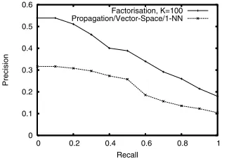
Overall Retrieval Effectiveness. The overall retrieval effectiveness of the technique is characterised in Figure 3. As can be seen, the factorisation approach outperforms the propagation approach at all values of recall.

The precision-recall curves in Figure 3 don’t truly reflect the whole perfor-mance of the approach because certain queries are better performing than others. Figure 5 illustrates this by showing the average precision for each of the queries, sorted by decreasing precision. For clarity, only queries yielding an average pre-cision of above 0.5 are shown.

0 0.2 0.4 0.6 0.8 1 1.2

0 50 100 150 200 250 300 350

Average Precision k Bridge Stadium Mountain Tree

Fig. 1.The effect of k on average preci-sion for four different queries

0 0.1 0.2 0.3 0.4 0.5

0 50 100 150 200 250 300 350

Mean Average Precision

k

All Queries Average

Fig. 2. The effect of k on the Mean-Average Precision over all queries

0 0.1 0.2 0.3 0.4 0.5 0.6

0 0.2 0.4 0.6 0.8 1

Precision

Recall Factorisation, K=100 Propagation/Vector-Space/1-NN

Fig. 3.Average precision-recall curves for the different algorithms over all queries

0 0.2 0.4 0.6 0.8 1 1.2

0 0.2 0.4 0.6 0.8 1

Precision Recall Propagation/Vector-Space/1-NN Factor., K=150 Factor., K=100 Factor., K=50

Fig. 4.Precision-Recall curves for query-ing with the keyword “Bridge”

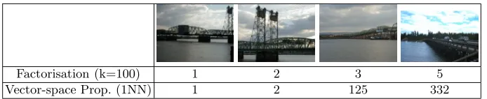
There are ten occurrences of the annotation keyword “Bridge” in the Washington data-set. Of these ten occurrences, four images are in the test set and six in the training set. One of the training images has been labelled with “Bridge”, although it doesn’t actually appear to contain a bridge. This mislabelling of images corresponds to noise, and the algorithms need to be robust to noise within the data-set. The training images are shown in Figure 6. Figure 4 illustrates the effect on precision over different recall values using both the Factorisation algorithm and the vector-space propagation algorithm. Three different values of

k for the factorisation algorithm are shown in the figure. The precision recall

curves show that both of the algorithms exhibit perfect precision up to recall values of 0.5, but then tend to drop off.

Pompoms

Corals

Rowboat Fountain Stadium Stand

Football Field

Banner

Horn Instruments

Track _Bridge Struct Barge

Cobblestones

Band Tree

Red Square Ferryboat Flower _Building

Cheerleader

Line Post _Snow

Clay Houses

Water Mast _Stands Arch Bush

Leafless Tree Cloudy Sky Overcast Sky Kangaroo Geyser Flying Fox

MAP

0.0 0.2 0.4 0.6 0.8 1.0

Fig. 5. Average precision of all queries with precision > 0.5, sorted by decreasing precision

Fig. 6.Training images containing the “Bridge” keyword

3.2 The Corel Data-Set

In the previous subsection we proposed using SIFT visual terms to model the image content. However, this is not the only option; the observation matrix could conceivably contain observations of any type of feature. In order to demonstrate the power of the factorisation technique, we use a much simpler feature; a 64-bin global RGB histogram. We use the training set of 4500 images and test set of 500 images from the Corel data-set described in [8].

Following the methodology for optimising k based on MAP described

previ-ously, we setk= 43. Overall averaged precision-recall curves of the factorisation

and propagation approaches are shown in Figure 8. As before, the factorisation approach outperforms the propagation approach. Whilst the overall averaged precision-recall curve doesn’t achieve a very high recall and falls off fairly rapidly, this isn’t indicative of all the queries; some query terms perform much better than others. Figure 9 shows precision-recall curves for some queries with good

performance.

Ideally, we would like to be able to perform a direct comparison between our factorisation method and the results of the statistical machine-translation (MT)

Factorisation (k=100) 1 2 3 5

Vector-space Prop. (1NN) 1 2 125 332

0 0.05 0.1 0.15 0.2

0 0.2 0.4 0.6 0.8 1

Precision

Recall Factorisation, K=43 Propagation/RGBHist/1-NN

Fig. 8.Average Precision-Recall plots for the Corel data-set using RGB-Histogram descriptors for both the factorisation and propagation algorithms

0 0.2 0.4 0.6 0.8 1 1.2

0 0.2 0.4 0.6 0.8 1

Precision

Recall needles

whales sun jet roofs cave snow

Fig. 9.Precision-Recall curves for the top seven Corel queries using factorisation

(k= 43)

model presented by Duygulu et al [8], which has become a benchmark against which many auto-annotation systems have been tested. Duygulu et al present their precision and recall values as single points for each query, based on the number of times the query term was predicted throughout the whole test set. In order to compare results it should be fair to compare the precision of the two methods at the recall given in the MT results. Table 1 summarises the results over the 15best queries found by the MT system (base results), corresponding to recall values greater than 0.4.

Table 1 shows that nine of of the fifteen queries had better precision for the same value of recall with the Factorisation algorithm. This higher precision at

Table 1.Comparison of precision values for equal values of recall between the machine translation model [8] and the factorisation approach

Query Word Recall Precision

Machine Translation Factorisation,

Base Results, th=0 RGB Histogram, K=43

petals 0.50 1.00 0.13

sky 0.83 0.34 0.35

flowers 0.67 0.21 0.26

horses 0.58 0.27 0.24

foals 0.56 0.29 0.17

mare 0.78 0.23 0.19

tree 0.77 0.20 0.24

people 0.74 0.22 0.29

water 0.74 0.24 0.34

sun 0.70 0.28 0.52

bear 0.59 0.20 0.11

stone 0.48 0.18 0.22

buildings 0.48 0.17 0.25

the same recall can be interpreted as saying that more relevant images are re-trieved with the factorisation algorithm for the same number of images rere-trieved as with the machine learning approach. This result even holds for Duygulu et al’s slightly improvedretrained result set. This implies, somewhat surprisingly, that even by just using the rather simple RGB Histogram to form the visual observa-tions, the factorisation approach performs better than the machine translation approach for a number of queries. This, however does say something about the relative simplicity of the Corel dataset [11]. Because not all of the top perform-ing results from the factorisation approach are reflected in thebest results from the machine translation approach, it follows that the factorisation approach may actually perform better on a majority ofgood queries compared to the machine translation model.

4 Conclusions and Future Work

This paper presented a novel approach to building a semantic space for image retrieval using a linear algebraic factorisation. Performance of the technique is good, even when using a simple global image feature such as the RGB histogram. The approach is exciting because it models the semantic gap between image descriptors and keywords in a flexible way. The factorisation technique does not produce equal performance for all queries. The reasons for this are most likely two-fold; firstly, the visual features used to represent the image may not have been sufficient to represent the keyword. Secondly, the training data may not have been sufficient to learn a good representation for the term. In terms of the Corel data-set using RGB histogram features, the factorisation approach works particularly well with annotations that can be described globally across the image by colour alone. For example, searching for ‘sun’ returns images with many warm yellow tones, and searching for ‘snow’ returns images with lots of white colours.

More experimentation needs to be performed to investigate the performance of the factorisation approach. In particular, it would be interesting to use the image descriptors created by [8] to build our observation matrix, and then to directly compare retrieval results with other automatic annotation approaches. It would also be interesting to investigate the scalability of the approach.

In the ‘Bridging the semantic gap’ project, we aim to test this approach more extensively with picture librarians, in an attempt to establish its ability as a system offering the potential of semantic search.

Acknowledgements

References

[1] Hare, J.S., Lewis, P.H., Enser, P.G.B., Sandom, C.J.: Mind the gap. In Chang, E.Y., Hanjalic, A., Sebe, N., eds.: Multimedia Content Analysis, Management, and Retrieval 2006. Volume 6073., San Jose, California, USA, SPIE (2006) 607309–1– 607309–12

[2] Enser, P.G.B., Sandom, C.J., Lewis, P.H.: Surveying the reality of semantic image retrieval. In Bres, S., Laurini, R., eds.: VISUAL 2005. Volume 3736 of LNCS., Amsterdam, Netherlands, Springer (2005) 177–188

[3] Deerwester, S.C., Dumais, S.T., Landauer, T.K., Furnas, G.W., Harshman, R.A.: Indexing by latent semantic analysis. Journal of the American Society of

Infor-mation Science41(1990) 391–407

[4] Landauer, T.K., Littman, M.L.: Fully automatic cross-language document

retrieval using latent semantic indexing. In: Proceedings of the Sixth Annual Conference of the UW Centre for the New Oxford English Dictionary and Text Research, Waterloo, Ontario, Canada (1990) 31–38

[5] Monay, F., Gatica-Perez, D.: On image auto-annotation with latent space models. In: MULTIMEDIA ’03: Proceedings of the eleventh ACM international conference on Multimedia, ACM Press (2003) 275–278

[6] Tomasi, C., Kanade, T.: Shape and motion from image streams under

orthogra-phy: a factorization method. IJCV 9(1992) 137–154

[7] University of Washington: Ground truth image database. http://www.cs.

washington.edu/research/imagedatabase/groundtruth/ (2004)

[8] Duygulu, P., Barnard, K., de Freitas, J.F.G., Forsyth, D.A.: Object recognition as machine translation: Learning a lexicon for a fixed image vocabulary. In: ECCV ’02: Proceedings of the 7th European Conference on Computer Vision-Part IV, London, UK, Springer-Verlag (2002) 97–112

[9] Hare, J.S., Lewis, P.H.: Saliency-based models of image content and their applica-tion to auto-annotaapplica-tion by semantic propagaapplica-tion. In: Proceedings of the Second European Semantic Web Conference (ESWC2005), Heraklion, Crete (2005) [10] Hare, J.S., Lewis, P.H.: On image retrieval using salient regions with

vector-spaces and latent semantics. In Leow, W.K., Lew, M.S., Chua, T.S., Ma, W.Y., Chaisorn, L., Bakker, E.M., eds.: Image and Video Retrieval. Volume 3568 of LNCS., Singapore, Springer (2005) 540–549