Supervised methods of image segmentation accuracy assessment
1
in land cover mapping
2
Hugo Costa, Giles M. Foody, and Doreen S. Boyd 3
School of Geography, University of Nottingham, Nottingham NG7 2RD, UK 4
Abstract
5Land cover mapping via image classification is sometimes realized through object-based 6
image analysis. Objects are typically constructed by partitioning imagery into spatially 7
contiguous groups of pixels through image segmentation and used as the basic spatial unit of 8
analysis. As it is typically desirable to know the accuracy with which the objects have been 9
delimited prior to undertaking the classification, numerous methods have been used for 10
accuracy assessment. This paper reviews the state-of-the-art of image segmentation accuracy 11
assessment in land cover mapping applications. First the literature published in three major 12
remote sensing journals during 2014-2015 is reviewed to provide an overview of the field. 13
This revealed that qualitative assessment based on visual interpretation was a widely-used 14
method, but a range of quantitative approaches is available. In particular, the empirical 15
discrepancy or supervised methods that use reference data for assessment are thoroughly 16
reviewed as they were the most frequently used approach in the literature surveyed. 17
Supervised methods are grouped into two main categories, geometric and non-geometric, and 18
are translated here to a common notation which enables them to be coherently and 19
unambiguously described. Some key considerations on method selection for land cover 20
mapping applications are provided, and some research needs are discussed. 21
1
Introduction
23Land cover mapping is a very common application of remote sensing and has been 24
increasingly conducted through object-based image analysis (Blaschke, 2010). Object-based 25
image analysis has been described as an advantageous alternative to conventional per-pixel 26
image classification, and adopted in a diverse range of studies (Bradley, 2014; Feizizadeh et 27
al., 2017; Matikainen et al., 2017; Strasser and Lang, 2015). 28
Objects are typically discrete and mutually exclusive groups of neighbouring pixels and used 29
as the basic spatial unit of analysis. Objects may be delimited or obtained via a range of 30
sources (e.g. cadastral data), but typically are constructed through an image segmentation 31
analysis, and thus often called segments. In this paper the terms “object” and “segment” are 32
used synonymously. Image segmentation is performed by algorithms with the purpose of 33
constructing objects corresponding to geographical features distinguishable in the remotely 34
sensed data, which may be useful for applications such as land cover mapping. 35
Constructing objects poses a set of challenges. For example, it is necessary to select a 36
segmentation algorithm from the numerous options available, but comparative studies (e.g. 37
Basaeed et al., 2016; Neubert et al., 2008) are uncommon. Also each of the segmentation 38
algorithms is typically able to produce a vast number of outputs depending on the parameter 39
settings used. Selecting the most appropriate segmentation is, therefore, difficult. 40
Multiple methods have been proposed to assess the accuracy of an image segmentation and 41
are normally grouped in two main categories: empirical discrepancy and empirical goodness 42
methods, also commonly referred to as supervised and unsupervised methods respectively 43
(Zhang, 1996). Most of the supervised methods essentially compare a segmentation output to 44
representations (e.g. overlapping area) (Clinton et al., 2010). Unsupervised methods measure 46
some desirable properties of the segmentation outputs (e.g. object’s spectral homogeneity), 47
thus measuring their quality (Zhang et al., 2008). 48
There is no standard approach for image segmentation accuracy assessment, and some studies 49
have compared accuracy assessment methods. Supervised and unsupervised methods are 50
normally compared separately. For example, with regard to supervised methods, Clinton et al. 51
(2010), Räsänen et al. (2013), and Whiteside et al. (2014) compared dozens of methods, all of 52
them focused on some geometric property of the objects, such as positional accuracy relative 53
to the reference data. These and other studies highlight the differences and similarities 54
obtained from the methods compared so the reader gains a perspective of the field. However, 55
many other supervised methods have been proposed yet are barely compared against previous 56
counterparts; these tend to be newly proposed methods (e.g. Costa et al., 2015; Liu and Xia, 57
2010; Marpu et al., 2010; Su and Zhang, 2017). Furthermore, the methods are often described 58
using a notation suitable for the specific case under discussion, which makes the cross-59
comparison of methods difficult. 60
Studies like Clinton et al. (2010) are valuable in reviewing the field of image segmentation 61
accuracy assessment, but they often focus on the geometry of the objects evaluated and 62
ignore that a supervised but non-geometric approach may be followed (e.g. Wang et al. 63
2004). Moreover, supervised methods are typically compared within a specific study case 64
without discussion of further and important issues, such as the suitability of the methods as a 65
function of context. As image segmentation is increasingly used in a wide range of 66
applications, the behaviour and utility of specific methods is expected to vary in each case. 67
Thus, selecting a method to assess the accuracy of image segmentation may be based on an 68
This paper reviews the state-of-the-art of image segmentation accuracy assessment in land 70
cover mapping applications. The literature published in three major remote sensing journals 71
in 2014-2015 is reviewed to provide an overview of the field, namely the methods used and 72
their popularity. In particular, the supervised methods are thoroughly reviewed as they are 73
widely used. A comprehensive description of which supervised methods are available is 74
presented with the aim of providing a basis on which the remote sensing community may 75
consider and select a suitable method for particular applications. A discussion on which 76
methods should be used is provided, and research needs are highlighted. 77
2
Background
78
Image objects are typically expected to delimit features of the Earth’s surface such as land 79
cover patches that are remotely sensed using an air/spaceborne imaging system. Image 80
segmentation cannot, however, deliver results exactly according to the desired outcome for 81
multiple reasons, such as unsuitable definition of segmentation algorithm parameter settings, 82
and insufficient spectral and spatial resolution of the data. Thus, image segmentation error is 83
common, namely under- and over-segmentation. Under-segmentation error occurs when 84
image segmentation fails to define individual objects to represent different contiguous land 85
cover classes, thus constructing a single object that may contain more than one land cover 86
class. On the contrary, over-segmentation error occurs when unnecessary boundaries are 87
delimited, and thus multiple contiguous objects, potentially of the same land cover class, are 88
formed. 89
Segmentation errors have been traditionally identified through visual inspection, but it has 90
some drawbacks, especially when assessing large areas and comparing numerous 91
the results produced by the same or different operators may not be reproducible (Coillie et al., 93
2014; Lang et al., 2010). As a result, objective and quantitative methods for the assessment of 94
image segmentation accuracy may be necessary and have become more popular in recent 95
years. 96
The literature published during 2014-2015 in three remote sensing journals was reviewed to 97
provide an overview of the state-of-the-art of image segmentation accuracy assessment. The 98
journals wereRemote Sensing of Environment,ISPRS Journal of Photogrammetry and 99
Remote Sensing, andRemote Sensing Letters. These journals were selected to represent the 100
variety of current publication outlets in the field. Historically, the former journal has had the 101
greatest impact factor among the remote sensing journals. The second journal has been 102
particularly active in publishing papers on object-based image analysis. The latter journal is a 103
relatively young journal dedicated to rapid publications. The papers that included specific 104
terms (namely “obia”, “geobia”, “object-based”, and “object-oriented”) in the title, abstract, 105
and key words were retained for analysis. A total of 55 out of 67 papers that matched the 106
search terms were identified as relevant, each describing techniques for estimating objects 107
which were used as the basic spatial unit in land cover mapping applications. 108
These 55 papers were analysed, and it was noticeable that 17 papers (30.9%) do not 109
document if or how the accuracy of the image segmentation outputs was assessed. This 110
shows that image segmentation accuracy assessment is often overlooked as an important 111
component of an image segmentation analysis protocol. It is speculated that visual 112
interpretation was used in most of the cases that provide no information accuracy, as having 113
used no sophisticated method may reduce any motivation for documenting the topic. The 114
remaining 38 papers explicitly described the methods used, and often more than one method 115
papers) describing that the qualitative appearance of the segmentations influenced the 117
assessment of the results (e.g. Qi et al., 2015). Details were typically not given, such as the 118
time dedicated to visual interpretation and number of interpreters. 119
When a quantitative alternative to subjective visual interpretation was explicitly adopted, the 120
methods used varied widely. A rudimentary strategy of assessing the accuracy of image 121
segmentations, and used in five papers (9.1%), was to use simple descriptive statistics, such 122
as the average of some attributes of the objects like area, to get an impression of the 123
segmentation output. The statistics were used in a supervised or unsupervised fashion. In the 124
former situation, the statistics were compared to the statistics of a reference data set depicting 125
desired polygonal shapes, and small differences were regarded as indicative of large 126
segmentation accuracy (e.g. Liu et al., 2015). When no reference data were used (i.e. 127
unsupervised fashion), the statistics identified the image segmentation from the set obtained 128
with the most desirable properties, such as a target mean size (i.e. area) of the objects 129
(Hultquist et al., 2014). Although descriptive statistics can measure some quantitative 130
properties of an image segmentation, they provide a very limited sense of the accuracy of the 131
objects, for example in the spatial domain, and here they are not regarded as a true accuracy 132
assessment method. The latter are typically more evolved and normally grouped into 133
supervised and unsupervised methods. 134
Supervised methods were found in 21 (38.2%) of the papers reviewed (e.g. Zhang et al., 135
2014). Although there was no dominant method, the Area Fit Index (Lucieer and Stein, 2002) 136
and Euclidean distance 2 (Liu et al., 2012) were the supervised methods that were most used 137
with three appearances each (Belgiu and Drǎguţ, 2014; Drăguţ et al., 2014; Witharana et al., 138
2014; Witharana and Civco, 2014; Yang et al., 2014). Many of the other methods identified 139
however, thoroughly described in the next section. Unsupervised methods were applied in 13 141
(23.6%) of the papers surveyed (e.g. Robson et al., 2015). The unsupervised method most 142
used in the literature reviewed was the Estimation of Scale Parameter (ESP or ESP2) tool 143
(Drăguţ et al., 2014, 2010) available in the popular eCognition software. The segmentation 144
algorithms available in this software were used in most of the papers surveyed (36 papers, 145
65.5%) to construct image objects. 146
Object-based image analysis has received much attention and acceptance (Blaschke et al., 147
2014; Dronova, 2015), but the accuracy assessment of image segmentation, which is a central 148
stage of the analysis, appears to be in a relatively early stage of maturation. Although 149
procedures for image segmentation accuracy assessments have not been standardized, a more 150
harmonized approach is desirable. Using subjective visual interpretation may be acceptable 151
and suitable for some applications; the reasons are seldom explained in the literature. Among 152
the quantitative methods proposed for image segmentation accuracy assessment, supervised 153
approaches seem to be the most frequently adopted, hence reviewed hereafter. 154
3
Supervised methods
155Supervised methods for image segmentation accuracy assessment use reference data to 156
estimate the accuracy of the objects constructed. Often the reference data are formed by 157
polygons extracted from the remotely sensed data in use (e.g. based on visual interpretation) 158
or collected externally (e.g. a field boundary map). Approaches for assessing accuracy based 159
on reference data are herein grouped into two main categories: geometric and non-geometric. 160
Geometric methods are the most widely used and typically focus on the geometry of the 161
objects and polygons to determine the level of similarity among them. Ideally, there should 162
the land cover class(es) associated with the objects and polygons typically need not be 164
known. 165
With non-geometric methods the land cover class(es) associated with the objects must be 166
known, and reference data polygons are not always used. The properties of the objects such 167
as the spectral content are used in a variety of ways, depending on the specific method. 168
Ideally, the content of the objects representing different land cover classes should be as 169
different as possible. When polygons are also used, the content of objects and polygons 170
representing the same land cover class should be identical. Note that the spatial or geometric 171
correspondence between objects and polygons need not be known. Fuller details on both 172
geometric and non-geometric approaches are given in the sub-sections that follow. 173
Rudimentary strategies (for example used in 9.1% of the papers reviewed in the previous 174
section) are not covered however. 175
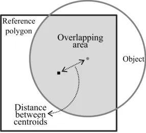
3.1 Geometric methods 176
Geometric methods rely on quantitative metrics that describe aspects of the geometric 177
correspondence between objects and polygons, often based on difference in area and position 178
(Winter, 2000). Figure 1 illustrates a typical case involving an object and polygon for which 179
the larger the overlapping area and/or the shorter the distance between their centroids, the 180
182
Figure 1. Geometric comparison between an object and polygon based on the overlapping 183
area (shaded area) and/or distance between centroids (dashed arrow). 184
3.1.1 Notation 185
Notation is necessary to assist the description of the metrics used by geometric methods. The 186
notation presented hereafter uses that defined in Clinton et al. (2010). Therefore, the notation 187
is transcribed below together with additional elements necessary to describe all the methods 188
covered. 189
The m objects constructed via image segmentation are denoted by yj (j=1, …, m), the n
190
polygons forming a reference data set by xi (i=1, …, n), and the l pixels of the segmented
191
remotely sensed data by zp(p=1, …,l). They define the following sets:
192
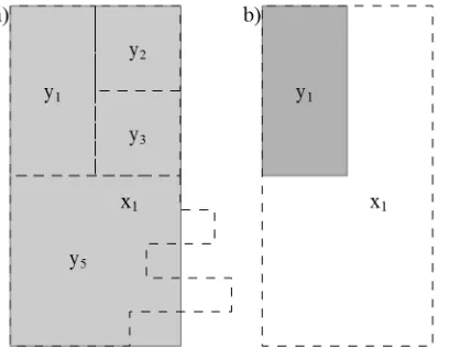
X={xi: i=1, …,n} is the set ofnpolygons (Figure 2a)
193
Y={yj: j=1, …,m} is the set ofmobjects of a segmentation output (Figure 2b)
194
S=X∩Y={sijk: area(xi∩yj)≠0} is the set of s intersection objects that result from the
195
spatial intersection (represented by symbol ∩) of X and Y; sijk is the kth object that
196
results from the spatial intersection of the ith polygon (xi) with the jth object (yj)
197
(Figure 2c) 198
Z={zp: p=1,…,l} is the set oflpixels of the segmented remotely sensed data.
199 200
Set S is the result of a spatial intersection of X and Y, which can be defined using common 201
geographical information systems. Note that the subscript k is needed to create a unique 202
symbol as the overlay of xi and yi can yield more than one discontinuous polygonal area (x1
203
and y6 in Figure 2). Set Z is simply the set of pixels that form the remotely sensed data
204
submitted to segmentation analysis, but its definition is nevertheless useful for describing 205
207
Figure 2. Sets X, Y, and S: (a) reference set X, (b) segmentation Y, and (c) intersection 208
S=X∩Y. In (c) yellow denotes one-to-one, blue denotes one-to-many, and pink denotes 209
many-to-many (Section 3.1.1.3). 210
The description of the methods also requires the use of symbols that characterize the sets X, 211
Y, S, and Z, and their members. For example, size() denotes the number of an item identified 212
in brackets, for example the number of objects that belong to Y – size(Y) – or the number of 213
pixels of an object – size(yj); and dist() is the distance between two items identified in
214
brackets, for example the centroids of yj and xi – dist(centroid(xi), centroid(yj)). This basic
215
notation is used to express more complex cases. For example, area(xi∩yj) is the area of the
216
geographical intersection of polygon xiand object yj. Other self-explanatory cases are used in
217
the notation adopted. Furthermore, mathematical symbols are also used, such as ¬ which is 218
the logical negation symbol and read as “not”, \ which is the complement symbol used in set 219
Subsets of X, Y, and S must be defined to assist the description of methods that follow four 221
different strategies: (i) Y is compared to X, (ii) X is compared to Y, (iii) S is compared to 222
both X and Y, and (iv) X and Y are compared to Z. In all of the cases, the definition of 223
subsets of X, Y, and S are used to decide which polygons xi, objects yj, and intersection
224
objects sijk corresponds to each other or to pixel zp, which is central to the calculation of
225
geometric metrics (presented in Section 3.1.2). 226
3.1.1.1 Set Y compared to set X
227
In image segmentation accuracy assessment most often the set Y is compared to set X. This 228
strategy typically involves the calculation of geometric metrics for the members of X, and 229
thus there is the need to identify which member(s) of Y correspond to each member of X. For 230
example, Figure 3a shows the set of objects that overlap and thus can be considered as 231
corresponding to a polygon xi. The specific objects that are actually considered as
232
corresponding depends on the method used, and the calculations related to each polygon xi
233
consider only the objects regarded as corresponding. Thus, it is useful to define the following 234
subsets of Y for each member of X: 235
Y~i is the subset of Y such that Y~i={yj: area(xi∩yj)≠0}
236
Yaiis a subset of Y~i such that Yai={yj: the centroid of xiis in yj}
237
Ybiis a subset of Y~i such that Ybi={yj: the centroid of yjis in xi}
238
Yciis a subset of Yi
~
such that Yci={yj: area(xi∩yj)/area(yj)>0.5}
239
Ydiis a subset of Yi
~
such that Ydi={yj: area(xi∩yj)/area(xi)>0.5}
240
Yeiis a subset of Yi
~
such that Yei={yj: area(xi∩yj)/area(yj)=1}
241
Yfiis a subset of Yi
~
such that Yfi={yj: area(xi∩yj)/area(yj)>0.55}
242
Ygiis a subset of Yi
~
such that Ygi={yj: area(xi∩yj)/area(yj)>0.75}
243
*
i
Y = Yai∪Ybi∪Yci∪Ydi
244
Yi is a subset of Yi
~
such that Yi={yj: max(area(xi∩yj))}.
245
The definition of subsets of Y expresses the variety of criteria of correspondence that has 246
been used. For example, some methods require the centroid of the objects to fall inside the 247
polygons, and Ybidenotes the set of objects whose centroid falls inside a specific polygon xi.
248
However, most of the criteria of correspondence used define a threshold of overlapping area 249
between polygons and objects. For example, at least half of the object’s area may have to 250
overlap a polygon for a positive correspondence to be considered; Yci denotes the set of
objects that comply with this criterion for a specific polygon xi. The selection of a specific
252
subset of Y depends on the method used. 253
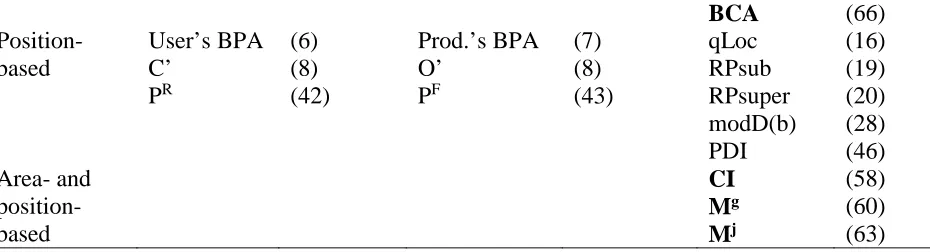
[image:12.595.200.404.133.291.2]254
Figure 3. Comparison between X and Y of Figure 2: (a) four potential objects (dashed lines) 255
corresponding to polygon x1 (grey background) when Y compares to X; (b) one potential
256
polygon (dashed line) corresponding to object y1(grey background) when X compares to Y.
257
3.1.1.2 Set X compared to set Y
258
When set X is compared to Y, geometric metrics are calculated for the members of Y, and 259
thus there is the need to identify which member(s) of X correspond to each member of Y. For 260
example, Figure 3b shows that one polygon overlap and thus can be considered as 261
corresponding to an object yj. The calculations related to each object yj consider only the
262
polygons regarded as corresponding, depending on the method used. Thus, it is useful to 263
define the following subsets of X for each member of Y: 264
X~ j is the subset of X such that
X
j~
={xi: area(yj∩xi)≠0}
265
Xcjis a subset of X~ j such that Xcj={xi: area(yj∩xi)/area(yj)>0.5}
266
Xj is a subset of X~ j such that X'j={xi: max(area(yj∩xi))}
267
Xj is a subset of X~ j such that Xj={xi: max(area(yj∩xi)/area(yj∪xi))}. 268
269
The subsets of X defined above represent the criteria of correspondence that have been used 270
when X is compared to Y. All the criteria define a threshold of overlapping area between 271
polygons and objects. For example, a polygon may have to overlap more than half of the 272
object’s area for a positive correspondence between objects and polygons; Xcidenotes the set
of polygons that comply with this criterion for a specific object yj. The selection of a specific
274
subset of X depends on the method used. 275
To describe two particular methods found in the literature (Costa et al., 2015; Liu and Xia, 276
2010), it is useful to define X not as the set ofnreference polygons, but the set oftthematic 277
classes represented in X. For example, if x3and x4in Figure 2 are two polygons representing
278
the same thematic class, ci, and both intersect the same object, y6, notation like area(ci∩y6)
279
can be used, where area(ci)=area(x3∪x4). Thus, similarly to above:
280
C={ci: i=1, …, t} is the set of tthematic classes represented in X; classes ci can also
281
be denoted as dias it is useful to describe a specific method (Costa et al., 2015).
282
When comparing C to Y, the following subset of C is identified for each yj:
283
C~ jis the subset of C such that C~ j={ci: area(ci∩yj)≠0}.
284
3.1.1.3 Set S compared to both sets X and Y
285
When set S is compared to both sets X and Y, three types of hierarchical relations between 286
polygons and objects emerge. The three types are one-to-one, one-to-many, and many-to-287
many relations (Figure 2). The first type occurs when xi and yj match perfectly. One-to-many
288
relations occur when xiintersects several objects orvice-versa. Many-to-many relations occur
289
when several discontinuous intersection objects correspond to a same xi and yj (e.g. sliver
290
intersection objects sijkalong the edges of xiand yj).
291
Given the three types of hierarchical object relations, the following subsets of S are defined: 292
S1={sijk: area(xi∩yj) = area(xi∪yj)} is the subset of all one-to-one objects
293
S2a={sijk: (one xi ∩ many yj) ˅ (many xi ∩ one yj)} is the subset of all one-to-many
294
relations 295
S2b={sijk: (one xi ∩ many yj) ˅ (many xi ∩ one yj); max(area(sijk)} is the subset of the
296
largest one-to-many relations 297
S3={sijk: one xi ∩ one yj over discontinuous areas; max(area(sijk)} is the subset of the
298
largest many-to-many relations. 299
Based on the above subsets, it is useful to define the subsets Sa=S1∪S2a ∪ S3, and Sb=S1 ∪
300
S2b∪ S3. Finally, subsets of Sa and Sb are defined for each xiand yj:
Saxi={sijk: area(sijk∩xi)≠0}
302
Sayj={sijk: area(sijk∩yj)≠0}
303
Sbxi={sijk: area(sijk∩xi)≠0}
304
Sbyj={sijk: area(sijk∩yj)≠0}
305
The definition of subsets Saxi, Sayj, Sbxi, and Sbyjare used in Möller et al. (2013) and Costa
306
et al. (2015). 307
3.1.1.4 Sets X and Y compared to set Z
308
To describe two particular methods found in the literature (Martin, 2003; Zhang et al., 2015a, 309
2015b), it is useful to consider the assessment framework at the pixel level and thus define 310
the following subsets of X and Y that correspond to each member of Z: 311
Xapis the subset of X such that Xap={xi: the centroid of zpis in xi}
312
Yapis the subset of Y such that Yap={yj: the centroid of zpis in yj}.
313
3.1.2 Available metrics 314
Geometric metrics are presented in Table 1 using the notation defined above, except four 315
cases that would require the definition of unnecessarily complex notation, and thus are 316
described as text (metrics 6, 7, 13 and 28). The metrics express the fundamental calculation 317
involving objects and polygons; each object, polygon, or intersection object receives a metric 318
value, which will tell something about the individual geometric accuracy of the objects 319
constructed. Assessing each areal entity individually is often referred to as local evaluation or 320
validation (Möller et al., 2013, 2007; Persello and Bruzzone, 2010). The subscripts i and j 321
used in the name of the metrics in Table 1 (e.g. Precisionij) indicate that the metrics are
322
calculated for the local level. These subscripts come from those used to identify the specific 323
polygon xiand object yjinvolved in the calculations.
324
Place table 1 near here.See Table 1 after the references.
325
Local metric values are commonly aggregated in a variety of ways to produce a single value 326
global evaluation or validation (Möller et al., 2013, 2007; Persello and Bruzzone, 2010). 328
Table 1 provides details on how the local metric values are aggregated for the global level in 329
the column headed Notes. Typically, the local values are summed or averaged in either one or 330
two steps, which in Clinton et al. (2010) is referred to as weighted and unweighted measures 331
respectively. In the first case, all the local values are aggregated in a straightforward fashion 332
(e.g. SimSize, metric 15). In the second case, the aggregation is undertaken first for each 333
individual polygon or object (depending of the strategy of comparison), and then for the 334
whole segmentation. For example, metric PIij(metric 22) is first aggregated for each polygon,
335
and then for the whole segmentation. Therefore, if for a given polygon, say x1, there are two
336
corresponding objects, y1and y2, then PI11and PI12are calculated according to metric 22.
337
Then, PI11and PI12are summed to calculate a single PI1value for polygon x1. This produces
338
nPIivalues (one for each polygon xi). Finally, thenPIivalues can be averaged to express
339
image segmentation accuracy as a whole, denoted as PI (without any subscript). 340
Showing the metrics for the local level facilitates comparison, but it was not possible to write 341
them all in the same style. For example, the LPiformula (metric 31) shows only the subscript
342
i (i.e. the subscript j is missing). This specific metric, calculated for polygons xi, needs
343
immediately to involve all the corresponding objects. In other cases, such as NSR (metric 344
39), the metric’s name in Table 1 shows no subscripts because the metric is calculated 345
directly as a global value for the whole segmentation output. 346
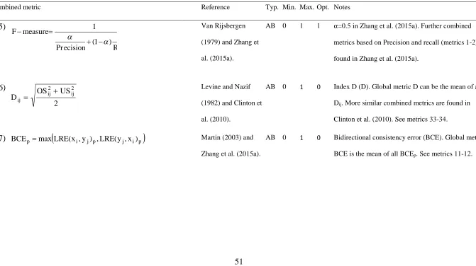
Oftentimes the purpose of calculating metrics, such as those of Table 1, is to combine them 347
later for the definition of further metrics. These are hereafter referred to as combined metrics 348
(Table 2). Several approaches have been proposed to combine geometric metrics, such as 349
metrics sum, and root mean square. The combination of metrics is done at either the local or 350
local level (OSijand USij) to produce a set of Dijvalues, which is then aggregated for the
352
global level. The F-measure (metric 55) combines two metrics at the global level (Precision 353
and Recall). A few more complex strategies have also been proposed for combining metrics, 354
namely clustering (CI, metric 58) and comparison of the cumulative distribution of the 355
metrics combined (Mgand Mj, metrics 60 and 63). 356
Place table 2 near here.See Table 2 after the references. 357
Further methods are found in the literature. Most of them are essentially the same as those 358
presented in Table 1 and Table 2. They are omitted here as are ambiguously described in the 359
original publications; for example, the correspondence between objects and polygons is 360
frequently unclear. Thus, they could not be translated to the notation defined in Section 3.1.1. 361
Methods not described here are, however, potentially useful and include those found in 362
Winter (2000); Oliveira et al. (2003); Radoux and Defourny (2007); Esch et al. (2008); 363
Corcoran et al. (2010); Korting et al. (2011); Verbeeck et al. (2012); Whiteside et al. (2014); 364
Michel et al. (2015) and Mikes et al. (2015). 365
3.1.3 Metrics use 366
Table 1 reveals that a variety of strategies has been adopted to compare objects and polygons. 367
Specifically, often the assessment is focused on the reference data set, and thus the 368
assessment proceeds by searching the objects that may correspond to each polygon (i.e. set Y 369
is compared to set X). For example, Recall (metric 2) uses this strategy. Sometimes the 370
assessment proceeds by searching the polygons that may correspond to each object (i.e. X is 371
compared to Y). Precision (metric 1) adopts this latter strategy. The remaining strategies 372
defined in Sections 3.1.1.3 and 3.1.1.4 are less frequently adopted, namely in three specific 373
Once the strategy of comparison between objects and polygons is specified, several criteria 375
may be used to determine the correspondence between objects and polygons. For example, 376
when set Y compares to set X a simple criterion is to consider only one corresponding object 377
for each of the polygons. This object may be the one that covers the largest extent of the 378
polygon (e.g. Recall, metric 2). However, a set of different criteria can be used. For example, 379
qLoc (metric 16) views an object as corresponding to a polygon if the centroid of the polygon 380
lies inside the object orvice versa. As a result, several objects may be identified as 381
corresponding to a single polygon. Only the corresponding objects and polygons are used for 382
calculating the geometric metrics. 383
Most of the metrics presented in Table 1 and Table 2 are based on proportions of overlapping 384
area. For example, Precision (metric 1) is based on the calculation of the proportion of the 385
area that each object has in common with the corresponding polygon. On the other hand, 386
some metrics are based on the distance between centroids. For example, qLoc (metric 16) is 387
based on the distance between the centroid of each of the polygons to that of the 388
corresponding objects. Metrics that focus on area are often referred to as area coincidence-389
based or area-based metrics. The metrics that focus on position are often referred to as 390
boundary coincidence-based, location-based, or position-based metrics (Cheng et al., 2014; 391
Clinton et al., 2010; Montaghi et al., 2013; Whiteside et al., 2014; Winter, 2000). 392
A substantial proportion of the metrics detect either under-segmentation or over-segmentation 393
error. This may be unexpected as commonly a balanced result is desired, but it informs on 394
what type of error dominates. This may be used, for example, to parameterize a segmentation 395
algorithm. For this reason, normally metrics that detect and measure under- or over-396
segmentation error are calculated separately, but combined later (Table 2) to provide a 397
position-based metrics are sometimes combined to provide a comprehensive assessment of 399
image segmentation accuracy from a geometric point of view (Möller et al., 2013). The 400
combined metrics are typically the outcome of an image segmentation accuracy assessment 401
based on a geometric approach. The possible values of these metrics are in the range between 402
0 and 1, and they may be used to rank a set of image segmentation outputs based on their 403
expected suitability for image classification. To assist in the comparison of all metrics 404
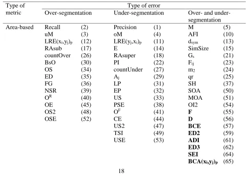
presented here, the metrics of Table 1 and Table 2 are grouped in Table 3 by type of error 405
measured (over- and/or under-segmentation) and geometric feature considered (area and/or 406
[image:18.595.61.545.424.772.2]position). 407
Table 3. Geometric metrics of tables 1 and 2 grouped by type of error measured (over-408
segmentation and/or under-segmentation) and type of metric (area-based and/or position-409
based). Combined metrics of table 2 are in bold. 410
Type of metric
Type of error
Over-segmentation Under-segmentation Over- and under-segmentation Area-based Recall
uM
LRE(xi,yj)p
RAsub countOver BsO OS ED FG NSR OR OE OS2 OSE (2) (3) (12) (17) (26) (30) (34) (35) (36) (39) (40) (45) (48) (52) Precision oM
LRE(yj,xi)p
E RAsuper PI countUnder Aj LP EP US PSE OF CE US2 TSI USE (1) (4) (11) (14) (18) (22) (27) (29) (31) (32) (33) (38) (41) (44) (47) (49) (53) M AFI dsym SimSize Gs Fij m2 qr SH SOA MOA OI2 F D BCE ED2 ADI ED3 SEI
BCA(xi,yj)p
BCA (66)
Position-based
User’s BPA C’
PR
(6) (8) (42)
Prod.’s BPA O’
PF
(7) (8) (43)
qLoc RPsub RPsuper modD(b) PDI
(16) (19) (20) (28) (46) Area- and
position-based
CI
Mg
Mj
(58) (60) (63) 411
3.2 Non-geometric methods 412
A small number of non-geometric methods have been proposed (Table 4). Typically, this 413
category of methods does not require an overlay operation between a polygonal reference 414
data set and the image segmentation output under evaluation as they need not to be spatially 415
coincident. Polygons may not even be used. The requirement common to all non-geometric 416
methods is that the land cover class(es) associated with the objects are known. Note that non-417
geometric methods are not able to explicitly inform on which type of error, under- or over-418
[image:19.595.74.539.73.199.2]segmentation, predominates. 419
Table 4. Non-geometric methods for supervised assessment of image segmentation accuracy. 420
All metrics detect under- and over-segmentation error. 421
Reference Focus of the method Polygons neededa
Wang et al. (2004) Objects’ content (spectral separability of classes using the
Bhattacharyya distance).
No
Laliberte and
Rango (2009)
Classifier (Decision trees classification accuracy and Gini index). No
Anders et al. (2011) Objects’ content (difference among objects and polygons on the
frequency distribution of characterizing topographic attributes).
Yes
Yang et al. (2017) Classifier (classification uncertainty) No
aThe reference data set used is required in the form of polygons
Non-geometric methods essentially follow two approaches to assess the accuracy of image 423
segmentation. The first approach focuses on the content of the objects. Anders et al. (2011) 424
compared the content of objects and polygons using the frequency distribution of their 425
topographic attributes such as slope angle while mapping geomorphological features. Smaller 426
differences between frequency distributions calculated from objects and polygons of the same 427
geomorphological feature type indicated greater segmentation accuracy. However, most of 428
the non-geometric methods dispense with polygons and only require objects with known 429
spectral and thematic content. These objects may be represented in the spectral space used in 430
the segmentation analysis where the objects of different land cover classes are desirable to lie 431
in different regions so that later a classifier can allocate them to the correct class. The 432
separability of the objects in the spectral space as a function of the land cover classes they 433
represent is regarded as indicative of segmentation accuracy, and this can be assessed based 434
on, for example, the Bhattacharyya distance (Fukunaga, 1990). This is possibly the most used 435
non-geometric method (Li et al., 2015; Radoux and Defourny, 2008; Wang et al., 2004; Xun 436
and Wang, 2015). 437
The second approach used in non-geometric methods assesses image segmentation using a 438
classifier. Specifically, a series of preliminary classifications are undertaken with a set of 439
image segmentation outputs, and the classifier is used to rank the segmentations based on 440
their suitability for image classification. For example, a sample of the objects of the image 441
segmentation under evaluation can be used to train a decision tree, and the impurity of the 442
terminal nodes can be regarded as indicative of classification success; large accuracy of 443
image segmentation is expected to be related to low node impurity (Laliberte and Rango, 444
2009). Most often, however, traditional estimators of classification accuracy such as overall 445
which of a set of segmentation outputs affords the largest classification accuracy. In this case, 447
samples of the objects constructed can be used for training and testing a classifier by means 448
of out-of-bag estimate or cross-validation (Laliberte and Rango, 2009; Smith, 2010). 449
Classification uncertainty rather than accuracy can also be used. If a fuzzy classifier is 450
employed, the way in which the probability of class membership is partitioned between the 451
classes can be used to calculate classification uncertainty, for example based on entropy 452
measures. Segmentation accuracy may be viewed as negatively related to the magnitude of 453
classification uncertainty (Yang et al., 2017). 454
The second approach of non-geometric image segmentation accuracy assessment, especially 455
when classification accuracy expressed by traditional estimators such as overall accuracy is 456
considered, may appear similar to traditional classification accuracy assessment, but they are 457
different things. The former uses the training sample to assess the accuracy of the preliminary 458
classifications while the latter assesses the quality of the final mapping product and requires 459
an independent testing sample. Sometimes traditional classification accuracy assessment is 460
nevertheless used to assess indirectly image segmentation accuracy (e.g. Kim et al., 2009; Li 461
et al., 2011). When used, the focus is typically on a comparison among the accuracy values of 462
a set of final classifications (Foody, 2009, 2004), with each produced with different image 463
segmentation outputs. The differences are caused not only by the image segmentations used, 464
but the entire approach to image classification. This may be well suited for applications 465
focused on the final mapping products, but implies possibly impractical labour and resources 466
4
Selecting a method
468The selection of a method to assess the accuracy of image segmentation is a complex 469
decision, and here it is suggested to tackle that decision from two central perspectives: the 470
application in-hand, and the pros and cons of the methods. These issues should be considered 471
holistically although discussed separately hereafter. 472
4.1 Application in-hand 473
The purpose of the application in-hand should be considered, and there are two main 474
situations. First, the applications are focused on just a fraction of the classes in which a 475
landscape may be categorized. These applications use image segmentation primarily for 476
object recognition and extraction, such as buildings and trees in urban environments (e.g. 477
Belgiu and Drǎguţ, 2014; Sebari and He, 2013). The desired characteristics of the objects are 478
likely to be geometric, such as position and shape. Several methods may be appropriate, such 479
as shape error (metric 37); the segmentation output indicated as optimal will in principle be 480
formed by objects that most resemble the desired shapes represented in the reference data set. 481
Alternatively, the relative overlapping areas between objects and polygons may be 482
maximised. This strategy may benefit from area-based metrics designed for object 483
recognition, such as SEI (metric 64). 484
The second main situation corresponds to wall-to-wall land cover classification and mapping 485
(e.g Bisquert et al. 2015; Strasser and Lang 2015). In this case, the geometric properties of 486
the objects may be considered important as in the first situation described above, and hence 487
geometric methods may be used. However, the thematic information associated with the 488
objects is commonly regarded as more important than the geometrical representation. In this 489
represented in the final map is preferred. Geometric methods can still be used, and area-based 491
methods may be appropriate, which will in principle suggest as optimal the segmentation 492
output formed by objects that represent the largest amount of area of the corresponding 493
polygons. This gives the classification stage the opportunity of maximising the area correctly 494
classified and thus the overall accuracy of the map. Non-geometric methods can also be used 495
(Table 4). There is less experience in the use of this category of methods, but it is potentially 496
useful when the geometry of the objects does not have to meet predefined requirements. 497
An intermediate situation is also possible in that both the geometric and thematic properties 498
of the objects are regarded as important. In this case, methods that combine different 499
approaches for the accuracy assessment may be used, for example focused on the relative 500
position and area of overlap between objects and polygons (Möller et al., 2013, 2007). 501
However, there is no need to select just one method, and assembling multiple methods is a 502
valid option (Clinton et al., 2010). Different methods, including geometric and non-geometric 503
methods, can be used together to address all the specific properties of the objects considered 504
as relevant as long as the set of methods used fits the purpose of the application in-hand. 505
Another relevant aspect of the application in-hand is the relative importance of under- and 506
over-segmentation error. Image segmentation is typically conducted to trade-off and 507
minimize under- and over-segmentation error, but over-segmentation may be needed to 508
address conveniently the problem under analysis. Specifically, small objects, sometimes 509
called primitive objects (Dronova, 2015), may be needed for modelling complex classes that 510
are not directly related to spectral data, such as habitats (Strasser and Lang, 2015). The final 511
land cover classes can be delineated later, for example, based on knowledge-driven semantic 512
rules (Gu et al., 2017). If no primitive objects are needed, and the border of the final land 513
nevertheless to recognize that under- and over-segmentation error are not always equally 515
serious, especially if the application is interested more on the thematic rather than the 516
geometric properties of the objects. Multiple authors have expressed their preference for 517
over- rather than under-segmentation error as the latter is associated with relatively small 518
classification accuracy (Gao et al., 2011; Hirata and Takahashi, 2011; Lobo, 1997; Wang et 519
al., 2004). Under-segmentation error produces objects that correspond to more than one class 520
on the ground and thus may represent an important origin of misclassification or land cover 521
map error. Therefore, using methods able to inform on the level of over- and under-522
segmentation error may be convenient, such as that proposed by Möller et al. (2013). 523
The third and last aspect highlighted here relates to the potential importance of thematic 524
errors associated with under-segmentation error. That is, the impact of under-segmentation 525
error may depend on the classes associated with under-segmented objects. This is because the 526
needs of the individual users may vary greatly in their sensitivity to misclassifications as a 527
function of the classes involved (Bontemps et al., 2012; Comber et al., 2012). Traditionally, 528
supervised methods consider all segmentation errors as equally serious, but under-529
segmentation errors can in fact be weighted as a function of the classes involved. This is the 530
situation with the geometric method proposed by Costa et al. (2015) (metric 63) and non-531
geometric methods that use a classifier to perform a preliminary series of classifications, 532
whose results can be expressed through weighted estimators of classification accuracy, such 533
as the Stehman's (1999) map value V. 534
4.2 Methods’ pros and cons 535
A consideration of the potential implications associated with the approach of the assessment 536
be very practical, but are unable to explicitly inform on which type of segmentation error 538
predominates. That information may be useful for guiding the definition of segmentation 539
settings. If this limitation is undesirable, a geometric method suited to detecting segmentation 540
error explicitly should be preferred. However, the need of defining criteria of correspondence 541
between objects and polygons should be considered carefully as it impacts on the accuracy 542
assessment. The geometric methods proposed by Yang et al. (2015) (SEI, metric 64), Su and 543
Zhang (2017) (OSE, metric 52), and Möller et al. (2013) (Mg, metric 60) pay particular
544
attention to this issue. 545
Quantitative comparisons of different methods should be undertaken. Several comparative 546
studies dedicated to geometric methods have been published (Clinton et al., 2010; Räsänen et 547
al., 2013; Whiteside et al., 2014; Yang et al., 2015), and some of them (e.g. Clinton et al., 548
2010; Verbeeck et al., 2012) observed that different methods can indicate very different 549
segmentation outputs as optimal. Thus, special attention should be given to potential bias of 550
the methods. For example, Radoux and Defourny (2008) found that spectral separability 551
measures used in non-geometric methods may be insensitive to under-segmentation error, and 552
thus indicate a segmentation as optimal while notably under-segmented; Witharana and 553
Civco (2014) found that the sensitivity of Euclidean distance 2 (ED2, metric 59) to the 554
accuracy of the objects depends of the scale of the analysis. 555
Finally, it should be noted that estimated bias in image segmentation accuracy assessment is 556
not caused merely by unsuitable choice of methods or their potential flaws, but the protocol 557
used for their implementation. Typically, some reference data are available for a sample of 558
the entire area to be mapped, and thus limited data are used to infer an accuracy estimate to 559
represent the entire area. Therefore, the nature of sampling is an issue that will impact on the 560
using a probability sampling design, which must incorporate a randomization component that 562
has a non-zero probability of selection for each object into the sample. Consideration of 563
general sampling and statistical principles for defining samples is recommended (Olofsson et 564
al., 2014; Stehman and Czaplewski, 1998). 565
5
Discussion
5665.1 Current status 567
Image segmentation accuracy assessment appears to be in a relatively early stage of 568
maturation in land cover mapping applications. Often no information on the assessment 569
produced is given, and qualitative assessment based on visual interpretation is widely used. 570
This situation may be a result of several factors. For example, the lack of a solid background 571
in image segmentation accuracy assessment and reliable recommendations for method 572
selection may be a motivation for neglecting a quantitative accuracy assessment. Another 573
factor may be related to the difficulty of implementing most of the methods proposed in the 574
literature. Many analysts of remote sensing data depend on standard software and have no 575
resources or expertise to implement new methods. This may also be a reason why comparison 576
among methods has been addressed in a relatively small number of studies. There are some 577
initiatives to implement supervised methods and make them available to the public (Mikes et 578
al. 2015), but further work should be done in this respect. Clinton et al. (2010), Montaghi et 579
al. (2013), Eisank et al. (2014), and Novelli et al. (2017) provide additional information on 580
how to access software that includes supervised methods for image segmentation accuracy 581
assessment. 582
Supervised methods were reviewed here and grouped into two categories: geometric and non-583
of them are similar. This is the case of area(xi∩yj)/area(yj), which appears in metrics 1, 18,
585
33, and 47. Winter (2000) demonstrated that only seven metrics are possible to derive from 586
an area-based approach if they are free of dimension, normalized, and symmetric (i.e. there is 587
a single and mutual correspondence between objects and polygons). However, several 588
correspondence criteria and strategies of comparison between objects and polygons can be 589
specified, and thus the number of area-based metrics can proliferate. This is essentially the 590
case of metrics 1, 18, 33 and 47, which are calculated with different criteria of 591
correspondence between objects and polygons (Xj, Y~i , Yi, and Yci∪Ydi, respectively).
592
The ways the local metric values are used to produce a global accuracy value also vary. 593
These apparently slight differences may, however, impact substantially on the assessment as 594
different calculations are involved. 595
Selecting an appropriate method for image segmentation accuracy assessment is not obvious. 596
The pros and cons of the potential methods, such as ease of use and bias, should be taken into 597
account. However, it is noted that there is often neither a right nor wrong method. The 598
suitability of a method will ultimately depend on how it fits with the application in-hand. 599
5.2 Research needs 600
Quantitative studies similar to Clinton et al. (2010) and Witharana and Civco (2014) should 601
be done to exhaustively test and compare the supervised methods used in the remote sensing 602
community. Non-geometric methods should be inspected as they have been neglected in 603
quantitative studies. Moreover, the studies should be conducted under different contexts that 604
may represent different types of applications, such as object recognition, and wall-to-wall 605
classification accuracies is required, as often relations were not simple (Belgiu and Drǎguţ, 607
2014; Costa et al., 2017; Räsänen et al., 2013; Verbeeck et al., 2012). 608
Finally, the concept of over- and under-segmentation error should be revisited. Commonly, as 609
in this paper, segmentation error is defined relative to the reference data used, and thus the 610
concept lacks theoretical robustness. For example using reference data representing final land 611
cover classes to be mapped or primitive objects impacts on the results. Primitive objects have 612
a more spectral rather than thematic significance, and this may influence the assessment, 613
including the selection of the assessment approach, supervised or unsupervised. However, 614
theory and concepts related to object-based image analysis are generally incipient (Blaschke 615
et al., 2014; Ma et al., 2017), and comparing supervised and unsupervised methods which 616
often focus on thematic and primitive objects, respectively, has not received much attention. 617
6
Conclusions
618Accuracy assessment is an important component of an image segmentation analysis, but is 619
not mature. It has been much undertaken through visual inspection possibly for practical 620
reasons while many quantitative approaches and methods have been proposed. Most often 621
these methods are supervised and focus on the geometry of the objects constructed and 622
polygons taken as reference data. However, other approaches may be used. The spectrum of 623
methods available is large, and it is difficult to select consciously suitable methods for 624
particular applications. There are at least three important questions that should be asked 625
during the selection of supervised methods for image segmentation accuracy assessment: (i) 626
the goal of the application; (ii) the relative importance of under- and over-segmentation error 627
(including a possible varying sensitivity to thematic issues associated to under-segmentation); 628
methods, but further research is needed to improve the standards of image segmentation 630
accuracy assessment, otherwise there is the risk of using methods unsuitable or sub-optimal 631
for the application in-hand. 632
Acknowledgements
633Hugo Costa was supported by the PhD Studentship SFRH/BD/77031/2011 from the 634
“Fundação para a Ciência e Tecnologia” (FCT), funded by the “Programa Operacional 635
Potencial Humano” (POPH) and the European Social Fund. The paper benefited from 636
valuable comments received from the editors and anonymous reviewers. 637
References
638Abeyta, A., Franklin, J., 1998. The accuracy of vegetation stand boundaries derived from 639
image segmentation in a desert environment. Photogramm. Eng. Remote Sensing 64, 640
59–66. 641
Anders, N.S., Seijmonsbergen, A.C., Bouten, W., 2011. Segmentation optimization and 642
stratified object-based analysis for semi-automated geomorphological mapping. Remote 643
Sens. Environ. 115, 2976–2985. doi:10.1016/j.rse.2011.05.007 644
Basaeed, E., Bhaskar, H., Hill, P., Al-Mualla, M., Bull, D., 2016. A supervised hierarchical 645
segmentation of remote-sensing images using a committee of multi-scale convolutional 646
neural networks. Int. J. Remote Sens. 37, 1671–1691. 647
doi:10.1080/01431161.2016.1159745 648
Beauchemin, M., Thomson, K.P.B., Edwards, G., 1998. On the Hausdorff distance used for 649
the evaluation of segmentation results. Can. J. Remote Sens. 24, 3–8. 650
doi:10.1080/07038992.1998.10874685 651
Belgiu, M., Drǎguţ, L., 2014. Comparing supervised and unsupervised multiresolution 652
segmentation approaches for extracting buildings from very high resolution imagery. 653
ISPRS J. Photogramm. Remote Sens. 96, 67–75. doi:10.1016/j.isprsjprs.2014.07.002 654
Bisquert, M., Bégué, A., Deshayes, M., 2015. Object-based delineation of homogeneous 655
landscape units at regional scale based on MODIS time series. Int. J. Appl. Earth Obs. 656
Geoinf. 37, 72–82. doi:10.1016/j.jag.2014.10.004 657
Blaschke, T., 2010. Object based image analysis for remote sensing. ISPRS J. Photogramm. 658
Blaschke, T., Hay, G.J., Kelly, M., Lang, S., Hofmann, P., Addink, E.A., Queiroz Feitosa, R., 660
van der Meer, F., van der Werff, H., van Coillie, F., Tiede, D., 2014. Geographic Object-661
Based Image Analysis – Towards a new paradigm. ISPRS J. Photogramm. Remote Sens. 662
87, 180–191. doi:10.1016/j.isprsjprs.2013.09.014 663
Bontemps, S., Herold, M., Kooistra, L., van Groenestijn, A., Hartley, A., Arino, O., Moreau, 664
I., Defourny, P., 2012. Revisiting land cover observation to address the needs of the 665
climate modeling community. Biogeosciences 9, 2145–2157. doi:10.5194/bg-9-2145-666
2012 667
Bradley, B.A., 2014. Remote detection of invasive plants: A review of spectral, textural and 668
phenological approaches. Biol. Invasions 16, 1411–1425. doi:10.1007/s10530-013-669
0578-9 670
Cardoso, J.S., Corte-Real, L., 2005. Toward a generic evaluation of image segmentation. 671
IEEE Trans. Image Process. 14, 1773–1782. doi:10.1109/TIP.2005.854491 672
Carleer, A.P., Debeir, O., Wolff, E., 2005. Assessment of very high spatial resolution satellite 673
image segmentations. Photogramm. Eng. Remote Sensing 71, 1285–1294. 674
doi:10.14358/PERS.71.11.1285 675
Cheng, J., Bo, Y., Zhu, Y., Ji, X., 2014. A novel method for assessing the segmentation 676
quality of high-spatial resolution remote-sensing images. Int. J. Remote Sens. 35, 3816– 677
3839. doi:10.1080/01431161.2014.919678 678
Clinton, N., Holt, A., Scarborough, J., Yan, L., Gong, P., 2010. Accuracy assessment 679
measures for object-based image segmentation goodness. Photogramm. Eng. Remote 680
Sensing 76, 289–299. 681
Coillie, F.M.B. Van, Gardin, S., Anseel, F., 2014. Variability of operator performance in 682
remote-sensing image interpretation: the importance of human and external factors. Int. 683
J. Remote Sens. 35, 754–778. doi:10.1080/01431161.2013.873152 684
Comber, A., Fisher, P., Brunsdon, C., Khmag, A., 2012. Spatial analysis of remote sensing 685
image classification accuracy. Remote Sens. Environ. 127, 237–246. 686
doi:10.1016/j.rse.2012.09.005 687
Corcoran, P., Winstanley, A., Mooney, P., 2010. Segmentation performance evaluation for 688
object-based remotely sensed image analysis. Int. J. Remote Sens. 31, 617–645. 689
doi:10.1080/01431160902894475 690
Costa, G.A.O.P., Feitosa, R.Q., Cazes, T.B., Feijó, B., 2008. Genetic adaptation of 691
segmentation parameters, in: Blaschke, T., Lang, S., Hay, G.J. (Eds.), Object-Based 692
Image Analysis. Springer Berlin Heidelberg, Berlin, Heidelberg, pp. 679–695. 693
doi:10.1007/978-3-540-77058-9_37 694
Costa, H., Foody, G.M., Boyd, D.S., 2015. Integrating user needs on misclassification error 695
sensitivity into image segmentation quality assessment. Photogramm. Eng. Remote 696
Costa, H., Foody, G.M., Boyd, D.S., 2017. Using mixed objects in the training of object-698
based image classifications. Remote Sens. Environ. 190, 188–197. 699
doi:10.1016/j.rse.2016.12.017 700
Crevier, D., 2008. Image segmentation algorithm development using ground truth image data 701
sets. Comput. Vis. Image Underst. 112, 143–159. doi:10.1016/j.cviu.2008.02.002 702
Drăguţ, L., Csillik, O., Eisank, C., Tiede, D., 2014. Automated parameterisation for multi-703
scale image segmentation on multiple layers. ISPRS J. Photogramm. Remote Sens. 88, 704
119–127. doi:10.1016/j.isprsjprs.2013.11.018 705
Drǎguţ, L., Tiede, D., Levick, S.R., 2010. ESP: a tool to estimate scale parameter for 706
multiresolution image segmentation of remotely sensed data. Int. J. Geogr. Inf. Sci. 24, 707
859–871. doi:10.1080/13658810903174803 708
Dronova, I., 2015. Object-based image analysis in wetland research: A review. Remote Sens. 709
7, 6380–6413. doi:10.3390/rs70506380 710
Eisank, C., Smith, M., Hillier, J., 2014. Assessment of multiresolution segmentation for 711
delimiting drumlins in digital elevation models. Geomorphology 214, 452–464. 712
doi:10.1016/j.geomorph.2014.02.028 713
Esch, T., Thiel, M., Bock, M., Roth, A., Dech, S., 2008. Improvement of image segmentation 714
accuracy based on multiscale optimization procedure. IEEE Geosci. Remote Sens. Lett. 715
5, 463–467. doi:10.1109/LGRS.2008.919622 716
Feitosa, R.Q., Ferreira, R.S., Almeida, C.M., Camargo, F.F., Costa, G.A.O.P., 2010. 717
Similarity metrics for genetic adaptation of segmentation parameters, in: 3rd 718
International Conference on Geographic Object-Based Image Analysis (GEOBIA 2010). 719
The International Archives of the Photogrammetry, Remote Sensing and Spatial 720
Information Sciences, Ghent. 721
Feizizadeh, B., Blaschke, T., Tiede, D., Moghaddam, M.H.R., 2017. Evaluating fuzzy 722
operators of an object-based image analysis for detecting landslides and their changes. 723
Geomorphology 293, Part A, 240–254. 724
doi:https://doi.org/10.1016/j.geomorph.2017.06.002 725
Foody, G.M., 2009. Classification accuracy comparison: Hypothesis tests and the use of 726
confidence intervals in evaluations of difference, equivalence and non-inferiority. 727
Remote Sens. Environ. 113, 1658–1663. doi:10.1016/j.rse.2009.03.014 728
Foody, G.M., 2004. Thematic map comparison: Evaluating the statistical significance of 729
differences in classification accuracy. Photogramm. Eng. Remote Sensing 70, 627–633. 730
doi:10.14358/PERS.70.5.627 731
Fukunaga, M., 1990. Introduction to statistical pattern recognition, 2nd ed. Academic Press, 732
San Diego. 733
Gao, Y., Mas, J.F., Kerle, N., Pacheco, J.A.N., 2011. Optimal region growing segmentation 734
doi:10.1080/01431161003777189 736
Gu, H., Li, H., Yan, L., Liu, Z., Blaschke, T., Soergel, U., 2017. An Object-Based Semantic 737
Classification Method for High Resolution Remote Sensing Imagery Using Ontology. 738
Remote Sens. . doi:10.3390/rs9040329 739
Hirata, Y., Takahashi, T., 2011. Image segmentation and classification of Landsat Thematic 740
Mapper data using a sampling approach for forest cover assessment. Can. J. For. Res. 741
41, 35–43. doi:10.1139/X10-130 742
Hultquist, C., Chen, G., Zhao, K., 2014. A comparison of Gaussian process regression, 743
random forests and support vector regression for burn severity assessment in diseased 744
forests. Remote Sens. Lett. 5, 723–732. doi:10.1080/2150704X.2014.963733 745
Janssen, L.L.F., Molenaar, M., 1995. Terrain objects, their dynamics and their monitoring by 746
the integration of GIS and remote sensing. IEEE Trans. Geosci. Remote Sens. 33, 749– 747
758. doi:10.1109/36.387590 748
Kim, M., Madden, M., Warner, T.A., 2009. Forest type mapping using object-specific texture 749
measures from multispectral Ikonos Imagery: Segmentation quality and image 750
classification issues. Photogramm. Eng. Remote Sensing 75, 819–829. 751
Korting, T.S., Dutra, L.V., Fonseca, L.M.G., 2011. A resegmentation approach for detecting 752
rectangular objects in high-resolution imagery. IEEE Geosci. Remote Sens. Lett. 8, 621– 753
625. doi:10.1109/LGRS.2010.2098389 754
Laliberte, A.S., Rango, A., 2009. Texture and scale in object-based analysis of subdecimeter 755
resolution unmanned aerial vehicle (UAV) imagery. IEEE Trans. Geosci. Remote Sens. 756
47, 1–10. doi:10.1109/TGRS.2008.2009355 757
Lang, S., Albrecht, F., Kienberger, S., Tiede, D., 2010. Object validity for operational tasks 758
in a policy context. J. Spat. Sci. 55, 9–22. doi:10.1080/14498596.2010.487639 759
Lang, S., Kienberger, S., Tiede, D., Hagenlocher, M., Pernkopf, L., 2014. Geons – domain-760
specific regionalization of space. Cartogr. Geogr. Inf. Sci. 41, 214–226. 761
doi:10.1080/15230406.2014.902755 762
Levine, M.D., Nazif, A.M., 1982. An experimental rule based system for testing low level 763
segmentation strategies, in: Preston, K., Uhr, L. (Eds.), Multicomputers and Image 764
Processing: Algorithms and Programs. Academic Press, New York, pp. 149–160. 765
Li, D., Ke, Y., Gong, H., Li, X., 2015. Object-based urban tree species classification using bi-766
temporal WorldView-2 and WorldView-3 images. Remote Sens. 7, 16917–16937. 767
doi:10.3390/rs71215861 768
Li, P., Guo, J., Song, B., Xiao, X., 2011. A multilevel hierarchical image segmentation 769
method for urban impervious surface mapping using very high resolution imagery. IEEE 770
J. Sel. Top. Appl. Earth Obs. Remote Sens. 4, 103–116. 771
Liu, D., Xia, F., 2010. Assessing object-based classification: Advantages and limitations. 773
Remote Sens. Lett. 1, 187–194. doi:10.1080/01431161003743173 774
Liu, J., Li, P., Wang, X., 2015. A new segmentation method for very high resolution imagery 775
using spectral and morphological information. ISPRS J. Photogramm. Remote Sens. 776
101, 145–162. doi:10.1016/j.isprsjprs.2014.11.009 777
Liu, Y., Bian, L., Meng, Y., Wang, H., Zhang, S., Yang, Y., Shao, X., Wang, B., 2012. 778
Discrepancy measures for selecting optimal combination of parameter values in object-779
based image analysis. ISPRS J. Photogramm. Remote Sens. 68, 144–156. 780
doi:10.1016/j.isprsjprs.2012.01.007 781
Lobo, A., 1997. Image segmentation and discriminant analysis for the identification of land 782
cover units in ecology. IEEE Trans. Geosci. Remote Sens. 35, 1136–1145. 783
doi:10.1109/36.628781 784
Lucieer, A., Stein, A., 2002. Existential uncertainty of spatial objects segmented from 785
satellite sensor imagery. Geosci. Remote Sensing, IEEE Trans. 40, 2518–2521. 786
doi:10.1109/TGRS.2002.805072 787
Ma, L., Li, M., Ma, X., Cheng, L., Du, P., Liu, Y., 2017. A review of supervised object-based 788
land-cover image classification. ISPRS J. Photogramm. Remote Sens. 130, 277–293. 789
doi:10.1016/j.isprsjprs.2017.06.001 790
Marpu, P.R., Neubert, M., Herold, H., Niemeyer, I., 2010. Enhanced evaluation of image 791
segmentation results. J. Spat. Sci. 55, 55–68. doi:10.1080/14498596.2010.487850 792
Martin, D.R., 2003. An empirical approach to grouping and segmentation. ECS Department, 793
University of California. 794
Matikainen, L., Karila, K., Hyyppä, J., Litkey, P., Puttonen, E., & Ahokas, E. (2017). Object-795
based analysis of multispectral airborne laser scanner data for land cover classification 796
and map updating.ISPRS Journal of Photogrammetry and Remote Sensing,128, 298– 797
313. http://doi.org/https://doi.org/10.1016/j.isprsjprs.2017.04.005 798
Michel, J., Youssefi, D., Grizonnet, M., 2015. Stable mean-shift algorithm and its application 799
to the segmentation of arbitrarily large remote sensing images. IEEE Trans. Geosci. 800
Remote Sens. 53, 952–964. doi:10.1109/TGRS.2014.2330857 801
Mikes, S., Haindl, M., Scarpa, G., Gaetano, R., 2015. Benchmarking of remote sensing 802
segmentation methods. IEEE J. Sel. Top. Appl. Earth Obs. Remote Sens. 8, 2240–2248. 803
doi:10.1109/JSTARS.2015.2416656 804
Möller, M., Birger, J., Gidudu, A., Gläßer, C., 2013. A framework for the geometric accuracy 805
assessment of classified objects. Int. J. Remote Sens. 34, 8685–8698. 806
doi:10.1080/01431161.2013.845319 807
Möller, M., Lymburner, L., Volk, M., 2007. The comparison index: A tool for assessing the 808
accuracy of image segmentation. Int. J. Appl. Earth Obs. Geoinf. 9, 311–321. 809