Orthogonal forward selection for constructing the radial basis function network with tunable nodes

the Radial Basis Function Network with Tunable Nodes

Sheng Chen1, Xia Hong2, and Chris J. Harris1

1 _{School of Electronics and Computer Science,}

University of Southampton, Southampton SO17 1BJ, UK

{sqc, cjh}@ecs.soton.ac.uk

2 _{Department of Cybernetics, University of Reading,}

Reading RG6 6AY, UK [email protected]

Abstract. An orthogonal forward selection (OFS) algorithm based on the leave-one-out (LOO) criterion is proposed for the construction of radial basis function (RBF) networks with tunable nodes. This OFS-LOO algorithm is computation-ally efficient and is capable of identifying parsimonious RBF networks that gen-eralise well. Moreover, the proposed algorithm is fully automatic and the user does not need to specify a termination criterion for the construction process.

1

Introduction

The radial basis function (RBF) network is a popular artificial neural network structure that has found wide applications in machine learning and engineering. The parameters of the RBF network include its centre vectors and variances of the basis functions as well as the weights that connect the RBF nodes to its output node. The parameters of a RBF network can be learned via nonlinear optimisation using the gradient based algorithm [1], the evolutionary algorithm [2] or the E-M algorithm [3]. Such a nonlinear learning approach is computationally expensive and may encounter the local minima problem. Additionally, the network structure or the number of RBF nodes has to be determined via other means. Alternatively, clustering algorithms can be applied to find the RBF centre vectors as well as the associated basis function variances [4]-[6]. This leaves the RBF weights to be determined by the usual linear least squares solution. Again, the number of the clusters has to be determined via other means, such as cross validation.

A popular approach for constructing RBF networks is to formulate the problem as a linear learning one by considering the training input data points as candidate RBF centres and employing a common variance for every RBF node. A parsimonious RBF network is then identified using the efficient orthogonal least squares (OLS) algorithm [7]-[10]. Similarly, the support vector machine (SVM) and other sparse kernel mod-elling methods [11]-[17] also fit the kernel centres to the training input data points and adopt a common variance for every kernels. A sparse kernel representation is then sought. Since the common variance is not provided by the learning algorithm, it has to be determined via cross validation. In a recent work [10], a locally regularised OLS

D.S. Huang, X.-P. Zhang, G.-B. Huang (Eds.): ICIC 2005, Part I, LNCS 3644, pp. 777–786, 2005. c

(LROLS) algorithm based on the leave-one-out (LOO) mean square error criterion has been proposed, which compares favourably with other existing state-of-the-art sparse kernel modelling methods, in terms of model sparisty and generalisation performance.

This paper proposes an efficient construction algorithm for the RBF network with tunable nodes. In this approach, each RBF node has a tunable centre vector and a tun-able diagonal covariance matrix, and an orthogonal forward selection (OFS) procedure is adopted to append the RBF nodes one by one by incrementally minimising the LOO criterion. Because the RBF centres are not restricted to the training input points and each node has an individually adjusted covariance matrix, the proposed OFS-LOO al-gorithm can produce sparser representations with excellent generalisation capability, in comparison with the existing sparse RBF or kernel modelling methods. Efficiency of the proposed algorithm is ensured because of the orthogonalisation procedure. Further-more, the construction process is fully automatic and there is no need for the user to specify any additional termination criterion.

2

Construction of the RBF Network with Tunable Nodes

Consider the regression modelling problem of approximating theN pairs of training data,{(xk, yk)}Nk=1, with the RBF network defined in

yk= ˆyk+ek= M

i=1

wigi(xk) +ek=gT(k)w+ek (1)

wherexk ∈ Rm,yˆkdenotes the RBF model output,ek=yk−yˆkis the modelling error,

Mis the number of RBF nodes,w= [w1w2· · ·wM]T is the RBF weight vector,gi(•) for1≤i≤M denote the RBF regressors, andg(k) = [g1(xk)g2(xk)· · ·gM(xk)]T. We will consider the general RBF regressor of the form

gi(x) =K

(x−µ_i)TΣ_i−1(x−µ_i)

(2)

whereµ_i is the centre vector of theith RBF unit, the diagonal covariance matrix has the formΣi =diag{σ2i,1,· · ·, σi,m2 }, andK(•)is the chosen RBF or kernel function. By definingy= [y1y2· · ·yN]T,e= [e1e2· · ·eN]T, andG= [g1g2· · ·gM]with

gk = [gk(x1)gk(x2)· · ·gk(xN)]T, 1≤k≤M (3) the regression model (1) over the training data set can be written in the matrix form

y=Gw+e (4)

Note thatgkdenotes thekth column ofGwhilegT(k)is thekth row ofG.

Let an orthogonal decomposition of the regression matrixGbeG =PA, where Ais the upper triangular matrix with unity diagonal elements andP= [p1p2· · ·pM] with the orthogonal columns that satisfypT

ipj= 0, ifi=j. The regression model (4) can alternatively be expressed as

where the weight vectorθ = [θ1 θ2· · ·θM]T in the orthogonal model space satisfies the triangular systemAw =θ. Since the space spanned by the original model bases gi(•),1≤i≤M, is identical to the space spanned by the orthogonal model bases, the RBF model output is equivalently expressed by

ˆ

yk =pT(k)θ (6)

wherepT_{(k) = [p}

1(k)p2(k)· · ·pM(k)]is thekth row ofP.

2.1 Orthogonal Forward Selection Based on the Leave-One-Out Criterion

The LOO mean square error is a measure of the model generalisation capability [10]. For then-term RBF model, the LOO criterion is defined as

Jn =

1

N

N

i=1

e(_in,−i)

2

= 1

N

N

i=1

e(_in)

η(_in)

2

(7)

wheree(_in,−i) denotes the LOO modelling error of then-term model,e(_in) the usual n-term modelling error, andη_i(n)the LOO modelling error weighting. Note thate(_kn) andη_k(n)can be computed recursively using

e(_kn)=yk− n

i=1

θipi(k) =e (n₋1)

k −θnpn(k) (8)

and

η(_kn)= 1−

n

i=1 p2

i(k) pT

ipi+λ

=η(_kn−1)− p 2 n(k) pT

npn+λ

(9)

respectively, whereλ≥0is a small regularisation parameter. Therefore, the computa-tion of the LOO criterionJnis very efficient.

The proposed OFS-LOO algorithm appends the RBF nodes one by one by incre-mentally minimising the LOO criterionJn. Specifically, at thenth stage of the con-struction procedure, thenth RBF node is determined by minimisingJnwith respect to the node’s centre vectorµnand diagonal covariance matrixΣn

min

µ_n,Σn

Jn(µn,Σn) (10)

2.2 Positioning and Shaping a RBF Node

The task at thenth stage of the model construction is to position and shape the nth RBF node by solving the optimisation problem (10). Since this optimisation problem is non-convex, a gradient-based algorithm may become trapped at a local minimum. We adopt a global search algorithm called the repeated weighted boosting search (RWBS) [18] to determineµn andΣn. The algorithm is summarised as follows. Letube the vector that containsµnandΣn. Give the following initial conditions:

e(0)_k =ykandη (0)

k = 1, 1≤k≤N, andJ0=

1

Ny

T_y= 1

N

N

k=1

y_k2 (11)

Specify the following algorithmic parameters:PS – population size,NG – number of generations in the repeated search, andξB – accuracy for terminating the weighted boosting search.

Outer loop: generations Forl= 1 :NG

Generation initialisation: Initialise the population by settingu[₁l]=u[_bestl−1]and ran-domly generating rest of the population membersu[_il],2 ≤i ≤PS, whereu

[l₋1] best denotes the solution found in the previous generation. Ifl= 1,u[₁l]is also randomly chosen.

Weighted boosting search initialisation: Assign the initial distribution weightings

δi(0) =_P1

S,1≤i≤PS, for the population. Then

1. For1 ≤ i ≤ PS, generateg i)

n from u[_il], the candidates for the nth model column, and orthogonalise them:

αi_j,n) = p

T jg i) n pT jpj

, 1≤j < n (12)

pi_n)=gi_n)− n−1

j=1

αi_j,n) pj (13)

θni)=

pin)

T y

pin)

T

pin)+λ

(14)

2. For1≤i≤PS, calculate the LOO cost function value of eachu [l] i :

e_k(n)(i) =e(_kn−1)−p_ni)(k)θi_n), 1≤k≤N (15)

η(_kn)(i) =η_k(n−1)−

pin)(k)

2

pin)

T

pin)+λ

, 1≤k≤N (16)

J_ni)= 1

N

N

k=1

e(_kn)(i)

η_k(n)(i)

2

(17)

Inner loop: weighted boosting search t= 0;t=t+ 1

Step 1: Boosting 1. Find

ibest= arg min 1≤i≤PS

J_ni) and iworst= arg max 1≤i≤PS

J_ni)

Denoteu[_bestl] =u[_il]

best andu [l] worst =u

[l] iworst. 2. Normalise the cost function values

¯

J_ni)= J

i) n PS

m=1J m) n

, 1≤i≤PS

3. Compute a weighting factorβtaccording to

ξt= PS

i=1

δi(t−1) ¯Jni), βt=

ξt

1−ξt

4. Update the distribution weightings for1≤i≤PS

δi(t) =

δi(t−1)β ¯ Ji)

n

t , forβt≤1

δi(t−1)β 1−J¯_ni)

t ,forβt>1 and normalise them

δi(t) =

δi(t) PS

m=1δm(t)

, 1≤i≤PS

Step 2: Parameter updating

1. Construct the(PS + 1)th point using the formula

uP_S+1= PS

i=1 δi(t)u

[l] i

2. Construct the(PS + 2)th point using the formula

uP_S+2=u [l] best+

u[_bestl] −uP_S+1

3. CalculategPS+1)

n andgPnS+2)fromuPS+1anduPS+2, orthogonalise these two

candidate model columns (as in (12) to (14)), and compute their corresponding LOO cost function valuesJni),i=PS+ 1, PS+ 2(as in (15) to (17)). Then find

i_∗= arg min

i=PS+1,PS+2 J_ni)

The pair(ui_∗, Jni∗))then replaces(u [l] worst, J

iworst)

n )in the population IfuP_S+1−uPS+2< ξB, exit inner loop.

End of inner loop

End of outer loop

This yields the solutionu = u[NG]

best, i.e.µn andΣn of the nth RBF node, the

nth model columngn, the orthogonalisation coefficientsαj,n,1 ≤ j < n, the corresponding orthogonal model columnpn, and the weightθn, as well as then -term modelling errorse(_kn) and associated LOO modelling error weightingsη_k(n) for1≤k≤N.

3

Modelling Examples

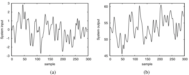
Example 1. The engine data set [19] was used to demonstrate the effectiveness of

the proposed OFS-LOO algorithm. The data were collected from a Leyland TL11 tur-bocharged, direct injection diesel engine operated at low engine speed, where the input u(t)was the fuel rack position and the outputy(t)was the engine speed. The input-output data set, depicted in Fig. 1, contained 410 samples. The first 210 data points were used in training and the last 200 points in model validation. The previous study

3.5 4 4.5 5 5.5 6

0 50 100 150 200 250 300 350 400

System input

sample

2.5 3 3.5 4 4.5 5

0 50 100 150 200 250 300 350 400

System output

sample

(a) (b)

Fig. 1. The engine data set: (a) inputu(t)and (b) outputy(t)

0.001 0.01 0.1

0 2 4 6 8 10 12 14 16 18 20

LOO mean square error

number of kernels

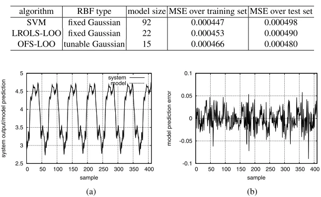
Table 1. Comparison of the three models obtained by the SVM, LROLS-LOO and OFS-LOO algorithms for the engine data set

algorithm RBF type model size MSE over training set MSE over test set

SVM fixed Gaussian 92 0.000447 0.000498

LROLS-LOO fixed Gaussian 22 0.000453 0.000490 OFS-LOO tunable Gaussian 15 0.000466 0.000480

2.5 3 3.5 4 4.5 5

0 50 100 150 200 250 300 350 400

system output/model prediction

sample system

model

-0.1 -0.05 0 0.05 0.1

0 50 100 150 200 250 300 350 400

model prediction error

sample

(a) (b)

Fig. 3. Modelling performance for the engine data set by the 15-node RBF network constructed by the OFS-LOO algorithm: (a) the model outputyˆksuperimposed on the system outputyk, and

(b) the modelling errorek=yk−yˆk

[9],[10] has shown that this data set can be modelled adequately asyi =fs(xi) +ei withyi=y(i),xi= [y(i−1)u(i−1)u(i−2)]T, wherefs(•)describes the unknown underlying system to be identified andeidenotes the system noise.

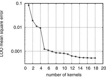
In the work [10], various state-of-the-art RBF and kernel modelling techniques were applied to construct Gaussian RBF network models for this data set, and the LROLS-LOO algorithm produced the best result. We applied the proposed OFS-LROLS-LOO technique to this data set. Fig. 2 depicts the LOO mean square error (MSE) as a function of the model size during the modelling process using the OFS-LOO. It can be seen that the algorithm automatically constructed a 17-term RBF model, sinceJ18 > J17. The LROLS-LOO algorithm was then employed to further simplify this obtained model, yielding a final 15-term RBF network. This 15-term model is compared with the model quoted from [10], which was obtained purely by the LROLS-LOO method, in Table 1. As a comparison, the model obtained by the SVM algorithm is also listed in Table 1. Fig. 3 illustrates the modelling performance of the 15-node RBF network constructed by the OFS-LOO algorithm.

Example 2. This example constructed a model for the gas furnace data set (Series J

-3 -2 -1 0 1 2 3

0 50 100 150 200 250 300

System input

sample

45 50 55 60

0 50 100 150 200 250 300

System output

sample

(a) (b)

Fig. 4. The gas furnace data set: (a) inputu(t)and (b) outputy(t)

Table 2. Comparison of the three models obtained by the SVM, LROLS-LOO and OFS-LOO algorithms for the gas furnace data set

algorithm RBF type model size training MSE LOO MSE SVM fixed Gaussian 62 0.052416 0.054376 LROLS-LOO fixed thin-plate-spline 28 0.053306 0.053685 OFS-LOO tunable Gaussian 15 0.054306 0.054306

0.1 1 10

0 2 4 6 8 10 12 14 16 18

LOO mean square error

number of kernels

Fig. 5. The LOO mean square error as a function of the model size for the gas furnace data set

study [10], several existing RBF modelling techniques were applied to this data set using the thin-plate-spline basis functions defined by

K(x−xi) =x−xi2log (x−xi), 1≤i≤N, (18)

45 50 55 60

0 50 100 150 200 250 300

system output/model prediction

sample system

model

-1 -0.5 0 0.5 1

0 50 100 150 200 250 300

model prediction error

sample

(a) (b)

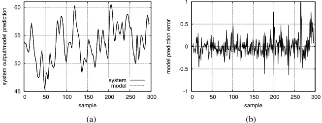
Fig. 6. Modelling performance for the gas furnace data set by the 15-node RBF network con-structed by the OFS-LOO algorithm: (a) the model outputˆyksuperimposed on the system output yk, and (b) the modelling errorek=yk−yˆk

We applied the proposed OFS-LOO technique to this data set. Fig. 5 depicts the LOO MSE as a function of the model size during the modelling process using the OFS-LOO. It can be seen that the algorithm automatically constructed a 16-term RBF model, sinceJ17 ≥ J16. The LROLS-LOO algorithm was then employed to further simplify this obtained model, yielding a final 15-term RBF network. This 15-term model is compared with the two models obtained by the SVM and LROLS-LOO algorithms, in Table 2. Fig. 6 illustrates the modelling performance of this 15-node RBF network constructed by the OFS-LOO algorithm.

4

Conclusions

A novel construction algorithm has been proposed for RBF networks with tunable nodes. Unlike most of the sparse RBF or kernel modelling methods, the RBF centres are not restricted to the training input data points and each node has an individually ad-justed diagonal covariance matrix. The proposed OFS-LOO method appends the RBF nodes one by one by incrementally minimising the LOO mean square error. This con-struction process is computationally efficient due to the orthogonalisation procedure employed. Moreover, the model construction is fully automatic and the user does not need to specify a termination criterion.

Acknowledgements

S. Chen wish to thank the support of the United Kingdom Royal Academy of Engineering.

References

2. Whitehead, B.A., Choate, T.D.: Evolving Space-Filling Curves to Distribute Radial Basis Functions Over an Input Space. IEEE Trans. Neural Networks 5 (1994) 15–23

3. Yang, Z.R., Chen, S.: Robust Maximum Likelihood Training of Heteroscedastic Probabilistic Neural Networks. Neural Networks 11 (1998) 739–747

4. Moody, J., Darken, C.J.: Fast Learning in Networks of Locally-Tuned Processing Units. Neural Computation 1 (1989) 281–294

5. Chen, S., Billings, S.A., Grant, P.M.: Recursive Hybrid Algorithm for Non-linear System Identification Using Radial Basis Function Networks. Int. J. Control 55 (1992) 1051–1070 6. Chen, S.: Nonlinear Time Series Modelling and Prediction Using Gaussian RBF Networks

with Enhanced Clustering and RLS Learning. Electronics Letters 31 (1995) 117–118 7. Chen, S., Cowan, C.F.N., Grant, P.M.: Orthogonal Least Squares Learning Algorithm for

Radial Basis Function Networks. IEEE Trans. Neural Networks 2 (1991) 302–309

8. Chen, S., Wu, Y., Luk, B.L.: Combined Genetic Algorithm Optimisation and Regularised Orthogonal Least Squares Learning for Radial Basis Function Networks. IEEE Trans. Neural Networks 10 (1999) 1239–1243

9. Chen, S., Hong, X., Harris, C.J.: Sparse Kernel Regression Modelling Using Combined Lo-cally Regularized Orthogonal Least Squares and D-Optimality Experimental Design. IEEE Trans. Automatic Control 48 (2003) 1029–1036

10. Chen, S., Hong, X., Harris, C.J., Sharkey, P.M.: Sparse Modelling Using Orthogonal For-ward Regression with PRESS Statistic and Regularization. IEEE Trans. Systems, Man and Cybernetics, Part B 34 (2004) 898–911

11. Vapnik, V.: The Nature of Statistical Learning Theory. Springer-Verlag, New York (1995) 12. Gunn, S.: Support Vector Machines for Classification and Regression. Technical Report, ISIS

Research Group, Department of Electronics and Computer Science, University of Southamp-ton, UK (1998)

13. Chen, S.S., Donoho, D.L., Saunders, M.A.: Atomic Decomposition by Basis Pursuit. SIAM Review 43 (2001) 129–159

14. Tipping, M.E.: Sparse Bayesian Learning and the Relevance Vector Machine. J. Machine Learning Research 1 (2001) 211–244

15. Sch¨olkopf, B., Smola, A.J.: Learning with Kernels: Support Vector Machines, Regulariza-tion, OptimizaRegulariza-tion, and Beyond. MIT Press, Cambridge, MA (2002)

16. Vincent, P., Bengio, Y.: Kernel Matching Pursuit. Machine Learning 48 (2002) 165–187 17. Lanckriet, G.R.G., Cristianini, N., Bartlett, P., Ghaoui, L.E., Jordan, M.I.: Learning the

Ker-nel Matrix with Semidefinite Programming. J. Machine Learning Research 5 (2004) 27–72 18. Chen, S., Wang, X.X., Harris, C.J.,: Experiments with Repeating Weighted Boosting Search

for Optimization in Signal Processing Applications. IEEE Trans. Systems, Man and Cyber-netics, Part B 35 (2005) 682–693

19. Billings, S.A., Chen, S., Backhouse, R.J.: The Identification of Linear and Non-linear Models of a Turbocharged Automotive Diesel Engine. Mechanical Systems and Signal Processing 3 (1989) 123–142