Testing explosive bubbles with time varying volatility

(1)

Testing explosive bubbles with time-varying

volatility

David I. Harvey, Stephen J. Leybourne and Yang Zu

University of Nottingham

July 2018

Abstract

This paper considers the problem of testing for an explosive bubble in …nancial data in the presence of time-varying volatility. We propose a weighted least squares-based variant of the Phillips, Wu and Yu (2011) test for explosive autoregressive behaviour. We …nd that such an approach has appealing asymptotic power proper-ties, with the potential to deliver substantially greater power than the established based approach for many volatility and bubble settings. Given that the OLS-based test can outperform the weighted least squares-OLS-based test for other volatility and bubble speci…cations, we also suggested a union of rejections procedure that succeeds in capturing the better power available from the two constituent tests for a given alternative. Our approach involves a nonparametric kernel-based volatility function estimator for computation of the weighted least squares-based statistic, together with the use of a wild bootstrap procedure applied jointly to both individ-ual tests, delivering a powerful testing procedure that is asymptotically size-robust to a wide range of time-varying volatility speci…cations.

Keywords: Rational bubble; Explosive autoregression; Time-varying volatility; Weighted least squares; Right-tailed unit root testing.

JEL Classi…cation: C12; C14, C22.

(2)

1 Introduction

Empirical identi…cation of explosive behaviour in …nancial asset price series is closely re-lated to the study of rational bubbles, with a rational bubble deemed to have occurred if explosive characteristics are manifest in the time path of prices, but not for the dividends. Consequently, methods for testing for explosive time series behaviour have been a focus of much recent research. In a now seminal paper, Phillips et al. (2011) [PWY] model poten-tial bubble behaviour using an explosive autoregressive speci…cation, and suggest testing for such a property using the supremum of a sequence of forward recursive right-tailed Dickey-Fuller unit root tests. The test has been widely applied, and has also prompted the development of related test procedures, such as those of Homm and Breitung (2012) who consider a supremum of backward recursive Chow-type Dickey-Fuller statistics, and Phillips et al. (2015) who consider a double supremum of forward and backward recursive statistics.

While these original papers assumed constant unconditional volatility in the under-lying error process, in practice time-varying, typically nonstationary, volatility is a well-known stylised fact observed in empirical …nancial data. Harvey et al. (2016) [HLST] demonstrate that the asymptotic null distribution of the PWY test depends on the nature of the volatility, and if the test is implemented using critical values derived under a ho-moskedastic error assumption, size is not controlled for nonstationary volatility patterns. This raises the possibility of misleading inference when using the standard PWY test in the presence of time-varying volatility, with the potential for spurious identi…cation of a bubble. HLST propose a wild bootstrap implementation of the PWY test, which ensures correct asymptotic size in the presence of time-varying volatility. This procedure also retains the same local asymptotic power as the original PWY test, if the latter were to be infeasibly size-corrected to account for the volatility pattern.

The PWY test and its related variants discussed above are all fundamentally based on OLS estimation of the underlying autoregression. In the context of time-varying volatility in the model errors, it is natural to consider whether a GLS-type transformation can deliver a more powerful testing approach. In this paper, we focus on this possibility, developing tests based on Dickey-Fuller unit root statistics derived from a weighted least squares [WLS] transformation of the model, along the lines of the approach considered by Boswijk and Zu (2015) in the context of full-sample testing for a unit root against a left-tailed stationary alternative.1 Speci…cally, we propose a PWY-type test, based on the supremum of a sequence of forward recursive statistics, but where the OLS-based Dickey-Fuller statistic is replaced by a WLS-based equivalent.

We begin by treating the volatility path as known, and demonstrate that our WLS-1_{See also Xu and Phillips (2008) and Xu and Yang (2015) for using similar kernel-type GLS corrections}

(3)

based test can o¤er substantially greater local asymptotic power than the PWY procedure for many volatility patterns and bubble speci…cations. This positive result suggests that the WLS-based approach merits development, o¤ering the potential to improve our ca-pacity to detect explosive autoregressive behaviour. Despite these potential large gains in local asymptotic power, we …nd that for certain volatility and bubble settings, the power rankings of the tests can be reversed, hence the PWY test can still o¤er a valuable role in bubble detection. In order to capture the relative power advantages of both tests across di¤erent volatility patterns, we then proceed to consider a union of rejections approach (cf. Harvey et al. (2009)), whereby the null is rejected in favour of explosive behaviour if either the WLS-based test or the PWY test rejects, subject to a scaling applied to the asymptotic critical values to ensure correct size of the composite procedure. We …nd that the union of rejections testing strategy performs very well across the range of volatility and bubble speci…cations that we consider.

Calculation of the WLS-based test statistic requires the volatility at each point in time, which is of course unknown in practice. To render the statistic feasible, we employ a nonparametric kernel-based volatility function estimator, and we show that substitution of this estimator in place of the true volatility path results in a statistic with the same limiting null and local alternative distributions as for the infeasible statistic. In common with the PWY statistic, our feasible WLS-based statistic has a limiting null distribution that depends on the volatility path. Following HLST, we suggest a wild bootstrap im-plementation of the test to achieve an asymptotically size-controlled procedure. For the union of rejections procedure, we then apply both the wild bootstrap HLST variant of PWY, and the wild bootstrap version of our WLS-based test. In order to ensure that the bootstrap-based union of rejections procedure is asymptotically correctly sized, we im-plement the wild bootstrap procedure to the two statisticsjointly, and also calculate the required critical value scaling constant from the wild bootstrap algorithm. We demon-strate the asymptotic validity of the joint procedure, showing that the local asymptotic power pro…les coincide with those for the infeasible case where the volatility is treated as known. Note that while we concentrate on introducing the techniques of this paper in the context of the PWY test, which is the prototype for the recent literature on recursive testing for bubbles, it should be noted that the methods we develop in principle apply more widely, e.g. to the double supremum extension by Phillips et al. (2015). We discuss this issue brie‡y in the …nal section of the paper.

(4)

section 4, and its asymptotic properties established. Finite sample properties of the tests are explored by Monte Carlo simulation in section 5, and an empirical example is provided in section 6 using FTSE and S&P 500 data. Section 7 discusses possible extensions of the current methodology and concludes the paper. Proofs of the results are given in the Appendix.

2 The bubble model and tests

2.1 The model

We will consider the following model with time-varying volatility for a time series _fytg,

t= 1; :::; T:

yt = +xt (1)

xt = (1 + t)xt 1+ut; t= 2; :::; T (2)

ut = t"t (3)

with x1 = Op(1). We make the following assumptions regarding the error "t in (3) and

the error standard deviation at timet, t:

A1 E("tjFt 1) = 0, E("2tjFt 1) = 1 with Ft the natural …ltration generated by fusgs 1,

and E("4

t)<1.

A2 t = (t=T), where (:) is a strictly positive function with (:) 2D[0;1], the space

of right continuous with left limit (càdlàg) processes on[0;1].

Under Assumption A1, "t is a martingale di¤erence sequence, and is hence

condition-ally …rst order uncorrelated, cf. Xu and Phillips (2008). Note that for empirical …nancial data, such an assumption is standard, where any admitted dependence is typically in the second moment (i.e. in the volatility). Assumption A2 implies that the innovation vari-ance is non-stochastic, bounded and displays a countable number of jumps, cf. Cavaliere and Taylor (2007), allowing for a very wide range of volatility dynamics.

For the time-varying autoregressive parameter (1 + _t) in (2) we adopt the following speci…cation:

t=

(

0 t= 2; : : : ;[ T] c=T t= [ T] + 1; : : : ; T

where [:] denotes the integer part of its argument. When c > 0, yt follows a unit root

(5)

behaviour with unit root dynamics up to a particular point in the sample, after which a bubble originates and explosive behaviour is manifest. Extensions to the case where the bubble terminates in-sample (with or without some form of collapse) could easily be entertained; see, for example, Harvey et al. (2017).

To test for the presence of a bubble, we consider a null hypothesis _H0 :c= 0 against the alternative_H1 :c >0. Under the null and local alternative, we can make use of the following invariance principle, which holds under Assumptions A1 and A2:

T 1=2

brTc

X

t=2

ut)

Z r

0

(s)dW(s)

where ₎denotes weak convergence and W(r) is a standard Brownian motion process.

2.2 A weighted least squares-based test

PWY propose a test for a bubble based on the supremum of recursive right-tailed Dickey-Fuller tests, based on OLS estimation. In view of the heteroskedasticity present in our model, it is natural to consider whether a GLS-type transformation can deliver a more powerful testing approach. Consequently, we now consider Dickey-Fullert-statistics based on a WLS transformation of the model, initially for the infeasible case where the t are

assumed known. Considering …rst the underlyingxtprocess in (2), the transformed model

can be written as

xt

t

= _txt 1

t

+"t; t= 2; : : : ; T: (4)

Here, (4) is an infeasible homoskedastic regression model of _f xt= tg on fxt 1= tg,

with coe¢ cient _t. Assuming knowledge of xt and t, a bubble test statistic could be

constructed using a sequence of WLS-based Dickey-Fuller regressions, analogous to the PWY OLS-based test statistic. In practice we do not observe xt, but yt = +xt as in

(1). In order to achieve invariance to , we simply replacextin (4) byy~t=yt y1, which

is equivalent to GLS-demeaning of yt in the sense of Elliott et al. (1996) using = 1 in

their notation, so that y1 becomes the estimator of . Our infeasible test statistic that assumes knowledge of t can then be written as

supBZ = sup

2[ 0;1]

BZ (5)

whereBZ denotes the Dickey-Fuller statistic calculated over the sub-sample_fy1; : : : ; y[ T]g, that is

BZ =

P[ T]

t=2 y~ty~t 1=

2

t

P[ T]

t=2 y~

2

t 1= 2t

(6)

In (5), the minimum sample length admitted in the sequence of sub-sample regressions is

[ 0T]. Note that the full-sample statistic BZ1 coincides with the infeasible test statistic considered in Boswijk and Zu (2015) in the context of left-tailed unit root testing against a stationary alternative.

The following theorem gives the limit distribution of supBZ: Theorem 1. Under _H1 and Assumptions A1 and A2,

supBZ₎ sup

2[ 0;1]

Lc( ) =MBZc

where

Lc( ) =

8 > < > :

R

0 Vc(r)dW(r)

(R0 Vc(r)2dr)

1=2 6

R

0 Vc(r)dW(r)+c

R

Vc(r)2dr

(R0 Vc(r)2dr)

1=2 >

with Vc(r) =Uc(r)= (r) and

Uc(r) =

( Rr

0 (s)dW(s) r6

ec(r )R

0 (s)dW(s) +

Rr

ec(r s) _(s)dW_(s) _{r >} :

Remark 1. The null limit distribution ofsupBZis obtained from the result in Theorem 1 simply by setting c = 0, so that supBZ ₎ _MBZ

0 . Of course, the limit distribution under both the null and local alternative depends on (r), hence the critical values and local asymptotic power function will be contingent on the volatility pattern present in the innovations.

We now proceed to evaluate the local asymptotic power of the supBZtest, comparing it to the local power of an infeasibly size-corrected PWY test. The PWY statistic follows a similar form to supBZ, but is based on the supremum of the t-ratios associated with

^ _{in the …tted OLS regressions}

yt= ^ + ^ yt 1+ ^et; t = 2; : : : ;[ T]

for ₂ [ 0;1]. Denoting this statistic by supDF, then under H1 and Assumptions A1 and A2, it can be shown from the results in Harvey et al. (2016) that

supDF ₎ sup

2[ 0;1]

Jc( ) =MDFc

where

Jc( ) =

8 > < > :

R

0 U~c(r)dUc(r)

( 1R

0 (r)2dr

R

0 U~c(r)2dr)

1=2 6

R

0 U~c(r)dUc(r)+c

R _~

Uc(r)2dr

( 1R

0 (r)2dr

R

0 U~c(r)2dr)

(7)

with U~c(r) =Uc(r) 1

R

0 Uc(s)ds, and where Uc(r) is as de…ned in Theorem 1. The null limit distribution for supDF is obtained on setting c = 0, so that supDF ₎ _MDF

0 . As with the result forsupBZ, the limit distribution under both the null and local alternative depends on (r). For the purposes of comparing local power with supBZ, we treat the volatility path as known, and compute infeasibly size-adjusted local asymptotic powers for a given (r).

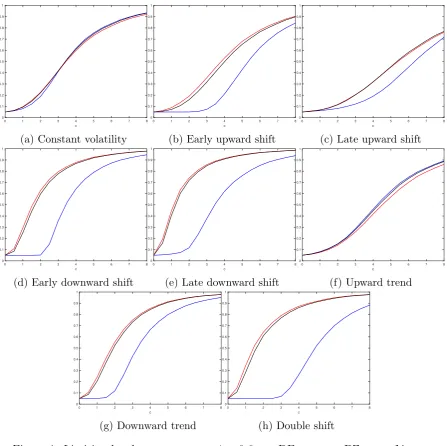
For the local power simulations, we consider the following volatility speci…cations for

(r), where_I(:)denotes the indicator function:

(a) Constant volatility: (r) = 1 ₈r.

(b) Early upward shift: (r) = 1 + 5_I(r 0:3). (c) Late upward shift: (r) = 1 + 5_I(r 0:8). (d) Early downward shift: (r) = 1 + 5_I(r <0:3).

(e) Late downward shift: (r) = 1 + 5_I(r <0:8). (f) Upward trend: (r) = 1 + 5r.

(g) Downward trend: (r) = 6 5r.

(h) Double shift: (r) = 1 + 5_I(0:4< r60:6).

Here, (a) is the benchmark homoskedastic case, while (b)-(e) specify one-o¤ variance shifts, (h) a double shift, and (f)-(g) linearly trending variances.

In Figures 1-2, we plot the asymptotic local power functions of supBZ and supDF, simulating the limit distributions _MBZc and MDFc using 10,000 Monte Carlo replications,

and approximating the Brownian motion processes in the limiting functionals using

N IID(0;1) random variates, with the integrals approximated by normalized sums of 1,000 steps. Here and throughout the paper, we set 0 = 0:1, as in PWY. Figures 1 and 2 report results for the bubble timings = 0:6 and = 0:8, respectively, under each volatility pattern, using a grid of cvalues from 0-8 in Figure 1 and 0-20 in Figure 2. For each test, power is evaluated using the 0.05-level null critical value appropriate for each volatility speci…cation (i.e. from_MBZ

(8)

powerful than supDF. Turning to the later bubble timing of Figure 2 ( = 0:8), the power gains for supBZ over supDF remain evident in most cases, with the gains again being substantial in cases (b), (d), (e), (g) and (h). As in Figure 1, the tests have broadly similar power levels under homoskedasticity, while for an upward trend (f) and now also a late upward shift (c), we see that supDF outperforms supBZ, albeit to a lesser degree than in the cases wheresupBZ outperforms supDF.

2.3 A union of rejections testing procedure

As neither test is dominant across all volatility speci…cations, we can consider employing a

union of rejections strategy along the lines of Harvey et al. (2009). These authors suggest such an approach in the context of combining inference from two unit root tests, one of which permits a linear trend in its deterministic speci…cation, the other of which excludes the trend, the idea being to harness the better power of the two when the presence of a trend is uncertain. The same principle can be used here, combining inference fromsupBZ

and supDF in the presence of uncertainty over the volatility speci…cation, in an attempt to capitalize on the relative power advantages of each across di¤erent volatility patterns. Speci…cally, denoting the asymptotic level null critical values of supDF and supBZ

(i.e. from _MDF0 and MBZ0 ) by qDFand qBZ, respectively, a union of rejections strategy can be written as the decision rule

Reject_H0 if fsupDF> qDFor supBZ> qBZg

where is a scaling constant chosen so that this decision rule yields an asymptotic size of under _H0. De…ning a single statistic _U as

U = max supDF;q

DF

qBZ supBZ

!

the decision rule is then equivalent to

RejectH0 if U > qDF:

Using the asymptotic results of the previous section, an application of the continuous mapping theorem (CMT) establishes that

U )max _MDF_c ;q

DF

qBZM BZ

c

!

:

The scaling constant can easily be determined from the limit distribution of _U with

(9)

qDF_=qBZ_{, all we require is the critical value} _qDF_{, which we denote} _qU_{. This can be}

obtained directly from the null limit distribution of_U. Finally, notice that since qDF _and

qBZ _{depend on the particular form of volatility speci…ed by} _(r)_{, so too will the critical} valueqU_{. At this point therefore,}_U_{, along with}_supDF_and_supBZ_{, is an infeasible testing}

procedure.

Along with the infeasible size-adjusted local asymptotic powers ofsupBZand supDF, Figures 1 and 2 show the corresponding power of the union of rejections procedure _U. We see throughout that the power pro…le of_U is always very similar to whichever pro…le of supDF and supBZ obtains the higher power. There is at worst only a small de…cit compared with the better of the two, suggesting that the union procedure is performing well here.

Thus far we have considered only the large sample properties of an infeasible variant of supBZ that is based on knowledge of the volatility function t. For any practical

implementation, construction of supBZ will require estimation of t. We address this

issue in the next section.

3 Nonparametric kernel estimation of the volatility

function and the feasible supBZ statistic

For estimation of 2

t we employ a simple nonparametric kernel smoothing estimator of

the form

^2_t =

PT

i=2Kh

i t

T ( yi)

2

PT

i=2Kh

i t T

(6)

where Kh(s) = K(s=h)=h and K(:) is a kernel function with bandwidth parameter h.

Based on ^2_t, a feasible version of BZ is then given by

BZ =

P[ T]

t=2 y~ty~t 1=^

2

t

P[ T]

t=2 y~t2 1=^

2

t

1=2

where, to economize on notation, we have rede…ned BZ , and we rede…ne supBZ analo-gously. To derive the asymptotic distribution of supBZ, in addition to A1 and A2, we make the following further assumptions:

A3 "t follows a symmetric distribution, and E("8t)<1.

A4 (:) is a Lipschitz continuous function on[0;1].

A5 K(:)is a bounded nonnegative function de…ned on the real line andR1₁K(r)dr = 1. A6 As T _{! 1},h_!0 and T h2

(10)

The assumption E("8

t) < 1 in A3 is also used in Xu and Phillips (2008). The

symmetry assumption for "t in A3 is made for technical reasons, and is usually easily

satis…ed for the kind of equity or equity index returns considered in this paper. The continuity assumption in A4 is used for ease of exposition and could be relaxed to allow for a …nite number of discontinuities using the strategy in Xu and Phillips (2008), thereby incorporating examples of volatility speci…cations involving jumps, such as the shifts in volatility cases of section 2.2. From a modelling perspective, large movements in the volatility can be incorporated in the Lipschitz continuous assumption as well; see Boswijk and Zu (2015) for related discussions. The assumption on the volatility function is nonparametric and can allow for a wide range of volatility dynamics such as trending volatility, (multiple) smooth transition (e.g. logistic) changes in variance, or volatility with Fourier-form periodicity. Our assumption A5 on the kernel function is more general than the Xu and Phillips leave-one-out kernel, and is also more general than the truncated kernel considered in Boswijk and Zu (2015), while the rate condition in A6 coincides with Xu and Phillips (2008).

The following theorem gives the limit distribution of the feasible version of supBZ: Theorem 2. Under _H1 and Assumptions A1-A6

supBZ₎_MBZ_c :

Remark 2. The feasible statisticsupBZhas the same limiting properties as its infeasible counterpart.

The remaining issue that pertains to a full feasible application of supBZ, supDF and hence _U, is that the appropriate asymptotic null critical valuesqBZ _and _qDF _{arising from}

MBZ

0 andMDF0 depend on the volatility function (s). In the context ofsupDF, Harvey et al. (2016) employ a wild bootstrap procedure to obtain asymptotically valid null critical values. We now show that this same approach can be employed for supBZand _U.

4 A wild bootstrap procedure

Following Harvey et al. (2016), our wild bootstrap algorithm is de…ned as follows:

1. Generate a wild bootstrap sample _fyb

tgTt=1 by setting

yb₁ = 0; y_tb =y_tb ₁+ ytzt; t= 2; ::; T

where the zt areiid standard normal variates.

(11)

3. Repeat step 1 and step 2 M times, denoting the resulting pairs of statistics by fsupDFb₁;supBZb_1g; :::;_fsupDFb_M;supBZb_M_g.

Theorem 3. Under _H1 and Assumptions A1-A6

supDFb_m supBZb_m

!

p

) M

DF 0

MBZ0

!

jointly, for any 1 m M, where ₎p denotes weak convergence in probability.

Remark 3. The results of Theorem 3 shows that the wild bootstrap procedure is …rst order valid in approximating the asymptotic null distributions of the supDF and supBZ

statistics under _H1 (which includes H0 as a special case). The asymptotic validity of the marginal bootstrap supDF statistic is shown in Harvey et al. (2016). Theorem 3 strengthens their results with the marginal convergence of the bootstrap supBZstatistic and their joint convergence. The joint convergence occurs because both statistics are calculated from the same bootstrap sample; this result is needed for the validity of the union test strategy.

The level bootstrap critical values are obtained from the empirical distribution func-tions of supDFb_m and supBZb_m calculated fromM bootstrap replications. Denoting these critical values asqb;DF andqb;BZ, a rejection of_H0 forsupDFis obtained if supDF> qb;DF and a rejection of _H0 for supBZ is obtained if supBZ> qb;BZ. As T; N ! 1, it follows thatqb;DF andqb;BZ converge in probability toqDF_and_qBZ_;_{so these bootstrap procedures} are correctly sized in the limit under _H0, and inherit exactly the same asymptotic local power functions under _H1 as their infeasibly size-corrected counterparts in section 2.2.

The wild bootstrap counterpart of the union statistic _U is given by

Umb = max supDF b

m;

qb;DF

qb;BZ supBZ

b m

!

form = 1; :::; M. The results in Theorem 3, and an application of the continuous mapping theorem (CMT), veri…es that

Umb p

)max _MDF₀ ;q

DF

qBZM BZ 0

!

:

The level bootstrap critical value for the union is obtained from the empirical distribu-tion funcdistribu-tion of _Ub

m, and denoting this critical value as q

b;U _{we reject}

H0 when U > qb;U, where

U = max supDF;q

b;DF

qb;BZ supBZ

!

(12)

Remark 4. Notice that this is a feasible variant of_U which is based on replacingqDF_=qBZ with qb;DF=qb;BZ.

As T; N _{! 1}, _U is correctly sized in the limit under _H0, since qb;U converges in probability to qU_{, and also obtains the same asymptotic local power function under} _H

1 as the infeasibly size-corrected version in section 2.2.

We have therefore established asymptotic validity of bootstrap variants of supDF,

supBZ and _U in terms of size control and local power. We now turn to a comparison of the …nite sample properties of these procedures.

5 Finite sample properties

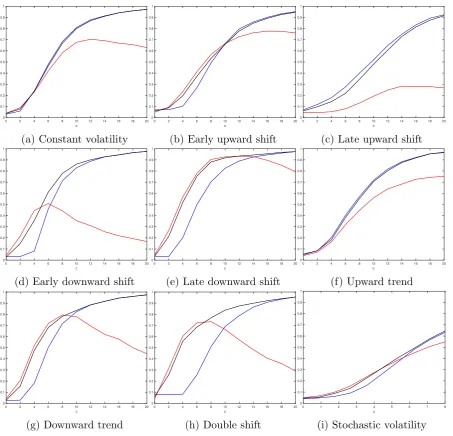
Our …nite sample simulations are based on (1)-(3) with T = 200. Here we set = 0

and x1 = 0, with the "t are generated as N IID(0;1) random variates. Figures 3 and 4

show 0.05-level …nite sample sizes and powers for the same settings of as used in the asymptotic simulations of Figures 1 and 2, respectively, with the …nite sample volatility functions t being the discrete time analogues of those given in cases (a)-(h) of section

2.2. Here we use 1,000 Monte Carlo replications, together with M = 499 bootstrap replications.

For the volatility estimates ^2_t we employ the Gaussian kernel

K(r) = _p1

2 exp( r

2_=2):

We determine the bandwidthhusing a standard leave-one-out cross-validation bandwidth selection procedure. Speci…cally, for the cross-validation criteria de…ned by

CV(h) =

T

X

t=2

(( yt)2 ^2t; )

2

where ^2_t; is the Gaussian kernel-based variance estimator ^2_t that imposes K(0) = 0, the bandwidth is chosen as

hCV = arg min h2[hl;hu]

CV(h):

We then construct the ^2_t in (6) with hCV in place ofh.2

The …nite sample power curves corresponding to Figure 1 ( = 0:6) and Figure 2 ( = 0:8) are given in Figure 3 (a)-(h) and Figure 4 (a)-(h), respectively. The results

2_{In our implementation, we set} _h

l = 1=(2T) and hu = 1=6, which ensures that the interval of

(13)

for c = 0 (which are of course the same across Figures 3 and 4) show that the feasi-ble version of supBZ displays excellent size control for T = 200. The power curves of the bootstrapped tests in Figure 3 ( = 0:6) generally bear close resemblance to their asymptotic counterparts, with the exception of the late upward volatility shift (c) where the powers of supBZ appear lower than in the limit case. For (c) supBZ is now less powerful than supDF.

In Figure 4 ( = 0:8), we observe that supBZ demonstrates non-monotonicity in its power pro…les, with power reversals observed for the larger values of c (something not observed in Figure 3). We conjecture that this behaviour is due to large values of

c causing the estimates of ^2_t to become in‡ated via their dependence on yt = xt =

(c=T)xt 1 +ut, which in …nite samples is not necessarily a good proxy for ut unless T

is large relative to c. Despite this tendency for power reversals with supBZ, it is still the case that the power pro…le of _U is monotonic and again similar to whichever pro…le of supDF and supBZobtains the higher power, though obviously for large c, this pro…le is now typically that of supDFrather than supBZ, in contrast to what was typically observed in our asymptotic simulations. One noteworthy observation is that for the cases where supBZ displays non-monotonic power, _U can actually have power greater than either supDFor supBZ for certain intermediate c values around the intersection of the

supDFand supBZ power pro…les. It appears, therefore, that_U o¤ers a robust approach to testing, capturing most of the relatively high power that supBZcan o¤er over supDF

for small to moderate magnitude bubbles, while retaining high power across c in cases where the power of supBZ can drop relative to supDF.

Our model assumes a deterministic volatility function, however it is also of interest to evaluate the performance of the tests under stochastic volatility, which is not covered by assumption A2 but is of empirical relevance. The volatility model we simulate for this exercise is the so-called square root process

d 2(r) = 0:03(0:25 2(r))dr+ 0:1p 2_(r)dB(r)

where B(r)is a standard Brownian motion process, and the parameter settings used are representative of those considered in Bollerslev and Zhou (2002). The volatility model is re-simulated in each replication of the Monte Carlo experiment, using N IID(0;1)

drawings to approximate the Brownian motion increments, with these drawings being independent of those for"t. Figures 3 (i) and 4 (i) report the empirical rejection

(14)

present.3 _{As regards the power of the tests,} _supBZ _and _supDF _{tend to perform quite}

similarly under this stochastic volatility model, withsupBZdisplaying small power gains over supDF for smallc, and a reverse pattern for larger c.

6 Empirical illustrations

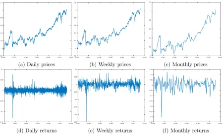
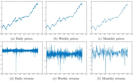
In this section, we apply the bootstrapsupDF,supBZand _U procedures to two data sets, with supBZ using the same Gaussian kernel and cross-validation bandwidth selection method discussed in section 5. The data are logarithms of the in‡ation-adjusted FTSE index from December 1985 to December 1999 and the S&P 500 index from January 1980 to March 2000. For each dataset we consider monthly, weekly and daily frequencies. Figure 5 and Figure 6 show the time series plots of log prices and the …rst di¤erences (log returns) for the FTSE index and the S&P 500 index, respectively, at the three sampling frequencies. We see that the levels of both series are generally increasing during the period considered (Homm and Breitung, 2012, consider similar sample periods so that the sample endpoints correspond to periods where the prices reach their peaks). From the plots of the …rst di¤erences (i.e. log returns), the presence of time varying volatility is clearly a plausible phenomenon.

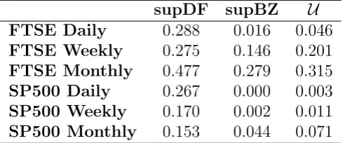
The three procedures supDF, supBZand _U are applied to each of the six series, with the results given in Table 1, the entries being bootstrapp-values associated with the dif-ferent procedures. First we observe that thesupDF test does not reject the null in favour of explosive behaviour for any of the series considered at conventional signi…cance levels.4

Turning to supBZ, we …nd evidence of explosive behaviour, at least at the 0.05-level, for the daily FTSE series and all frequencies of the S&P 500 index. These rejections are preserved when considering the_U procedure, albeit at a slightly weaker signi…cance level for monthly S&P 500. This pattern of results, where rejections are obtained by supBZ

and_U but notsupDF, …ts well with our asymptotic and …nite sample simulation …ndings when an explosive period of small to modest magnitude is present in the data, along with time-varying volatility. Given that the supDF test alone fails to detect these explosive episodes, our application reinforces our earlier …ndings that the WLS-based supBZ pro-cedure can o¤er enhanced levels of detectability of explosive behaviour. Moreover, given that the union of rejections procedure does not reduce the number of series for which rejections of the unit root null are found, we again …nd that there is little cost to adopt-ing this joint test approach, which also provides a degree of insurance for other potential cases where supDF might reject but supBZnot.

3_{This is not a surprising result, as the wild bootstrap method only mimics the heteroskedastic pattern}

in the data, but is unable to reproduce the dependence between the volatility process increments and the model errors.

4_{We also compared the}_supDF_{test statistic with standard critical values obtained under an assumption}

(15)

7 Discussion and conclusion

In this paper we have proposed a WLS-based variant of the PWY test for explosive autoregressive behaviour in a …nancial time series. We …nd that such an approach has appealing asymptotic power properties, with the potential to deliver substantially greater power than the established OLS-based approach for many volatility and explosive set-tings. Given that the OLS-based test can outperform the WLS-based test for other volatility and explosive speci…cations, we also suggested a union of rejections procedure that succeeds in capturing the better power available from the two constituent tests for a given alternative. Our approach involves a nonparametric kernel-based volatility function estimator for computation of the WLS-based statistic, together with the use of a wild bootstrap procedure applied jointly to both individual tests, delivering a powerful testing procedure that is asymptotically size-robust to a wide range of time-varying volatility speci…cations. Finite sample simulations indicate that the procedures should work well in practice, and application of the tests to FTSE and S&P 500 price data supports our premise that the WLS-based test can provide improved ability to detect explosive be-haviour compared to extant procedures.

While we have focused our attention on a PWY-type framework, using a single supre-mum of forward recursively calculated statistics, our WLS approach could of course be used in the context of the double supremum testing approach of Phillips et al. (2015). The WLS variant of their double supremum test statistic is given by

supBZ = sup

12[0;1 ]; 22[ 1+ ;1]

BZ 1; 2

where

BZ 1; 2 =

P[ 2T]

t=[ 1T]+1 y~ty~t 1=^

2

t

P[ 2T]

t=[ 1T]+1y~t2 1=^

2

t

1=2

withy~tand^2t as de…ned above. The wild bootstrap and union of rejections methodologies

can be applied tosupBZ in an entirely similar way as tosupBZ, and we would anticipate power gains to be available for these more general tests also.

Finally, the autoregressive speci…cation that we have adopted in this paper involves a one-time change from unit root to explosive dynamics. One could also consider a more general nonparametric speci…cation for t, along with an appropriate modi…cation to the

(16)

References

Bollerslev, T. and Zhou, H. (2002). Estimating stochastic volatility di¤usion using conditional moments of integrated volatility. Journal of Econometrics 109, 33–65.

Boswijk, H. P. and Zu, Y. (2018). Adaptive wild bootstrap testing for a unit root with nonstationary volatility. The Econometrics Journal, forthcoming, doi:10.1111/ ectj.12100.

Cavaliere, G. and Taylor, A.M.R. (2007). Testing for unit roots in time series models with non-stationary volatility. Journal of Econometrics 140, 919–947.

Elliott, G., Rothenberg, T.J. and Stock, J.H. (1996). E¢ cient tests for an autoregressive unit root. Econometrica 64, 813–836.

Harvey, D. I., Leybourne, S.J. and Sollis, R. (2017). Improving the accuracy of asset price bubble start and end date estimators. Journal of Empirical Finance 40, 121– 138.

Harvey, D. I., Leybourne, S.J., Sollis, R. and Taylor, A.M.R. (2016). Tests for explosive …nancial bubbles in the presence of non-stationary volatility. Journal of Empirical Finance 38, 548–574.

Harvey, D.I., Leybourne, S.J. and Taylor, A.M.R. (2009). Unit root testing in practice: dealing with uncertainty over the trend and initial condition (with commentaries and rejoinder). Econometric Theory 25, 587-667.

Homm, U. and Breitung, J. (2012). Testing for speculative bubbles in stock markets: a comparison of alternative methods. Journal of Financial Econometrics 10, 198–231.

Phillips, P.C.B., Shi, S.-P. and Yu, J. (2015). Testing for multiple bubbles: historical episodes of exuberance and collapse in the S&P 500. International Economic Review

56, 1043–1077.

Phillips, P.C.B., Wu, Y. and Yu, J. (2011). Explosive behavior in the 1990s Nasdaq: when did exuberance escalate stock values? International Economic Review 52, 201–226.

Robinson, P. M. (1987). Asymptotically e¢ cient estimation in the presence of het-eroskedasticity of unknown form. Econometrica 55, 875–891.

(17)

Xu, K.-L. and Phillips, P.C.B. (2008). Adaptive estimation of autoregressive models with time-varying variances. Journal of Econometrics 142, 265–280.

Xu, K.-L. and Yang, J.C. (2015). Towards uniformly e¢ cient trend estimation un-der weak/strong correlation and non-stationary volatility. Scandinavian Journal of Statistics, 42, 63-86.

Appendix: Proofs of theorems

In what follows, we set = 0 andy1 = 0, without loss of generality, so that yt = ~yt=xt.

Proof of Theorem 1

First notice that

BZ =

P[ T]

t=2

ytyt 1

2 t

P[ T]

t=2

y2

t 1

2 t

1=2:

Using the result

T 1=2y[rT])Uc(r)

which follows straightforwardly from Theorem 1 of Harvey et al. (2016), it follows that

T 1=2y[rT] 1

t )

Uc(r)= (r) =Vc(r):

Notice that this holds for all r ₂ (0;1) and the Uc (thus also Vc) process is de…ned to

have two regimes. One immediate consequence of this weak convergence result is that

T 2

[ T]

X

t=2

y2

t 1

2

t )

Z

0

Vc(r)2dr:

For yt= t, notice that

yt

t

=

(

"t 6

(c=T)yt 1

t +"t >

:

Then it follows easily that when 6 ,

T 1

[ T]

X

t=2

ytyt 1 2

t

)

Z

0

Vc(r)dW(r)

and so

BZ ₎

R

0 Vc(r)dW(r)

R

(18)

When > ,

T 1

[ T]

X

t=2

ytyt 1 2

t

= T 1

[ T]

X

t=2

"tyt 1

t

+T 1

[ T]

X

t=[ T]+1

(c=T)y2

t 1 2 t ) Z 0

Vc(r)dW(r) +c

Z

Vc(r)2dr

and so

BZ ₎

R

0 Vc(r)dW(r) +c

R

Vc(r)2dr

R

0 Vc(r)2dr

1=2 :

It then follows that, via the continuous mapping theorem,

supBZ₎ sup

2[ 0;1]

Lc( ) =MBZc :

Proof of Theorem 2

In order for thefeasible statisticBZ , in which 2

t is replaced by ^

2

t, to converge toLc( )

(the limit of its infeasible counterpart), we require the following two conditions to hold:

T 1

T

X

t=2

( ytyt 1=^2t) T

X

t=2

( ytyt 1= 2t)

!

= op(1) (7)

T 2

T

X

t=2

(yt 1=^t)2 T

X

t=2

(yt 1= t)2

!

= op(1): (8)

To show (7) and (8), we largely adapt the strategy used in Robinson (1987) and Xu and Phillips (2008).

For (7), …rst notice that the spot variance estimator can be written as

^2_t =

T

X

i=2

wt;iu^2i

where the weights are de…ned aswt;i =Kh i t_T =

PT

i=2Kh i t_T and satisfy

PT

i=2wt;i = 1.

De…ning ~2_t =PT_i₌₂wt;iu2i and 2t =

PT

i=2wt;i 2i, we can make the following

decomposi-tion:

T 1

T

X

t=2

ytyt 1(1=^2t 1= 2t) = T 1 T

X

t=2

ytyt 1(1=^2t 1=~2t) +T 1 T

X

t=2

ytyt 1(1=~2t 1= 2t)

+T 1

T

X

t=2

ytyt 1(1= 2t 1=

2

t)

(19)

show that all the three terms are op(1).

For A,

jA_j 6 max

t 1=(^

2

t~2t) T

X

t=2

( ytyt 1)(^2t ~2t)=T

6 max

t 1=(^

2

t~2t) T 2

T

X

t=2

( ytyt 1)2

!1=2 _T

X

t=2

(^2_t ~2_t)2

!1=2

using Cauchy-Schwartz inequality. Notice^2_t and ~2_t are bounded away from 0,maxt 1=^2t~

2

t

will at most be Op(1); also it is easy to obtain that T 2PT_t₌₂( ytyt 1)2 =Op(1). Then

to show A=op(1), we are left to showPT_t₌₂(^2t ~

2

t)2 =op(1). Now

^2_t ~2_t =

T

X

i=2

wt;i(^u2i u

2

i)

=

T

X

i=2

wt;i(( yi)2 ( i"i)2)

=

T

X

i=2

wt;i(( iyi 1 + i"i)2 ( i"i)2)

= Op(T 1) (9)

where in the last step we use the de…nition that _i = 0 before and _i =c=T after , so ^2_t ~2_t will be at mostOp(T 1). This further implies that

PT

t=2(^

2

t ~

2

t)2 =Op(T 1),

which completes the proof forA=op(1).

For B, notice that

B = T 1

T

X

t=2

ytyt 1(1=~2t 1=

2

t)

= T 1

T

X

t=2

ytyt 1( 2t ~

2

t)

4

t +T

1

T

X

t=2

ytyt 1( 2t ~

2

t)

2 4

t ~

2

t (10)

(20)

terms asB1and B2, and we look at them separately. For B1,

B1 = T 1

T

X

t=2

ytyt 1( 2t ~

2

t)

4

t

= T 1

T

X

t=2

( _tyt 1+ut)yt 1( 2t ~

2

t)

4

t

= cT 2

T

X

t=[ T]+1

y_t2 ₁( 2_t ~2_t) _t4+T 1

T

X

t=2

utyt 1( 2t ~

2

t)

4

t

= B11 +B12

where B11 and B12 are de…ned implicitly. Under the null B11 = 0, while under the alternative we have

jB11_j = cT 2

T

X

t=[ T]+1

y2_t ₁( 2_t ~2_t) _t4

6 Cmax

t (

2

t ~

2

t) T

2

T

X

t=[ T]+1

y2_t ₁

where _C generically denotes a positive constant. Notice that

P(max

t j~

2

t

2

tj> ") 6 T

X

t=2

P(_j~2_t 2_t_j> ")

6

T

X

t=2

E_j~2_t 2_t_j4="4 =Op 1=(T h2) (11)

and it is straightforward to show thatT 2PT

i=2y

2

ti 1 =Op(1), so we haveB11 =op(1)

be-cause T h2

! 1. For the termB12, …rst notice that utyt 1( 2t ~

2

t) t is a martingale

di¤erence sequence with respect to the …ltration_Ft. This is because

E utyt 1( 2t ~

2

t)

4

t jFt 1 = yt 1 t2E(utjFt 1) + t4E utyt 1

T

X

i=2

wiu2ijFt 1

!

= _t4E utyt 1

t 1

X

i=2

wiu2ijFt 1

!

+ _t4E utyt 1

T

X

i=t+1

wiu2ijFt 1

!

+ _t4E u3_tyt 1wtjFt 1

where the …rst term is clearly 0, the second term is also 0 by noticing that, for i > t,

(21)

while the third term is also 0 by the assumption that E(u3

tjFt 1) = 0.5 Using Markov’s inequality and the fact thatB12is a sum of a martingale di¤erence sequence we have

P(_jB12_j> ") = P T 1

T

X

t=2

ytyt 1( 2t ~2t) t4 > "

!

6 E T 1

T

X

t=2

ytyt 1( 2t ~

2 t) 4 t 2 ="2

6 CT 2

T

X

t=2

E_j ytyt 1j2( 2t ~

2

t)

2_="2

6 CT 2" 2

T

X

t=2

(E_j ytyt 1j4)1=2(E( 2t ~

2

t)

4₎1=2

6 max t E( 2 t ~ 2 t)

4 1=2

CT 2" 2

T

X

t=2

(E_j ytyt 1j4)1=2:

It is easy to see thatT 2PT

t=2(Ej ytyt 1j4)1=2 =Op(1), and we next show that maxtE( 2t

~2_t)4 ₌_o

p(1):

E( 2_t ~2_t)4 = E

T

X

i=2

wt;i(u2i

2 i) !4 6 E T X i=2

w_t;i2 (u2_i 2_i)2

!2

6 (1=T h)2E

T

X

i=2

wt;i(u2i

2

i)

2

!2

6 (1=T h)2

T

X

i=2

wt;iE(u2i

2

i)

4

= Op (1=T h)2 (12)

where in the second step Burkholder’s inequality for a martingale di¤erence sequence is used, in the third step the fact that maxiwt;i =O(1=(T h))is used, in the fourth step we

use Jensen’s inequality, and in the last step we use the boundedness of the 8th moment of "t from Assumption A3. So, we have shown B12 = op(1), which implies B1 = op(1).

For the term B2in (10),

T 1

T

X

t=2

ytyt 1( 2t ~

2

t)

2 4

t ~

2

t 6C T

2

T

X

t=2

( ytyt 1)2

!1=2 _T

X

t=2

( 2_t ~2_t)4

!1=2

:

5_{In Xu and Philips (2008), a leave-one-out estimator for spot volatility is used to make the third}

term 0. Here our assumption of a symmetric "t achieves the same result without the need to use the

(22)

As in the derivation of A = op(1), it is easy to see that T 2PT_t₌₂( ytyt 1)2 = Op(1).

Using the Markov inequality, it follows that

P

T

X

t=2

( 2_t ~2_t)4 > "

!

6 E

T

X

t=2

( 2_t ~2_t)4=" = Op(1=(T h2)) =op(1)

by applying the result in (12), and recalling the assumption that T h2

! 1, so we have

B2 = op(1). This completes the proof forB =op(1).

For C, notice that

C = T 1

T

X

t=2

ytyt 1(1= 2t 1= 2t)

= cT 2

T

X

t=[ T]+1

y_t2 ₁(1= 2_t 1= 2_t) +T 1

T

X

t=2

utyt 1(1= 2t 1=

2

t)

= C1 +C2

where C1and C2 are de…ned implicitly. For C1,

C1 = cT 2

T

X

t=[ T]+1

y_t2 ₁(1= 2_t 1= 2_t)

6 cmax

t

2

t 2t max

t

2

t 2t T 2

T

X

t=[ T]+1

y_t2 ₁:

HereT 2PT

t=[ T]+1y2t 1 =Op(1),maxtj t2 2tj=Op(1), and we next show thatmaxtj 2t 2tj=

o(1), as follows

2

t

2

t =

PT

i=2Kh i t_T 2i

PT

i=2Kh

i t T

2

t

=

Z 1 0

1 hK

s t=T

h (s)ds(1 +o(T

1₎₎ 2

t

=

Z 1 1

K(s)ds t(1 +o(T 1)) 2t =o(1) (13)

(23)

di¤erence sequence, so

E(C2)2 = E T 1

T

X

t=2

utyt 1(1= 2t 1=

2

t)

!2

= T 2

T

X

t=2

E[E(utyt 1)2jFt 1](1= 2t 1=

2

t)

2

= T 2

T

X

t=2

E(y_t2 ₁)( 2_t 2_t)2 _t4 _t2

6 (max

t j

2

t

2

tj)

2_max t 4 t 2 t T 2 T X t=2

E(y2_t ₁):

Clearly T 2PT

t=2E(y

2

t 1) =Op(1), and it su¢ ces to show maxtj 2t 2tj =op(1), which

is already shown in (13). We have thus shown that C2 =op(1) and alsoC =op(1).

For (8), notice that

T 2

T

X

t=2

(yt 1=^t)2 T

X

i=2

(yt 1= t)2 6CT 2 T

X

t=2

y_t2 _1j^2_t 2_t_j:

Since T 2PT

t=2y2t 1 =Op(1), for (8) to hold it su¢ ces to show

max

t j^

2

t

2

tj=op(1): (14)

First make the decomposition

max

t j^

2

t

2

tj6max_t j^

2

t ~

2

tj+ max_t j~

2

t

2

tj+ max_t j

2

t

2

tj=D+E+F

where the three terms are de…ned implicitly. For the term D, using the result in (9), it easily follows that D= Op(T 1). E =op(1) has already been shown in (11). F =o(1)

has already been shown in (13). We have thus shown (14). This completes the whole proof.

Proof of Theorem 3

The result for supDFb_m follows straightforwardly from Harvey et al. (2016). Also from Harvey et al. (2016), it follows that

T 1=2yb_[_rT_] ₎p

Z r

0

(24)

It then follows easily by the uniform consistency of the spot volatility estimator in (14), and since [rT]+1! (r), that

T 1=2y_[b_rT_]=^[rT]+1

p

)V0(r):

Application of the continuous mapping theorem then gives

[ T]

X

t=2

y_tbyb_t ₁=^2_t ₎p

Z

0

V0(r)dW(r) [ T]

X

t=2

y2_t ₁=^2_t ₎p

Z

0

V0(r)2dr:

Denoting byBZb theBZ statistic based on a bootstrap sample, we then obtain

BZb ₎p

R

0 V0(r)dW(r)

R

0 V0(r)2dr 1=2

and thus

(25)

0 1 2 3 4 5 6 7 8 c 0 0.1 0.2 0.3 0.4 0.5 0.6 0.7 0.8 0.9 1

(a) Constant volatility

0 1 2 3 4 5 6 7 8