A Dissertation by
SUJUNG CHOI
Submitted to the Office of Graduate Studies of Texas A&M University
in partial fulfillment of the requirements for the degree of DOCTOR OF PHILOSOPHY
August 2005
A Dissertation by
SUJUNG CHOI
Submitted to Texas A&M University in partial fulfillment of the requirements
for the degree of
DOCTOR OF PHILOSOPHY
Approved by:
Chair of Committee, Emanuel Parzen Committee Members, Bani Mallick
Michael Sherman David R. Larson Head of Department, Simon Sheather
August 2005 Major Subject: Statistics
ABSTRACT
On Two-Sample Data Analysis By Exponential Model. (August 2005) Sujung Choi, B.A., Yonsei University;
M.A., Yonsei University
Chair of Advisory Committee: Dr.Emanuel Parzen
We discuss two-sample problems and the implementation of a new two-sample data analysis procedure. The proposed procedure is based on the concepts of mid-distribution, design of score functions, components, comparison distribution, comparison density and exponential model. Assume that we have a random sample X1,· · · , Xm from a continuous distribution F(y) = P(Xi ≤ y), i = 1,· · · , m and a random sample Y1,· · · , Yn from a continuous distribution G(y) = P(Yi ≤ y), i = 1,· · · , n. Also as-sume independence of the two samples. The two-sample problem tests homogeneity of two samples and formally can be stated asH0 :F =G. To solve the two-sample prob-lem, a number of tests have been proposed by statisticians in various contexts. Two typical tests are the two-sample t−test and the Wilcoxon’s rank sum test. However, since they are testing differences in locations, they do not extract more information from the data as well as a test of the homogeneity of the distribution functions. Even though the Kolmogorov-Smirnov test statistic or Anderson-Darling tests can be used for the test of H0 : F = G, those statistics give no indication of the actual relation of F to G when H0 : F = G is rejected. Our goal is to learn why it was rejected. Our approach gives an answer using graphical tools which is a main property of our approach. Our approach is functional in the sense that the parameters to be esti-mated are probability density functions. Compared with other statistical tools for two-sample problems such as the t-test or the Wilcoxon rank-sum test, density
esti-mation makes us understand the data more fully, which is essential in data analysis. Our approach to density estimation works with small sample sizes, too. Also our methodology makes almost no assumptions on two continuous distributions F and G. In that sense, our approach is nonparametric. Our approach gives graphical el-ements in two-sample problem where exist not many graphical elel-ements typically. Furthermore, our procedure will help researchers to make a conclusion as to why two populations are different when H0 is rejected and to give an explanation to describe the relation between F and Gin a graphical way.
ACKNOWLEDGEMENTS
Graduate study in the Department of Statistics at Texas A&M means a lot to me. I have spent a fifth of my life here and learned so many precious things about statistics and life. In this respect, I am indebted to many of the faculty of the Department of Statistics, not only for discussions related to this dissertation but also for their time and effort while teaching the several courses I attended. In this regard, I would like to thank Professor Bani Mallick, Professor Michael Sherman and Professor David Larson from whom I learned much.
My advisor, Professor Manny Parzen is a great scholar and philosopher. It was a great opportunity for me to work with him. From him, I learned philosophy and attitude on research as well as knowledge of statistics. Also, he trained me to be a statistician with his great vitality and intelligence. He spared no pains to give all the detailed comments on my dissertation which greatly improved my dissertation. I really appreciate what he has done for me. Also, I want to give my special thanks to Professor Michael Longnecker and Marilyn Randall who have been taking care of all necessary documents to maintain my student status. Without their help, it would have been difficult to concentrate on my study in the states.
This work would never have been done without understanding, love and support of my family in Korea. In any situations, they supported my study and believed in me. Since I know that it was not always easy for them, I would like to express my appreciation from the bottom of my heart. Also, there are friends who helped me in several ways here, in College Station. I would like to express my special thanks to them since they made me feel relaxed whenever I was under great stress. After all, I could not have completed this work without other people’s help.
TABLE OF CONTENTS
CHAPTER Page
ABSTRACT . . . iii
ACKNOWLEDGEMENTS . . . vi
TABLE OF CONTENTS . . . vii
LIST OF TABLES . . . ix
LIST OF FIGURES . . . x
CHAPTER I INTRODUCTION. . . . 1
1.1. The Two-Sample Problem . . . 1
1.2. Outline of This Dissertation . . . 3
II COMPARISON DISTRIBUTION FUNCTION AND COMPARISON DENSITY FUNCTION . . . . 4
2.1. Introduction . . . 4
2.2. Population Concepts . . . 4
2.3. Sample Comparison Distribution and Comparison Den-sity Functions . . . 12
III EXPONENTIAL MODEL WITH COMPONENTS . . . . 22
3.1. Introduction . . . 22
3.2. Basic Concepts . . . 24
3.2.1. Mid-distribution Functions . . . 24
3.2.2. Design of Score Functions . . . 26
3.2.3. Components . . . 27
3.2.4. Exponential Model Approach and Comparison Density Estimation . . . 31
3.2.4.1. Maximum Entropy Interpretation of Ex-ponential Model Approach . . . 33
3.2.4.2. Estimation of Coefficients of An Expo-nential Model . . . 36
CHAPTER Page
4.1. Introduction . . . 41
4.2. Algorithm . . . 41
4.3. Summary and Discussion: Stress Data . . . 43
V EXAMPLES AND APPLICATIONS . . . . 49
5.1. Introduction . . . 49
5.2. Radon Cancer Data . . . 49
5.3. Explanatory Data Analysis . . . 51
5.4. Two-sample Data Analysis Using Exponential Model Approach . . . 51
5.5. Summary and Discussion: Radon Cancer Data . . . 53
5.6. Simulation Results . . . 63
5.6.1. Case 1: Same Distributions, Same Locations, and Same Scales . . . 65
5.6.2. Case 2: Same Locations, Scales but Different Distributions . . . 65
5.6.3. Case 3: Same Locations, Different Scales and Same Distributions . . . 65
5.6.4. Case 4: Different Locations, but Same Scales and Distributions . . . 65
5.6.5. Case 5: Same Locations, but Different Scales and Distributions . . . 65
5.6.6. Case 6: Different Locations, Same Scales and Different Distributions . . . 66
5.6.7. Case 7: Different Locations, Scales but Same Distributions . . . 66
5.6.8. Case 8: Different Locations, Scales and Distributions 66 5.6.9. Summary and Discussion . . . 66
VI CONCLUSION . . . . 89
6.1. Concluding Remarks . . . 89
6.2. Problems for Future Study . . . 90
REFERENCES . . . 91
APPENDIX . . . 95
LIST OF TABLES
TABLE Page
1 Diastolic blood pressure (mmHg) . . . . 13 2 Sample distribution function for control group : Fm(x) =
Pm
t=1I(Xt ≤ x)/m,m = 11 . . . . 14 3 Sample distribution function for stress group : Gn(y) =
Pn
t=1I(Yt ≤ y)/n,n = 11. The number in () means the number of occurrences
of the corresponding observation. . . . . 14 4 Sample pooled distribution functionHN(z) =
Pm
t=1I(Xt ≤z)/N
+Pnt=1I(Yt ≤z)/N,N = 22 . . . . 15 5 Sample mid-distribution functionHmid
N (z) : H mid
N (z) =HN(z)−.5p∼H(z) 39 6 Inner product of score functions to verify orthonormality with
stress data . . . . 40 7 θ∧j values up to order 3 through Newton-Raphson iteration with
stress data . . . . 40 8 Score function value up to order 4 with stress data . . . . 45 9 Radon concentration levels . . . . 50 10 Sample pooled distribution functionHN. The number in () means
the number of occurrences of the corresponding observation. . . . . . 54 11 Inner product of score functions to verify orthonormality with
radon cancer data . . . . 57
12 θ∧
j values up to order 2 through Newton-Raphson iteration with
radon cancer data . . . . 59 13 All possible cases according to differences in either locations or
scales or distributions. “0” means that there are no differences between two samples and “1” means there are differences between
LIST OF FIGURES
FIGURE Page
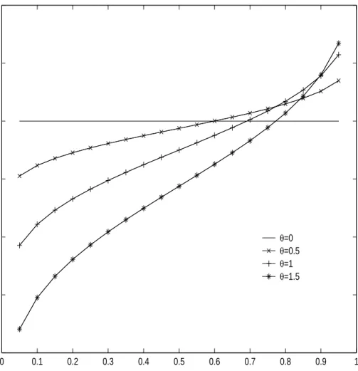
1 Plots of unpooled comparison density function of normal distri-butions with difference in locations assuming F = N(0,1) and G = N(θ,1). Unpooled comparison density is log d(u;F, G) = θΦ−1(u)− .5θ2 where Φ−1(u) is the inverse function of F = N(0,1). As the difference in locations is getting greater, compar-ison density is getting farther from log d(u) = 0(d(u) = 1). Also,
logd(u) is monotone. . . . . 9 2 Plots of unpooled comparison density function of normal
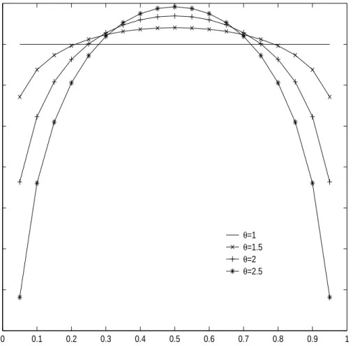
dis-tributions with difference in scales assuming F = N(0,1) and G= N(0, θ−2). Unpooled comparison density is log d(u;F, G) = logθ−.5 Φ−1(u)2(θ2−1) where Φ−1(u) is the inverse function of F = N(0,1). As the difference in scales is getting greater, com-parison density is getting farther from d(u) = 1(log d(u) = 0).
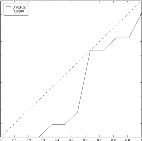
Also, log d(u) is quadratic and symmetric. . . . . 10 3 Plot of sample unpooled comparison distribution functionD∼(u;F, G)
with stress data. In this case, two properties of comparison dis-tribution function(D∼(0;G, F) = 0 and ,D∼(1;G, F) = 1) are not
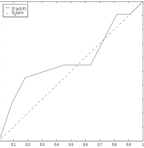
satisfied. . . . . 17 4 Plot of sample unpooled comparison distribution functionD∼(u;G, F)
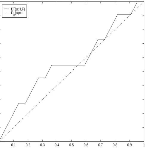
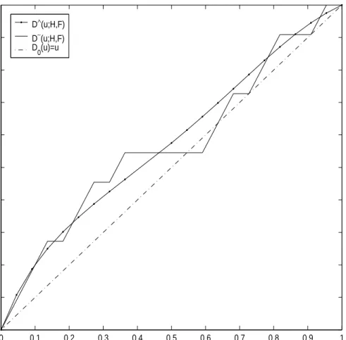
with stress data. . . . . 18 5 Plot of sample pooled comparison distribution functionD∼(u;H, F)
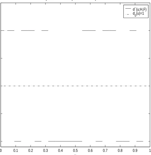
with stress data. . . . . 19 6 Plot of sample pooled comparison density function d∼(u;H, F)
with stress data. . . . . 20 7 Side by side boxplot with stress data. . . . . 21 8 Sample mid-distribution score functions up to order 4 using stress
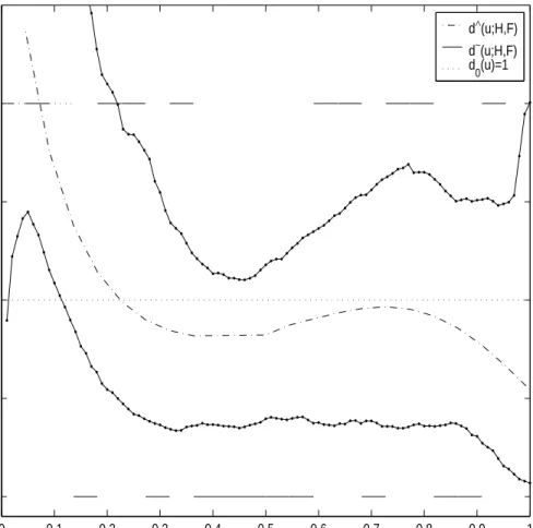
9 d∧(u;H, F) : Estimated comparison density function through ex-ponential model approach with stress data. The step function, the quartile density is added to the graph to see how exponen-tial model approach works. The quartile density is defined for i = 1,2,3,4 by dQk(u) = 4{D∼ i(.25)
− D∼ (i − 1)(.25)}, (i−1).25 < u < i(.25). For lower value of blood pressure(u < 0.25), the comparison density is greater than 1, indicating a great
frequency of observations in control group. . . . . 46 10 95% bootstrap confidence interval of d∧(u;H, F) : For better
in-terpretation, bootstrap confidence interval is added and the con-fidence interval is computed through percentile method with 500 bootstrap samples. Since the confidence interval does not include uniform density d0(u), we conclude that the distributions of the blood pressure level of two groups are different and stress does
have an effect on blood pressure level. . . . . 47 11 D∧(u;H, F) : Estimated comparison distribution function with
stress data. Since estimated comparison distribution function goes withD∼(u;H, F) very well, we conclude that our exponential
model estimation is working properly. . . . . 48 12 Sample pooled comparison distribution function with radon
can-cer data. . . . . 55 13 Sample mid-distribution score functions up to order 4 using radon
cancer data. ψj HN−1 u)) for ui−1 < u < ui and HN−1(ui) =zi. . . . . 56 14 d∼(u;H.F): Sample comparison density function with radon
can-cer data. . . . . 58 15 d∧(u;H, F) : Estimated comparison density function through
ex-ponential model approach with two components with radon cancer
data. . . . . 60 16 D∧(u;H, F) : Estimated comparison distribution function with
radon cancer data with 2 components. Since estimated compar-ison distribution function goes with D∼(u;H, F) very well, we conclude that our exponential model estimation is working
FIGURE Page 17 95% bootstrap confidence interval of d∧(u;H, F) : For better
in-terpretation, bootstrap confidence interval is added and the con-fidence interval is computed through percentile method with 500 bootstrap samples. Since the confidence interval does not include uniform density d0(u), we conclude that the distributions of the radon concentration level of two groups are different and radon
does have an effect on childhood cancer incidence. . . . . 62 18 Case 2: Same locations, scales but different distributions:
Proba-bility density functions ofX ∼N ormal(1,12) andY ∼Gamma(1,1). 68
19 Case 2: Same locations, scales but different distributions: d∧(u;H, F): Estimated comparison density function with X ∼N ormal(1,12) and Y ∼ Gamma(1,1). 2nd and 3rd order score functions were
selected(C ={2,3}). . . . . 69 20 Case 2: Same locations, scales but different distributions: D∧(u;H, F):
Estimated comparison distribution function withX ∼N ormal(1,12)
and Y ∼Gamma(1,1). . . . . 70 21 Case 3: Same locations, different scales and same distributions:
Probability density functions of X ∼ N ormal(0,52) and Y ∼
N ormal(0,12). . . . . 71 22 Case 3: Same locations, different scales and same distributions:
d∧(u;H, F): Estimated comparison density function with X ∼ N ormal(0,52) and Y ∼ N ormal(0,12). Only 2nd order score
function was selected(C ={2}). . . . . 72 23 Case 3: Same locations, different scales and same distributions:
D∧(u;H, F): Estimated comparison distribution function with
X ∼N ormal(0,52) and Y ∼N ormal(0,12) . . . . 73 24 Case 4: Different locations, but same scales and distributions:
Probability density functions of X ∼ N ormal(0,12) and Y ∼
25 Case 4: Different locations, but same scales and distributions: d∧(u;H, F): Estimated comparison density function with X ∼ N ormal(0,12) and Y ∼ N ormal(3,12). Only 1st order
compo-nent was selected(C ={1}). . . . . 75 26 Case 4: Different locations, but same scales and distributions:
D∧(u;H, F): Estimated comparison distribution function with
X ∼N ormal(0,12) and Y ∼N ormal(3,12) . . . . 76 27 Case 5: Same locations, but different scales and distributions:
Probability density functions of X ∼ N ormal(2,12) and Y ∼
Gamma(1,2). . . . . 77 28 Case 5: Same locations, but different scales and distributions:
d∧(u;H, F): Estimated comparison density function with X ∼ N ormal(2,12) and Y ∼ Gamma(1,2). 2nd, 3rd, and 4th order
score functions were selected(C ={2,3,4}). . . . . 78 29 Case 5: Same locations, but different scales and distributions:
D∧(u;H, F): Estimated comparison distribution function with
X ∼N ormal(0,12) and Y ∼N ormal(3,12) . . . . 79 30 Case 6: Different locations, same scales and different
distribu-tions: Probability density functions ofX ∼N ormal(0, √
22) and
Y ∼Gamma(1,2). . . . . 80 31 Case 6: Different locations, same scales and different
distribu-tions: d∧(u;H, F): Estimated comparison density function with X ∼ N ormal(0,
√
22) and Y ∼ Gamma(1,2). 1st and 2nd order
score functions were selected(C ={1,2}). . . . . 81 32 Case 6: Different locations, same scales and different
distribu-tions: D∧(u;H, F): Estimated comparison distribution function with X ∼N ormal(0,
√
22) and Y ∼Gamma(1,2) . . . . 82 33 Case 7: Different locations, scales but same distributions:
Proba-bility density functions ofX ∼N ormal(0,12) andY ∼N ormal(3,22). 83
FIGURE Page 34 Case 7: Different locations, scales but same distributions: d∧(u;H, F):
Estimated comparison density function with X ∼N ormal(0,12) and Y ∼ N ormal(3,22). 1st and 3rd order score functions were
selected(C ={1,3}). . . . . 84 35 Case 7: Different locations, scales but same distributions: D∧(u;H, F):
Estimated comparison distribution function withX ∼N ormal(0,12)
and Y ∼N ormal(3,22) . . . . 85 36 Case 8: Different locations, scales and distributions: Probability
density functions of X ∼N ormal(0,12) and Y ∼Gamma(2/3,2). . 86 37 Case 8: Different locations, scales and distributions: d∧(u;H, F):
Estimated comparison density function with X ∼N ormal(0,12) and Y ∼Gamma(2/3,2). 1st and 3rd order score functions were
selected(C ={1,3}). . . . . 87 38 Case 8: Different locations, scales and distributions: D∧(u;H, F):
Estimated comparison distribution function withX ∼N ormal(0,5)
CHAPTER I
INTRODUCTION
1.1. The Two-Sample Problem
Assume that we have a random sample X1,· · · , Xm from a continuous distribution F(y) =P(Xi ≤y), i= 1,· · · , m and a random sample Y1,· · · , Yn from a continuous distribution G(y) = P(Yi ≤ y), i = 1,· · · , n. Also assume independence of the two samples. The two-sample problem is about homogeneity of the two samples and formally can be stated as H0 : F = G. Even though we stated the two-sample problem in terms of distributions, the two-sample problem could be homogeneity in locations or in scales of the two samples. Borovkov (1998) provides several examples of the two-sample problem.
• A comparison of two processing techniques on the crops of some variety cereals. • A test of the effect of a new drug by means of comparing the state of patients
in two groups, one taking the drug and the other(the control group) not. • A comparison of the car accident ratios in two cities.
To solve the two-sample problem, a number of tests were proposed by statisticians in various contexts. Some of the tests need specific assumptions on the nature of two distributions. According to assumptions on distributions, we classify tests into The format and style of this dissertation follow that of Biometrics .
parametric test and nonparametric tests. Two typical tests are the two-sample t-test and the Wilcoxon’s rank sum test respectively. However, since they are testing the differences in locations, they do not extract more information from the data as well as a test of homogeneity of distribution functions. Even though the Kolmogorov-Smirnov test statistic or the Anderson-Darling test can be used for test of H0 : F = G, those statistics give no indication of the actual relation of F to G even though H0 : F = G is rejected. The point is why it was rejected. But most two-sample techniques can not answer this point. Our approach gives an answer using graphical tools which is a main property of our approach. Our approach is unified in the sense that graphs and tests are derived from a common foundation, comparison distribution and comparison density. The comparison density is graphical in nature and carries information regarding the relation of f tog.
The goal of this dissertation is to discuss the two-sample problem and our main contribution will be to implement and illustrate a two-sample data analysis proce-dure which extracts more information from the data by a methodology that makes almost no assumptions on two continuous distributions F and G. In that sense, our approach is nonparametric. Also, our approach gives graphical elements in the two-sample problem where typically exist not many graphical elements such as side by side boxplot, Q-Q plots and histograms which are not very informative. Also, our procedure will help researchers to make a conclusion to why two populations are dif-ferent when H0is rejected and to give an explanation to describe the relation between F and G in a graphical way.
1.2. Outline of This Dissertation
This dissertation is composed of six chapters and an appendix. Chapter I is an in-troduction of the two-sample problem. In Chapter II, concepts of comparison distri-bution function and comparison density function are discussed. Especially in section 2.3, sample versions of those functions are discussed for implementation in practice while population concepts are provided in section 2.2. Also, properties of comparison distribution and density functions are reviewed. In section 2.3, a real data set is used to illustrate sample concepts of those functions.
Chapter III examines exponential model with components with other necessary concepts such as mid-distribution functions, score functions and components. In sec-tion 3.2.4, we discuss exponential model approach to comparison density funcsec-tion. Maximum entropy interpretation of exponential model is also given in section 3.2.4.1. And the following section 3.2.4.2 is dedicated on estimation of coefficient of exponen-tial model.
Chapter IV provides an algorithm to solve the two-sample problem. That algo-rithm is based on comparison density estimation through exponential model approach. Chapter V applies the algorithm of Chapter IV to a real data set and to simulated data sets. Chapter VI presents conclusions and future research interests.
Appendix A gives some proofs of the theorems and properties stated in the previous chapters.
CHAPTER II
COMPARISON DISTRIBUTION FUNCTION AND COMPARISON DENSITY FUNCTION
2.1. Introduction
In this chapter, comparison distribution and comparison density functions are defined under the two-sample frame. As a graphical and functional type of test, Parzen (1983) introduced the concept of comparison density. In one-sample case, comparison distribution is comparing a model for a true distribution and the sample distribution. In the following sections, the comparison distribution and comparison density are defined and some properties of them are discussed.
2.2. Population Concepts
We can formulate the two-sample problem as the comparison of two continuous dis-tribution functions F and Gof variablesX and Y respectively. Assume that we have a sample X1,· · · , Xm from a continuous distribution F and a sampleY1,· · · , Yn from a continuous distribution G. Assume F and G have continuous densities f and g. LetN =m+n and λN =m/N. To compare two continuous distributions F and G, we define two versions of comparison distributions, unpooled comparison distribution D(u;F, G), and pooled comparison distribution function D(u;H, F) where 0≤u≤1 and H is defined by
assuming that limN→∞m/N = λ with 0 < λ < 1. Define the following inverse functions at 0≤u≤1:
F−1(u) = inf{y;F(y)≥u}, G−1(u) = inf{y;G(y)≥u},
H−1(u) = inf{y;H(y)≥u}. (2.2) The unpooled comparison distribution function is defined as
D(u;F, G) =G(F−1(u)), 0≤u≤1 (2.3) with assumptions that D(0;F, G) = 0 and D(1;F, G) = 1. The pooled comparison distribution function is
D(u) =D(u;H, F) =F(H−1(u)), 0≤u≤1. (2.4) Research on comparing the two distributions has tended to focus on estimating the unpooled estimator. However, if F and G do not have the same support, the com-parison distribution is not always rigorously definable. For example, suppose F is a distribution of incomes of men and G is a distribution of incomes of women. Then, the support of F may not be contained in that of G. Therefore, Parzen (1997) rec-ommends to use the pooled comparison distribution. The properties of D(u) are as follows:
• D(0) = 0. • D(1) = 1.
• D(u) is non-decreasing on [0,1]. • D(u) is absolutely continuous on [0,1]
Another problem of the unpooled comparison distribution is that the first two properties (D(0) = 0 and D(1) = 1) may not be satisfied with the sample unpooled comparison distribution which will be defined in the section 2.3. We will explain this in detail with an example in the section 2.3.
Derivatives of D(u) are called the comparison density functions. The unpooled comparison density function d(u;F, G) and the pooled comparison density function d(u;H, F) are defined respectively by
d(u;F, G) = D0(u;F, G) = g(F −1 (u)) f(F−1(u)), d(u;H, F) = D0(u;H, F) = f(H −1(u)) h(H−1(u)) = f(H −1(u)) λf(H−1(u)) + (1−λ)g(H−1(u)). (2.5) We requiref(x) = 0 impliesg(x) = 0 in order for d(u;F, G) to be well defined and to integrate to 1. Given a plot ofd(u), one can interpret the various shapes as indicating that the difference between two distributions(F and G for unpooled case andH and F for pooled case) is a difference in location or a difference in scale by the following known theorem.
Theorem 2.1. (Parzen (1998)) Assume F =N(θ0,1) and G=N(θ,1); that is, the
difference between two Normal distributions is due to a difference in location. Then, the unpooled comparison density satisfies
log d(u;F, G) = (θ−θ0)Φ−1(u)−.5(θ−θ0)2. (2.6) where F = Φ which is the standard normal distribution. When F = N(0, θ0−2) and G=N(0, θ−2), that is, if there is a difference in scale, unpooled comparison density satisfies
log d(u;F, G) = log θ
θ0 −.5 Φ −1
Proof d(u;F, G) = g F −1(u) f F−1(u) = 1 √ 2π exp −(Φ−1(u)−θ)2 2 1 √ 2πexp −(Φ−1(u)−θ0)2 2
⇒ log d(u;F, G) = (θ−θ0)Φ−1(u)−.5(θ2−θ20). (2.8)
d(u;F, G) = g F −1 (u) f F−1(u) = θ √ 2πexp −θ2Φ−1(u)2 2 θ0 √ 2πexp −θ02Φ−1(u)2 2
⇒ log d(u;θ) = log θ
θ0 −.5(Φ −1
(u))2(θ2−θ02). (2.9) For pooled comparison density with difference in locations, assume F =N(0,1) and G = N(θ,1). Then for a given λ, pooled distribution H(y) is a mixture normal distribution.
H(y) =λN(0,1) + (1−λ)N(θ,1).
For pooled comparison density with difference in scales, assume F = N(0,1) and G = N(0, θ−2). Then for a given λ, pooled distribution H(y) is a mixture normal distribution.
H(y) = λN(0,1) + (1−λ)N(0, θ−2).
In the case of pooled comparison density, we do not have a closed form like unpooled comparison density functions. Thus, pooled comparison density can be computed by simulations. In simulation, a very large sample of random variables from known
distributions F(y) and G(y) will be generated. Then, sample pooled comparison distribution and density function can be computed.
For the unpooled case, Figure 1 and Figure 2 present log d(u;F, G) for a vari-ety of F and G. If two distributions F and G are homogeneous, d(u;F, G) = 1(or log d(u;F, G) = 0). As the difference in locations is getting greater, comparison den-sity is getting farther fromd(u;F, G) = 1( or log d(u;F, G) = 0). Also, log d(u;F, G) is monotone for location difference and quadratic for scale difference. As the difference in scales is getting greater, comparison density is getting farther from d(u;F, G) = 1(or log d(u;F, G) = 0). Also, log d(u;F, G) is quadratic and symmetric since there is no difference in location.
Parzen (1983) gives some properties of pooled comparison densityd(u) =d(u;H, F). • 0≤d(u)≤1/λ
• d(u)→0 if f →0 • d(u)→1/λ if g →0
For the proofs, see appendix A. From the definition of the pooled comparison density function, we can see the relationship between d(u) and likelihood ratio(g/f). Parzen (1983) noted that
1
d(u) =λ+ (1−λ)
g(H−1(u))
f(H−1(u)) (2.10)
which is derived from equation(2.5). If an estimate of g/f is not really desired, it is enough to know that d(u) > 1 if and only if g(H−1(u)) > f(H−1(u)). Also, even thoughg/f is not bounded,d(u) is bounded between 0 and 1/λ. Since the estimation
0 0.1 0.2 0.3 0.4 0.5 0.6 0.7 0.8 0.9 1 −4 −3 −2 −1 0 1 2 log d(u;F,G) u θ=0 θ=0.5 θ=1 θ=1.5
Figure 1. Plots of unpooled comparison density function of normal distributions with difference in locations assumingF =N(0,1) andG=N(θ,1). Unpooled comparison density is log d(u;F, G) = θΦ−1(u)−.5θ2 where Φ−1(u) is the inverse function of
F =N(0,1). As the difference in locations is getting greater, comparison density is getting farther from log d(u) = 0(d(u) = 1). Also, log d(u) is monotone.
0 0.1 0.2 0.3 0.4 0.5 0.6 0.7 0.8 0.9 1 −7 −6 −5 −4 −3 −2 −1 0 1
Comparison Density Plot with Scale Difference
log d(u;F,G) u θ=1 θ=1.5 θ=2 θ=2.5
Figure 2. Plots of unpooled comparison density function of normal distributions with difference in scales assuming F =N(0,1) and G=N(0, θ−2). Unpooled comparison density is log d(u;F, G) = log θ −.5 Φ−1(u)2(θ2 −1) where Φ−1(u) is the inverse function of F = N(0,1). As the difference in scales is getting greater, comparison density is getting farther from d(u) = 1(log d(u) = 0). Also, log d(u) is quadratic and symmetric.
of unbounded functions is more difficult, we recommend to use pooled comparison density function d(u) for estimation of a likelihood ratio.
Comparison distribution and comparison density concepts can be used to compare two discrete distributionsF and Gwith respective probability mass functionspF and pG. We define a comparison density function
d(u) =d(u;F, G) =pG(F−1(u))/pF(F−1(u)); (2.11) then define a unpooled comparison distribution function
D(u) =D(u;F, G) =
Z u 0
d(t)dt (2.12)
assuming pF(x) = 0 implies pG(x) = 0. D(u;F, G) is piecewise linear between its values at uj =F(xj), where x1 <· · ·< xm and D(uj;F, G) = G(F−1(uj)) = G(xj).
Pooled comparison distribution and comparison density functions are defined as d(u) = d(u;H, F) =pF(H−1(u))/pH(H−1(u)),
D(u) = D(u;H, F) =
Z u 0
d(t)dt. (2.13)
assuming pF(x) = 0 implies pH(x) = 0. D(u;H, F) is piecewise linear between its values at uj =H(zj), where z1 <· · ·< zN and D(uj;H, F) =F(H−1(uj)) =F(zj).
The graph of a comparison distribution D(u;F, G) or D(u;H, F) is called a P-P plot because it is a plot of F(y), G(y) or H(y), F(y) which compares the p values of an observation y under the two distributions. A P-P plot can be drawn by linearly connecting the points (0,0), (1,1), F(y), G(y) or H(y), F(y) for F -exact uj =F(yj)(j = 1,· · · , m) or H-exact uj = H(yj)(j = 1,· · · , N) respectively. And this is equal to the definition of D(u) in discrete case. By using P-P plot, we
have a continuous sample distribution and can overcome the problem that sample distributions are discrete. P-P plot can be used as an analysis tool and provide the basis of further analysis.
2.3. Sample Comparison Distribution and Comparison Density Functions
For theoretical concepts to be applied to data analysis, it is crucial to define sam-ple version of those concepts. Assume that we have a samsam-ple X1,· · · , Xm from a continuous distribution F and a sample Y1,· · · , Yn from a continuous distribution G. Let Z1,· · ·, ZN be a pooled sample ofX1,· · · , Xm andY1,· · · , Yn. Assume F and G have continuous densities f and g. Let N =m+n and λN =m/N. Define sample distribution functions Fm(x) = m X t=1 I(Xt ≤x)/m Gn(y) = n X t=1 I(Yt ≤y)/n HN(z) = λNFm(z) + (1−λN)Gn(z), x, y, z ∈R (2.14) where I(Y ≤ y) = 1 if Y ≤ y and I(Y ≤ y) = 0 otherwise. HN is a sample pooled distribution ofFm andGn. The sample pooled distributionHN =λNFm+ (1−λN)Gn is equivalent to computing HN(y) =
Pm
t=1I(Xt ≤y)/N +
Pn
t=1I(Yt ≤y)/N.
Example: For illustration of concepts in this section on interesting data, we use a dataset from Giampaoli and Singer (2004) and call it as stress data. They consider the problem of comparing the mean of diastolic blood pressure of two group of individuals. One group is exposed to a stress stimulus (like the death of a close relative or discharge from employment) and another group is under normal conditions. The data are reproduced in Table 1 and each data value corresponds to the average of series of 30 measurements taken over periods of one hour to eliminate short term
Table 1
Diastolic blood pressure (mmHg)
Stress group Control group
87.1 81.5 89.6 81.7 92.2 85.5 92.2 88.9 92.2 89.4 92.4 89.9 92.7 93.5 95.0 94.6 96.4 95.4 96.8 95.5 109.2 97.0
fluctuations. In this data, there are ties which means one value occurs several times like 92.2 in stress group. We consider F as distribution function of control group and G as distribution function of stress group. With this stress data, we compute sample distribution functions(Table 2- Table 4) using equaiton (2.14). Now we have X1,· · · , X11(m= 11) for control group, and Y1,· · · , Y11(n = 11) for stress group and thus N =m+n= 22. Thus λ =m/N = 11/22 = 1/2.
The sample unpooled comparison distribution is defined as a continuous function ofu by
D∼(u;F, G) = Gn(Fm−1(u)) (2.15) atuequal toF-exact valueuj(j = 1,· · · , m) satisfyingFm(xj) =ujfor distinctxj val-ues(Table 2). At other values of u, defineD∼(u;F, G) by linear interpolation between its values at F-exact values of uj. Figure 3 and 4 are the plots of sample unpooled comparison distribution. Sample unpooled comparison distribution functions are de-fined by D∼(u;F = Control, G = Stress) and D∼(u;G = Stress, F = Control)
Table 2
Sample distribution function for control group : Fm(x) =P m t=1I(Xt ≤x)/m, m = 11 Blood pressure Fm 81.5 0.0909 81.7 0.1818 85.5 0.2727 88.9 0.3636 89.4 0.4545 89.9 0.5455 93.5 0.6364 94.6 0.7273 95.4 0.8182 95.5 0.9091 97.0 1.0000 Table 3
Sample distribution function for stress group : Gn(y) =
Pn
t=1I(Yt ≤y)/n, n = 11. The number in() means the number of occurrences of the corresponding observation.
Blood pressure Gn 87.1 0.0909 89.6 0.1818 92.2(3) 0.4545 92.4 0.5455 92.7 0.6364 95.0 0.7273 96.4 0.8182 96.8 0.9091 109.2 1.0000
Table 4
Sample pooled distribution function HN(z) =
Pm t=1I(Xt ≤z)/N +Pnt=1I(Yt ≤z)/N, N = 22 Blood pressure HN 81.5 0.0455 81.7 0.0909 85.5 0.1364 87.1 0.1818 88.9 0.2273 89.4 0.2727 89.6 0.3182 89.9 0.3636 92.2(3) 0.5000 92.4 0.5455 92.7 0.5909 93.5 0.6364 94.6 0.6818 95.0 0.7273 95.4 0.7727 95.5 0.8182 96.4 0.8636 96.8 0.9091 97.0 0.9545 109.2 1.0000
respectively for each figure. Specially from Figure 3, we can know that property of comparison distribution(D(1) = 1) mentioned in section 2.2 is not satisfied. Sample pooled comparison distribution is
D∼(u;H, F) = Fm(HN−1(u)) (2.16) at H-exact values uj(j = 1,· · ·, r) satisfying HN(zj) = uj for distinct zj values( Table 4) and at other values of u by linear interpolation between its values at H-exact values of u. Figure 5 is a plot of the sample pooled comparison distribution function with stress data. From sample comparison distribution, we compute the
sample comparison density d∼(u) which is used as an estimate ofd(u). Actually, the slope of the sample comparison distribution is the sample comparison density. For the unpooled case,
d∼(u;F, G) = D ∼(u
j;F, G)−D∼(uj−1;F, G) uj −uj−1
if uj−1 < u < uj (2.17) where u0 = 0, and uj =Fm(xj),(j = 1,· · ·, m). For the pooled case,
d∼(u;H, F) = D ∼
(uj;H, F)−D∼(uj−1;H, F) uj −uj−1
if uj−1 < u < uj (2.18) where u0 = 0, and uj = HN(zj) for j = 1,· · · , N). Since our main concern is the pooled comparison density function, we have only a plot of the sample pooled comparison density function. See Figure 6. A pattern in a sample comparison density function indicates direction of shape of the score function whose statistic will be significant and therefore we could conclude a proper model for the difference of the two distributions. From Figure 6, we can see a quadratic pattern or somewhat cubic pattern and this may indicate the difference in the direction of 2nd(scale diffeence) or 3rd order score function. From the side by side boxplot of Figure 7, we see some differences in scale between two groups. In the Chapter III, we will have a more precise conclusion using the exponential model approach to the two-sample problem.
0 0.1 0.2 0.3 0.4 0.5 0.6 0.7 0.8 0.9 1 0 0.1 0.2 0.3 0.4 0.5 0.6 0.7 0.8 0.9 1
Sample Unpooled P−P Plot of D(u;F,G)
D ∼ (u;F,G) u D∼(u;F,G) D 0(u)=u
Figure 3. Plot of sample unpooled comparison distribution function D∼(u;F, G)
with stress data. In this case, two properties of comparison distribution function(D∼(0;G, F) = 0 and ,D∼(1;G, F) = 1) are not satisfied.
0 0.1 0.2 0.3 0.4 0.5 0.6 0.7 0.8 0.9 1 0 0.1 0.2 0.3 0.4 0.5 0.6 0.7 0.8 0.9 1
Sample Unpooled P−P Plot of D(u;G,F)
D ∼ (u;G,F) u D∼(u;G,F) D 0(u)=u
Figure 4. Plot of sample unpooled comparison distribution function D∼(u;G, F)
0 0.1 0.2 0.3 0.4 0.5 0.6 0.7 0.8 0.9 1 0 0.1 0.2 0.3 0.4 0.5 0.6 0.7 0.8 0.9 1
Sample Pooled P−P Plot of D(u;H,F)
D ∼ (u;H,F) u D∼(u;H,F) D 0(u)=u
Figure 5. Plot of sample pooled comparison distribution functionD∼(u;H, F) with
0 0.1 0.2 0.3 0.4 0.5 0.6 0.7 0.8 0.9 1 0 0.5 1 1.5 2 2.5
Sample Pooled Comparison Density Function
d ∼ (u;H,F) u d∼(u;H,F) d 0(u)=1
Figure 6. Plot of sample pooled comparison density functiond∼(u;H, F) with stress
1=Control 2=Stress 85 90 95 100 105 110
Side by Side Boxplot
Blood Pressure
CHAPTER III
EXPONENTIAL MODEL WITH COMPONENTS
3.1. Introduction
In this chapter, we introduce an exponential model approach to the comparison den-sity estimation and related concepts. To form an exponential model, we need to design mid-distribution score functions first. In subsection 3.2.1, we define the concept of mid-distribution function introduced by Parzen (1989) and in subsection 3.2.2, we provide a definition and recursive formula of mid-distribution score functions with an example.
To estimate the comparison density function, the exponential model with com-ponents will be used. For the estimation of comparison density d(u), there have been two main approaches. One is kernel density estimation and another is autore-gressive method. For details of each method, see Woodfield (1982) and Carmichael (1976) respectively. Our exponential model approach is similar to exponential family based density estimation, orthogonal series density estimation and maximum entropy method. Exponential family based density estimation is approximating a density function by using a member of a family of densities. Consider an exponential family of densities of the form
d(u;θ) = exp K X k=1 θkφk(u)−ΨK(θ) , 0< u <1 (3.1) where θ = (θ1,· · · , θK) ∈ Θ = {θ ∈ RK : K(θ) <∞}. The function ΨK(θ) is the
normalizing value so that each density integrates to one: ΨK(θ) = log (Z 1 0 exp K X k=1 θkφk(u) du ) (3.2) and {φk(u)}Kk=1 are basis functions, which are bounded and linear independent func-tions such that
SK =span{1,{φk(u)}Kk=1}
is a linear space. Three common choices for the basis functions are polynomials, trigonometric series, and spline bases. However disadvantage of this approach is the assumption that the comparison density is actually a member of this family which we do not assume in our exponential model approach.
Orthogonal series density estimation was introduced by Cencov (1962) and is al-lied with exponential family estimation. Cencov (1962) considers the expansion using orthogonal system with respect to a weight function. Basically Cencov’s approach is a method of moments estimating scheme(Woodfield (1982)). Other researchers exam-ined Cencov’s method using specific system of orthogonal functions. Schwartz (1967) considers expansions using Hermite polynomials, Tarter and Kronmal (1970)) con-sider trigonometric systems(Fourier series expansion), and Crain (1974) uses Legendre polynomials. Consider the orthogonal series family of functions:
d(u;θ) =θ0+ ∞ X
k=1
θkφk(u), 0< u <1 (3.3) whereθk ∈ R and {φk(u)}∞k=1 form a complete orthonormal basis for the space of all square integrable functions on [0,1]. Orthonormal means that
Z 1
0
φi(u)φj(u)du=I(i=j)
sequence of constants {θk}Kk=1 such that |d(u)− K X k=1 θkφk(u)|2 →0 asK → ∞. Thus, one can write
d(u) =θ0+ ∞ X k=1 θkφk(u), 0< u <1 so that θk = Z 1 0 φk(u)d(u)du=E φk(u) . In practice, the comparison density might be estimated by
d∧(u;θ) =θ0∧+ K
X
k=1
θk∧φk(u), 0< u <1.
for suitable choice of order K and θ∧k =Pmj=1φk(Rj)/m where Rj is the rank of the sample in the pooled sample. Note that the estimator has the undesirable property that it may be negative for some value of u while our exponential model approach guarantees the nonnegativity of the estimate.
3.2. Basic Concepts
3.2.1. Mid-distribution Functions
Ranks of the observations are one of the important elements of nonparametric sta-tistics. Parzen (1989) presented a concept of the mid-distribution function which is a transform of ranks. To compute distribution score functions, we define mid-distribution functions first. Let F be a discrete distribution function. For distinct x values,
whereF(x) =P[X ≤x] andpF(x) =P[X =x]. For order statisticsX(1;m)≤ · · · ≤ X(m;m) of a sample X1,· · · , Xm with no ties,
Fmid(X(j;m)) = (j−.5)
m =
Rj −.5
m (3.5)
which transforms the rank Rj to a number in the open unit interval, and is called mid-rank transform. If any X values are tied, their average rank is used for Rj. IfX is a continuous random variable, Fmid(X) ∼ U nif orm(0,1). This mid-distribution concept is important for discrete distributions, specially for sample distribution func-tions since sample distribution funcfunc-tions are discrete even though true distribution functions are continuous. For the mid-distribution transform W =Fmid(X),
µmid = E W = 0.5 σmid2 = V AR W = [1−E p2F(X) ]/12. (3.6)
For equations in (3.6), there have been a few proofs and Parzen (2004) provides outline of a simple proof. For the proof of equations in (3.6), we adopt Parzen’s approach. For detail, see appendix A.
In practice, assume that we have a sampleX1,· · · , Xm. Then we estimateFmid(x) from Fmmid(x) =Fm(x)−.5p∼F(x) (3.7) where Fm(x) = Pm i=1I(X ≤ x)/m and p ∼
F(x) = 1/m with no ties. If there are ties, p∼F(x) =
Pm
t=1I(Xt =x)/m. Specially in the two-sample frame, let Z1,· · ·, ZN be a pooled sample with a sample distribution function HN(z). Then, sample mid-distribution can be computed by
where Hmid N (z) =
PN
t=1I(Zt ≤ z)/N and p∼H(z) =
PN
t=1I(Zt = z)/N. With stress data, we compute HN(z),p∼H(z), and H
mid
N (z) in Table 5. 3.2.2. Design of Score Functions
LetX be a variable with distribution functionF. Then a score function ψ is defined satisfying
E ψ(X) = 0,
V AR ψ(X) = 1 (3.9)
where expectation is taken with respect to a specific distribution ofX. For discrete F, we define orthonormal score functions which are based on ranks through mid-distribution transform. By Gram-Schmidt orthonormalization, we derive orthogo-nal polynomials, called mid-distribution score functions, recursively. Define w1(X), φ1(X) and ψ1(X). w1(X) = Fmid(X)−µmid, φ1(X) = w1(X), ψ1(X) = p φ1(X) hφ1(X), φ1(X)i = Fmid(X)−µmid σmid (3.10) where h·,·i is inner product of two functions, µmid =E Fmid(X)
= 0.5 and σmid2 = V AR Fmid(X) which are defined in the previous subsection 3.2.1. For j = 2,3,· · ·, we have a recursive form
wj(X) = ψ j 1(X)−βj, φj(X) = wj(X)− j−1 X i=1 hφj(X), ψi(X)iψi(X), ψj(X) = φj(X) p hφj(X), φj(X)i (3.11)
where βr =E[ (F (X)−0.5)/σmid ]. A few terms of mid-distribution score func-tions ψj(X) are derived as follows;
ψ0(X) = 1 ψ1(X) = (Fmid(X)−.5)/σmid ψ2(X) = (ψ12(X)−1)−β3ψ1(X)/a2 .. . (3.12) where a2 2 = β4 −β 2
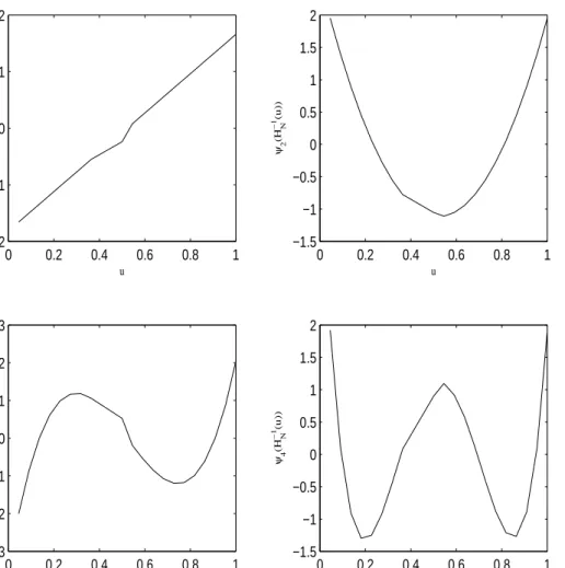
3 −1. Also, the equations in (3.9) are satisfied by the orthonor-mality of ψ functions. In the two-sample work in practice, let Z1, Z2,· · · , ZN be a pooled sample with a sample distribution HN(z). Then, the sample mid-distribution is computed by equation (3.8). With the stress data, we compute mid-distribution score functions up to order 4 by using the above recursive formula in equation(3.11). Figure 8 shows a plot of each sample mid-distribution score function. The plots are on the unit interval and plottingψj H
−1
N u)) forui−1< u < ui and H −1
N (ui) = zi. Prac-tically we can verify the orthornormality of sample mid-distribution score functions defined on the unit interval using stress data. See the Table 6.
3.2.3. Components
The usefulness ofd(u;H, F) comparingF andHarises from the fact thatd(u;H, F) = 1 iff H(y) = F(y). Thus one method to compare F and H can be based on a comparison of d(u;H, F) with the uniform density p0(u) = 1 when 0 ≤ u ≤ 1. Eubank et al. (1987) gives the introduction of a measure of the disparity between d(u;H, F) andp0(u) and analysis of its component decomposition. Define the measure using the squared L2[0,1] norm of their differences
φ2 =kd−p0 k2=
Z 1
0
Let {ψi H−1(u)
}∞
i=1 be an orthonormal system for L2[0,1] such that d−p0 ∼ ∞ X j=1 θjψj H−1(u) (3.14) where theθj’s are generalized Fourier coefficients.
θj = Z 1 0 (d(u)−1)ψj H−1(u) du= Z 1 0 d(u)ψj H−1(u) du, j = 1,2,· · · (3.15) and ∼ is the usual Fourier series notation indicating Prj=1θjψj →d−p0 in L2[0,1] as r→ ∞. By Parseval’s relation, φ2 = ∞ X j=1 θ2j (3.16)
where θj’s are components of φ2. Thus, to test H0 : F = H is equivalent to test H0 :φ2 = 0 or to testθ
j = 0 for allj ≥1 from equation (3.16). Since one cannot test an infinite number of parameters, Eubank et al. (1987) suggest to test subhypotheses, such asH0 :θj = 0 forj = 1,· · · , M for a constantM. H0 :F =Hshould be rejected if we can reject any of the subhypotheses θj = 0(j = 1,· · · , M). To estimate θj, make the change of variable x=H−1(u) in equation(3.15). Then,
θj = Z 1 0 d(u)ψj H−1(u) du = Z 1 0 f H−1(u) h H−1(u)ψj H −1 (u)du = Z ∞ −∞ f(x) h(x)ψj(x)h(x)dx = Z ∞ −∞ ψj(x)f(x)dx = Ef(ψj(x)) (3.17)
Thus, given estimates Fm and HN for F and H, the estimate of θj is θj∼ = Z ∞ −∞ ψj(x)dFm(x) = m∗ X i=1 p∼F(x ∗ i)ψj(x∗i) = EF(ψj(x)) (3.18)
where x∗i is the distinct value of the first sample Xi in the pooled sample ofX andY and m∗ is the number of distinct values in the sample ofX andp∼
F(x ∗ i) = Pm∗ i=1I(X = x∗
i)/m. To testH0 :θj = 0, we need to know asymptotic distribution of the individual components. For that, the corollary of Eubank et al. (1987) is used, which is a variant of the Chernoff-Savage theorem(Chernoff and Savage (1958)). Chernoff and Savage (1958) define a rank statistic having the form
SN = Z ∞ −∞ JN HN(x) dFm = 1 m m X j=1 JN(Ri/N) (3.19)
where Ri is the rank of Xi in the pooled sample, JN is known as a score function, and Fm and HN are sample distributions defined in Chapter II. Using the following Chernoff-Savage approach, we demonstrate normality of θ∼
j .
Theorem 3.1.(Chernoff and Savage, 1958). If J(u) is not constant and if |J(i)| ≤ K|u(1−u)|−i−(1/2)+δ for i = 0,1,2 and some K and δ > 0, then for fixed and con-tinuous F and G, one has SN is AN(µ, σN2 ), where
µ=
Z
and
N σ2N = 2(1−λN){
ZZ
x<y
G(x) 1−G(y)J0 H(x)J0 H(y)dF(x)dF(y) + 1−λN
λN
ZZ
x<y
F(x) 1−F(y)J0 H(x)J0 H(y)dG(x)dG(y)} (3.21) providing σN 6= 0.
The notationSN isAN(µ, σN2) means that the distribution function of the random variable (SN−mu)/σN converges pointwise to the distribution function of a standard normal random variable. To find approximate values of the distribution function of SN, one need only calculate the values of µandσN2 . In many practical circumstances, the values of µand σ2
N can be worked out. For an example, see Alexander (1989). θ∼
j ’s asymptotic distribution under the null hypothesis F = G or θj = 0, j = 1,2,· · · is given in the following theorem.
Theorem3.2. Under H0 :θj = 0, the asymptotic distribution of
√ N θ∼j is N(0, σ 2 j) where σj2 = 1−λ λ Z 1 0 ψj2(H−1(u))du= 1−λ λ . For the proof, see Alexander (1989). And σ2
j is estimated by σj∼2 =
1−λN λN
.
Then we find significant components by testing H0 : θj = 0, j = 1,· · · , M through standardization. Since we know the asymptotic distribution ofθ∼
j which is an estimate of θj from Theorem 3.2, if the result of standardization is greater than 2(or 3) in absolute value, we conclude that θj is not zero or significant(or very significant). With stress data, we have θ∼
values defined as Cj = N(θj )/σj θ1∼ =−0.2367 σ ∼ 1 = 1 θ2∼ = 0.2456 σ2∼= 1 θ3∼ =−0.2591 σ3∼= 1 θ4∼ =−0.2088 σ ∼ 4 = 1 then, C1 = −1.1102, C2 = 1.1520, C3 = −1.1253, C4 = −0.9794.
Thus, one may be able to conclude that there are no significant components through the test results. Therefore there is not enough evidence to reject H0 : θj = 0 for j = 1,2,3,4. This could mean thatd(u;H, F) is not different fromp0(u) = 1 and we could conclude that there is no significant evidence to reject H0 :F =G.
3.2.4. Exponential Model Approach and Comparison Density Estimation
The model discussed in this dissertation is motivated by the observation that the logarithm of a probability function is often found to be a fairly well-behaved func-tion and it is often convenient to work with it. In terms of density estimafunc-tion, the exponential model guarantees the nonnegativity of the density function which is an essential property of a density function.
Our exponential model is formed using score functions which have largest compo-nents instead of finding significant compocompo-nents through tests performed in the
previ-ous subsection 3.2.3. With selected components and corresponding mid-distribution score functions, we form an exponential model estimator of comparison density func-tion: d∧(u;θ) = exp θ∧0 + X k∈C θk∧ψk H−1(u) (3.22) where C is a set of index of selected components. With stress data, we sortθ∼
j values in absolute value in descending order.
θ∼3 = −0.2591 θ∼2 = 0.2456 θ∼1 = −0.2367 θ∼4 = −0.2088
Then with the three two components, an exponential model estimator of is d∧(u;θ) = exp θ∧0 +X
C
θk∧ψk H−1(u)
(3.23) where C ={1,2,3}. Estimation ofθk∧ will be discussed in 3.2.4.2.
3.2.4.1. Maximum Entropy Interpretation of Exponential Model Approach
Our comparison density estimator using exponential model approach has a maximum entropy interpretation in the sense that maximum entropy density estimation gives the same form of estimator as exponential model estimator. However, our exponen-tial model is different in the sense that we use orthonormal score functions as basis functions and use significant terms.
Shannon’s measure of entropy was originally developed for a discrete distribution. The entropy of a discrete distribution, denoted by HS(·) is defined
HS(p) =−
X
x
p(x) log p(x) (3.24)
where p(x) is probability mass function. The notion of entropy for a continuous distribution is formally defined by
HS(f) =−
Z ∞
−∞
f(y) log f(y)dy (3.25)
with probability density functionf(y). Another fundamental concept is cross-entropy defined by
H(f;g) =
Z ∞
−∞
−logg(y)f(y)dy (3.26) A closely related concept is Kullback-Leibler’s information divergence I(f;g) between two probability density functionsf(y) andg(y). The information divergence is defined by I(f :g) = Z ∞ −∞ −log g(y) f(y) f(y)dy. (3.27)
Then one important property of I(f;g) is
I(f;g)≥0 (3.28)
0 0.2 0.4 0.6 0.8 1 −2 −1 0 1 2 ψ1 (H N −1 (u)) u 0 0.2 0.4 0.6 0.8 1 −1.5 −1 −0.5 0 0.5 1 1.5 2 ψ2 (H N −1 (u)) u 0 0.2 0.4 0.6 0.8 1 −3 −2 −1 0 1 2 3 ψ3 (H N −1 (u)) u 0 0.2 0.4 0.6 0.8 1 −1.5 −1 −0.5 0 0.5 1 1.5 2 ψ4 (H N −1 (u)) u
Figure 8. Sample mid-distribution score functions up to order 4 using stress data. ψj HN−1 u)) for ui−1 < u < ui and HN−1(ui) =zi.
Exponential model for comparison density d(u;H, F) has a form log d(u;H, F) = K X j=1 θjψj H−1(u) −Ψ0(θ) (3.29) where Ψ0(θ) = log Z 1 0 ePKj=1θjψj H−1(u) du (3.30) and θ= (θ1,· · · , θK).
Theorem 3.3. Among any comparison density d(u) satisfying the following
con-straints Z 1 0 ψj H−1(u) d(u)du=τj, j = 1,· · · , M, an exponential model d0(u) has maximum entropy.
proof: I d(u);d0(u) = Z 1 0 −log d0(u) d(u) d(u)du = Z 1 0
−log d0(u)d(u)du+
Z 1
0
log d(u)d(u)du = HS d(u);d0(u) −HS d(u) (3.31) H(d(u);d0(u)) = Z 1 0
−log d0(u)d(u)du = Z " − M X j=1 θjψj H−1(u) −Ψ0(θ) # d(u)du = −Ψ0(θ)− M X j=1 θjτj = HS d0(u) (3.32)
Thus,
I d0(u);d(u) = HS d(u);d0(u)
−HS d0(u) ≥0 by equation(3.28) ⇒ HS d0(u) ≥HS d(u) (3.33) Therefore, an exponential model of comparison density function d(u) has maximum entropy.
3.2.4.2. Estimation of Coefficients of An Exponential Model
To estimate coefficients ofd∧(u) of equation (3.22), we adopt the method of moments. The method of moments is a technique for constructing estimators that is based on matching the sample moments with the corresponding distribution moments. Let
µ∼k(θ) = Z 1 0 d∼(u)ψk H−1(u) du (3.34)
denote the kth sample moment where k= 1,2,· · ·, K. Next, let µk(θ) = Z 1 0 d∧(u)ψk H−1(u) du (3.35)
denote the kth moment. To construct estimators of coefficients of exponential model, we need to solve the set of simultaneous equations
µ∼1(θ) = µ1(θ), µ∼2(θ) = µ2(θ),
.. .
Then equations in (3.36) can be rewritten by Mk(θ) =
Z 1
0
d∧(u)−d∼(u)ψk H−1(u)
du= 0, k = 1,2,· · · , K, (3.37) whereθ= (θ1,· · · , θK)0 and those satisfying constraints Mk(θ) = 0 have a maximum entropy interpretation from theorem 3.3. Assume we have 4 components θk, k = 1,2,3,4. Then the solutions are updated according to the scheme from Newton-Raphson method
θ(i+1) =θ(i)+ ∆θi,
where iindicates the iteration number and ∆θ= (∆θ1,∆θ2,∆θ3,∆θ4)0. We have the Jacobian system with starting values θk(0),k = 1,2,3,4.
∂M1(θ) ∂θ1 ∂M1(θ) ∂θ2 ∂M1(θ) ∂θ3 ∂M1(θ) ∂θ4 ∂M2(θ) ∂θ1 ∂M2(θ) ∂θ2 ∂M2(θ) ∂θ3 ∂M2(θ) ∂θ4 ∂M3(θ) ∂θ1 ∂M3(θ) ∂θ2 ∂M3(θ) ∂θ3 ∂M3(θ) ∂θ4 ∂M4(θ) ∂θ1 ∂M4(θ) ∂θ2 ∂M4(θ) ∂θ3 ∂M4(θ) ∂θ4 ∆θ1 ∆θ2 ∆θ3 ∆θ4 =− M1(θ) M2(θ) M3(θ) M4(θ)
which is obtained by Taylor expansion with ∂Mk(θ) ∂θl = Z 1 0 exp " θ0 + 4 X j=1 θjψj H−1(u) # ψk H−1(u) ψl H−1(u) du. (3.38) In practice, initial values are computed from
θk(0) = m∗
X
i=1
p∼F(x∗i)ψj(x∗i) k = 1,2,3,4 (3.39) which is from equation (3.18). Table 7 provides the result of Newton-Raphson it-eration to estimate the components of exponential model using stress data. Three components was chosen from subsection 3.2.4. Then, the estimated exponential model
is
d∧(u;θ) = exp −0.052−0.2171ψ1 H−1(u)+0.0922ψ2 H−1(u)−0.1862ψ3 H−1(u). (3.40) From the estimated coefficients, we could know that two distributions may be different in the direction of 1st and 3rd score functions.
To check the goodness of fit of our exponential model, we compute a smooth comparison distribution function and this wil be discussed in Chapter IV.
Table 5
Sample mid-distribution function Hmid
N (z) : H mid N (z) =HN(z)−.5p∼H(z) Blood pressure Rj HN p∼H(z) H mid N (z) 81.5 1 0.0455 0.0455 0.0227 81.7 2 0.0909 0.0455 0.0682 85.5 3 0.1364 0.0455 0.1136 87.1 4 0.1818 0.0455 0.1591 88.9 5 0.2273 0.0455 0.2045 89.4 6 0.2727 0.0455 0.2500 89.6 7 0.3182 0.0455 0.2955 89.9 8 0.3636 0.0455 0.3409 92.2(3) 10 0.5000 0.1364 0.4318 92.4 12 0.5455 0.0455 0.5227 92.7 13 0.5909 0.0455 0.5682 93.5 14 0.6364 0.0455 0.6136 94.6 15 0.6818 0.0455 0.6591 95.0 16 0.7273 0.0455 0.7045 95.4 17 0.7727 0.0455 0.7500 95.5 18 0.8182 0.0455 0.7955 96.4 19 0.8636 0.0455 0.8409 96.8 20 0.9091 0.0455 0.8864 97.0 21 0.9545 0.0455 0.9318 109.2 22 1.0000 0.0455 0.9773
Table 6
Inner product of score functions to verify orthonormality with stress data ψ1(HN−1(u)) ψ2(HN−1(u)) ψ3(HN−1(u)) ψ4(HN−1(u))
ψ1(HN−1(u)) 1.000 -5.55-11e-017 4.9960e-016 -6.3838e-016
ψ2(HN−1(u)) -5.55-11e-017 1.000 0 1.3045e-015
ψ3(HN−1(u)) 4.9960e-016 0 1.000 0
ψ4(HN−1(u)) -6.3838e-016 1.3045e-015 0 1.000
Table 7
θ∧j values up to order 3 through Newton-Raphson iteration with stress data
Iteration θ0 θ1 θ2 θ3 1 -0.1210 -0.2367 0.2456 -0.2591 2 -0.0667 -0.2354 0.1136 -0.2102 3 -0.0539 -0.2198 0.0949 -0.1896 4 -0.0522 -0.2174 0.0925 -0.1865 5 -0.0520 -0.2172 0.0923 -0.1862 6 -0.0520 -0.2171 0.0922 -0.1862 7 -0.0520 -0.2171 0.0922 -0.1862
CHAPTER IV
TWO-SAMPLE DATA ANALYSIS PROCEDURE
4.1. Introduction
In this chapter, we implement a two-sample data analysis procedure based on expo-nential model approach introduced at Chapter III. Section 4.2 gives our two-sample data analysis algorithm based on exponential model approach and to illustrate each step, the stress dataset is used again.
4.2. Algorithm
Step 1: Combine two samples and arrange them in order. Estimate comparison distribution D(u;H, F) as D∼(uj;H, F) D∼(uj;H, F) = Fm H −1 N (uj) =Fm(zj) = m X t=1 I(Xt ≤HN−1(uj))/m. (4.1) As an estimate of D(u;H, F), we use a P-P plot drawn by connecting points (0,0), (uj, D∼(uj;H, F)), and (1,1) where uj =HN(zj) calledH-exact values for distinct zj values in pooled sample andD∼(uj;H, F) =Fm(HN−1(uj)). If P-P plot is close to the 45 degree straight line, that implies F = H. However, since D∼(u;H, F) is usually very rough, it is not easy to make a conclusion. Thus, we need to estimate a smooth comparison distribution D∧(u;H, F). To estimate this, go to step 2. Figure 5 is a
P-P plot using stress data.
Step 2: Compute mid-distribution score functions ψj HN−1(u)
.
At distinct values in the pooled sample, compute mid-distribution score functions using Gram-Schmidt orthonormalization up to order 4. Use the recursive formula in equations (3.10) and (3.11). Table 8 shows mid-distribution score functions using stress data.
Step 3: Compute the estimated values of components θ∼
j . Select largest θ ∼ j . θ∼j = m∗ X i=1 p∼F(x ∗ i)ψj(x∗i). (4.2)
which is defined at equation (3.18). Here m∗ is the number of distinct values x∗i from the first sample. Select largest θj∼ values then form an exponential model in (3.22) with selected θ∼
j .
With stress data, θ∼
3 =−0.2591, θ ∼
2 = 0.2456, θ ∼
1 =−0.2367 were selected. And exponential model was formed in equation (3.23).
Step 4: Estimate coefficients of the exponential model.
Coefficients of the exponential model are estimated through Newton-Raphson itera-tion scheme in secitera-tion 3.2.4.2. Then the exponential model formed with estimated components can be written as
d∧(u) = exp(θ∧0 +X j∈C