Numerical simulation and control of a fluid structure interaction for a plate in a transverse flow

(1)

ePrints Soton

Copyright © and Moral Rights for this thesis are retained by the author and/or other

copyright owners. A copy can be downloaded for personal non-commercial

research or study, without prior permission or charge. This thesis cannot be

reproduced or quoted extensively from without first obtaining permission in writing

from the copyright holder/s. The content must not be changed in any way or sold

commercially in any format or medium without the formal permission of the

copyright holders.

When referring to this work, full bibliographic details including the author, title,

awarding institution and date of the thesis must be given e.g.

AUTHOR (year of submission) "Full thesis title", University of Southampton, name

of the University School or Department, PhD Thesis, pagination

(2)

NUMERICAL SIMULATION AND CONTROL

OF A FLUID STRUCTURE INTERACTION

FOR A PLATE IN A TRANSVERSE FLOW

Volume 1 of 1

Etienne Sourdille

Doctor of Philosophy

∼

School of Engineering Sciences

Aerodynamic and Flight Mechanics Group

(3)

UNIVERSITY OF SOUTHAMPTON

ABSTRACT

SCHOOL OF ENGINEERING

AERODYNAMIC AND FLIGHT MECHANICS GROUP

Doctor of Philosophy

NUMERICAL SIMULATION AND CONTROL

OF A FLUID STRUCTURE INTERACTION

FOR A PLATE IN A TRANSVERSE FLOW

by Etienne Sourdille

The control of a moving structure in an unbounded flow has numerous applications

in engineering, such as the aileron on an airplane. Here an approach is proposed where

a CFD method is coupled with a controller to provide a qualitative flow model, and a tool for the development and the validation of the control scheme. A rotating rigid flat

plate in transverse flow is considered.

For the CFD, a discrete vortex method is used due to its relevance for separated flows,

which implies approximating the flat plate by a thin ellipse. The simulation for a fixed plate has been completed with a plate approximated by a 20:1 ellipse and placed in an

inviscid flow. A comparison with an image method is also undertaken. The results show

encouraging features for modeling the vortex street, but also problems in the transient

behavior of the flow.

The control method is based on fuzzy logic, and has shown a remarkable ability to adapt to the nonlinear nature of the force generated by the flow/structure system.

Comparison is made with more classical schemes such as a controller based on optimal

(4)

Abstract 1

Table of Contents 4

List of figures 14

Acknowledgments 15

Nomenclature 23

1 Introduction 24

1.1 General overview . . . 24

1.1.1 Objectives . . . 25

1.1.2 Systems . . . 26

1.1.3 Methodology . . . 27

1.1.4 Integration . . . 28

1.2 Literature review . . . 28

1.2.1 Overview . . . 28

1.2.2 Guiding papers . . . 29

1.2.3 Discrete vortex schemes . . . 30

1.2.4 Vortex shedding phenomenology . . . 31

1.2.5 Motion vibration control schemes . . . 34

2 The discrete vortex method 36 2.1 Approach . . . 36

2.1.1 Discrete introduction of vorticity . . . 38

2.1.2 Boundary vortices convected in the flow . . . 41

2.1.3 Geometry for the simulation . . . 42

2.2 General theory . . . 43

2.2.1 Governing equations . . . 43

2.2.2 Discretization of the vorticity field . . . 46

2.2.3 Convection of the vortices . . . 51

2.3 Implementation of the method . . . 51

2.3.1 Boundary conditions . . . 52

2.3.2 Vortex core size . . . 64

2.3.3 Boundary vortices position . . . 66

(5)

2.3.5 Body representation . . . 72

2.3.6 Force and moment evaluation . . . 73

2.3.7 Time step choice . . . 78

2.3.8 Spalart Code implementation . . . 81

2.4 Changes for the moving ellipse . . . 82

2.4.1 Boundary condition . . . 83

2.4.2 Flow geometry . . . 83

2.4.3 Force and moment computation . . . 83

2.5 Algorithm overview . . . 84

3 Vortex/plate simulations 86 3.1 Outline . . . 86

3.2 Validation of the codes . . . 87

3.2.1 Blob vortex solution on the boundary . . . 87

3.2.2 Influence of the global number of vortices . . . 99

3.2.3 Plate at fixed angles . . . 105

3.2.4 Moving plate simulations . . . 129

3.3 Angular oscillation of a plate . . . 143

3.3.1 Oscillations of a spring damped plate with no freeflow . . . 147

3.3.2 Spring damped plate with angular oscillations . . . 162

3.4 Summary . . . 195

4 Plate and flow system modeling 197 4.1 Outline . . . 197

4.2 Introduction . . . 198

4.3 Flow model identification . . . 203

4.3.1 Strategy for the identification . . . 203

4.3.2 Fuzzy logic theory . . . 209

4.3.3 Model frequency change . . . 217

4.3.4 Basic linear model identification . . . 221

4.3.5 Steady-angle flow model . . . 227

4.3.6 Plate model and equations of motion . . . 235

4.4 Coupled plate and flow characteristics . . . 236

4.5 Summary . . . 244

5 Coupled plate/flow system control 246 5.1 Outline . . . 246

5.2 Control Development . . . 247

5.2.1 General approach for the control design . . . 247

5.2.2 Controller specifications . . . 251

5.2.3 Classical control theory . . . 253

5.2.4 Optimal control . . . 264

5.2.5 Fuzzy logic controller . . . 276

5.3 Integrated Controller/Flow simulation . . . 291

5.3.1 Using the Matlab interface . . . 291

5.3.2 Direct implementation in the Spalart simulation . . . 292

5.4 Flow/plate and controller system . . . 292

(6)

5.4.2 Prescribed plate motion . . . 309

5.5 Summary . . . 349

6 Conclusion and Discussion 350 A Streamline function of the flow elements 361 B Derivatives for vortex induced velocity 362 C Force and moment calculus using complex images 364 C.1 Force calculus . . . 366

C.1.1 Integral I1 . . . 366

C.1.2 Integral I2 . . . 370

C.1.3 Integral I3 . . . 373

C.1.4 Integral I4 . . . 373

C.2 Moment calculus . . . 374

C.2.1 Integral M1 . . . 374

C.2.2 Integral M2 . . . 375

C.2.3 Integral M3 . . . 375

D Force and moment calculus using Wu method 378 D.1 Force calculus . . . 379

D.2 Moment calculus . . . 380

(7)

1.1 General scheme . . . 25

1.2 Implementation . . . 27

2.1 General geometry . . . 43

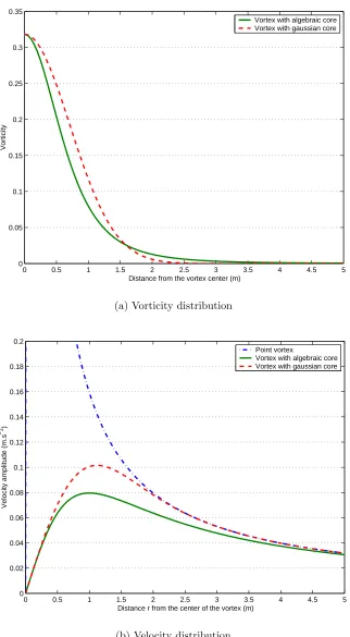
2.2 Comparison between different vortex cores . . . 50

2.3 Example of disposition for the panel method (courtesy of Takeda) . . . . 54

2.4 Wall approximation for straight panels . . . 58

2.5 Wall approximation for curved panels . . . 59

2.6 Illustration of the reflection used (courtesy of N.C.Clarke) . . . 73

2.7 Comparison of Cm for the Spalart simulation at α= 45, for different ∆t∗ 79 2.8 Comparison ofCm for the Spalart simulation atα= 45, for different ∆t∗ for a total number of vortices N = 6800 . . . 80

2.9 General algorithm . . . 85

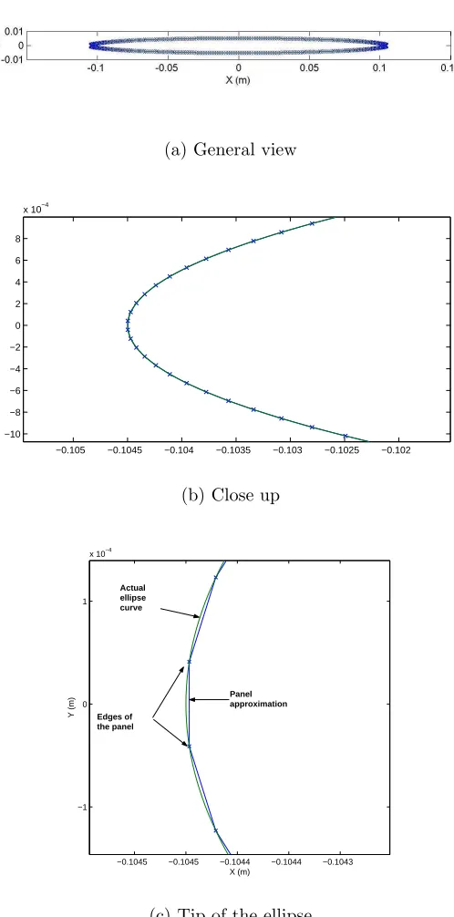
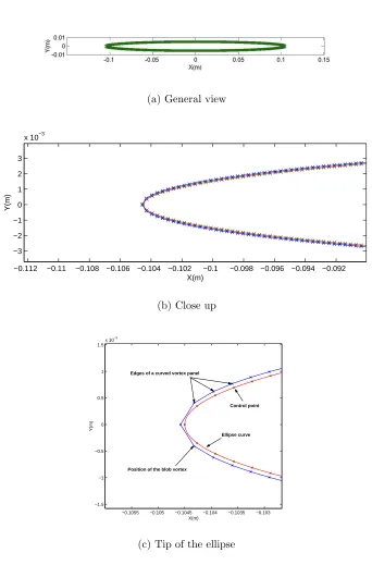
3.1 Streamline of a flow past a 20:1 ellipse for the blob vortex method . . . . 89

3.2 Streamline of a flow past a 20:1 ellipse for the potential flow solution . . 90

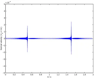
3.3 Log10(ε) distribution in the grid for the 20:1 ellipse and uniform translation 92 3.4 Logarithm of the normal velocity at the boundary for two incidence an-gles α . . . 93

3.5 Velocity and streamline between the boundary vortices and the wall for 90o _{incidence . . . 94}

3.6 Comparison of the velocity induced by the blob vortices (red vector) and the velocity from the exact potential solution (blue line). The wall is marked by a black line, and the boundary vortices are marked by green crosses. . . 94

3.7 Streamline of a flow past a 20:1 ellipse for the blob vortex method . . . . 95

(8)

3.9 Log10(ε) distribution in the grid for the 20 : 1 ellipse and uniform rotation 97 3.10 Normal velocity at the boundary . . . 98

3.11 Blob vortices plot for t∗ _{= 51}_._{5 and} _α _{= 50 with various global number}

of vortices N using the Spalart code. See figure 3.12 for the scale. . . 102

3.12 Scale for figure 3.11. . . 103

3.13 Cn for various angle of incidence and global number of vortices N . . . . 103

3.14 Ct for various angle of incidence and global number of vortices N . . . . 104

3.15 S for various angle of incidence and global number of vortices N . . . 104

3.16 Measures characterizing the flow . . . 105

3.17 Vortex plot at a given time step from the Spalart code. Vortex are blue crosses, the body is black, the direction of the ellipse motion is indicated

by the arrow . . . 107

3.18 Nascent vortices strength shed from the ellipse for α= 80o_{. The filter is} defined by equation 3.7. . . 109

3.19 Streamline of the flow for the Spalart code att∗ _{= 51}_._{5 with} _α_{= [45}_,₅₀_,_60]112 3.20 Streamline of the flow for the Spalart code att∗ _{= 51}_._{5 with} _α_{= [70}_,₈₀_,_90]113 3.21 Streamline of the flow for the C code at t∗ _{= 51}_._{2 with} _α_{= [45}_,₅₀_,_{60] . . 114} 3.22 Streamline of the flow for the C code at t∗ _{= 51}_._{2 for} _α _{= 70}o_, _t∗ _{= 40}

for α= 80o _and _t∗ _{= 72 for} _α_{= 90}o _{. . . 115}

3.23 Enlarged streamline plot at t∗ _{= 51}_._{5 for the Spalart code for} _α _{= 50}

(the black line represents the end of the streamline plots in fig 3.19 and

3.20) . . . 116

3.24 σ and (σ)√N influence on the Strouhal number for α = 50o _{using the}

Spalart code. Both variables units are in meter. . . 118

3.25 Normal and tangential force coefficients time plot for the Spalart code

with α = [45,50]o _{. . . 123} 3.26 Normal and tangential force coefficients time plot for the Spalart code

with α = [60,70]o _{. . . 124} 3.27 Normal and tangential force coefficients time plot for the Spalart code

with α = [80,90]o _{. . . 125} 3.28 Normal and tangential force coefficients time plot for the C code with

α = [45,50]o _{. . . 126} 3.29 Normal and tangential force coefficients time plot for the C code with

(9)

3.30 Normal and tangential force coefficients time plot for the C code with

α = [80,90]o _{. . . 128}

3.31 Streaklines and streamlines sequence for an impulsively started flat plate at Re = 200, α = 45o_{. The streamfunction values in (b) range from} [₋1.13, 1.13]_×(2a U_∞) with a concentration around 0 at t∗ _{= 6}_._{78 . . . . 135}

3.32 Force and moment coefficients for a stationary ellipse in a parallel freestream flow at 45 degrees with Re= 200 . . . 136

3.33 Force and moment coefficients for a rotating ellipse in a parallel freestream flow (for subfigure 3.33(b) the dotted line represents the forces and mo-ment coefficients from Lugt and Ohring). . . 137

3.34 Plot scale for the streamline plots in figure 3.35, 3.36 and 3.37. . . 138

3.35 See figure 3.37 for the caption and figure 3.34(a) for the scale. . . 139

3.36 See figure 3.37 for the caption and figure 3.34(a) for the scale. . . 140

3.37 Sequence of streamlines around a rotating ellipse in a parallel flow for Re = 200,Ro = 2, and an initial incidence of π/2. In contrast to every other sections, the freeflow is flowing from right to left. See figure 3.34 for the scale. . . 141

3.38 Illustration of the system ellipse and fluid . . . 143

3.39 Scale for the streamline plot in figures 3.45, 3.46, and 3.47. . . 154

3.40 Time evolution of the angle of the plateθfor a spring damped plate with f∗ n = 1/2, ξ∗ = 0 and starting with an initial angle θ0 =−1o. . . 155

3.41 Time evolution of the angle of the plateθfor a spring damped plate with f∗ n = 1/2, ξ∗ = 0 and starting with an initial angle θ0 = 1o. . . 156

3.42 Time evolution of the angle of the plateθfor a spring damped plate with f∗ n = 1/8, ξ∗ = 0 and starting with an initial angle θ0 =−1o. . . 157

3.43 Time evolution of the angle of the plateθfor a spring damped plate with f∗ n = 1/8, ξ∗ = 0 and starting with an initial angle θ0 = 1o. . . 157

3.44 Time evolution of the angle of the plateθfor a spring damped plate with ξ∗ _{= 0 and starting with an initial angle}_θ 0 =−2.5o. . . 158

(10)

3.46 Streamlines comparison of the flow for the Spalart code with θ0 = 1o

and f∗

n = 1/[2,8]. Streamfunction values range is [−0.066, 0.066] × (2a U_∞). It corresponds to [₋0.0423, 0.0423]_×(2a Umax) for fn∗ = 1/2, and [₋0.169, 0.169]_×(2a Umax) for fn∗ = 1/8 (Umax varies with fn∗ see equation 3.27). In both cases, values are concentrated around 0. See

figure 3.39 for the scale. . . 160

3.47 Streamline of the flow for the Spalart code with θ0 =−1o andfn∗ = 1/2. Streamfunction values range is [₋0.066, 0.066]_×(2a U_∞). It corresponds to [₋0.0423, 0.0423]_×(2a Umax). Values are concentrated around 0. See figure 3.39 for the scale. . . 161

3.48 Time plot of the angle evolution for f∗

n = 1/4 with various ξ∗ . . . 165

n = 1/8 with various ξ∗ . . . 166

n = 1/11 with various ξ∗ . . . 166

3.51 Angle evolution θ(t) and PSD plot for θ∗ _and _C

m (for t∗ = [12.8,204.8]) in the case ξ∗ _{= 0}_._{02 and 1}_/f∗

n = 4. The crosses in the PSD are the main

harmonics represented in θ∗₍_t_{) . . . 168}

n = 11. The crosses in the PSD are the

main harmonics represented in θ∗₍_t_{) . . . 171} 3.55 Scale plot for figures 3.57, 3.58, 3.56, 3.59, 3.61, 3.62, 3.64, 3.65 . . . 173 3.56 History of θ and Cm in phase C for 1/fn∗ = 4 . . . 174 3.57 Streamlines for the flow in phase C for 1/f∗

n = 4 with t∗ = [174.8,178.3] (see figure 3.56). The scale is in figure 3.55. . . 175 3.58 Streamlines for the flow in phase C for 1/f∗

n = 4 with t∗ = [178.8,182.3] (see figure 3.56). The scale is in figure 3.55. . . 176

3.59 Streamlines for the flow in phase C for 1/f∗

n = 4 with t∗ = [182.8,184.3] (see figure 3.56). The scale is in figure 3.55. . . 177

(11)

3.61 Streamline for the flow in phaseC for 1/f∗

n = 7 witht∗ = [135 138.4] (see

figure 3.60). The scale is in figure 3.55. . . 180

3.62 Streamline for the flow in phaseC for 1/f∗ n = 7 witht∗ = [139 142.4] (see figure 3.60). The scale is in figure 3.55. . . 181

3.63 History of θ and Cm in phase C for 1/fn∗ = 11 . . . 184

3.64 Streamline for the flow in phase C for 1/f∗ n = 11 witht∗ = [154.8 158.3] (see figure 3.63). The scale is in figure 3.55. . . 185

3.65 Streamline for the flow in phase C for 1/f∗ n = 11 witht∗ = [158.8 162.3] (see figure 3.63). The scale is in figure 3.55. . . 186

3.66 Summary of the simulations detailing the variations of the shedding fre-quency f∗ s and the maximum amplitude of angle oscillation regarding the nondimensional natural frequency f∗ n . . . 189

3.67 Mean values and root mean square ofCn depending on 1/fn∗ . . . 192

3.68 Mean values and root mean square ofCt depending on 1/fn∗ . . . 193

3.69 Mean values and root mean square ofCm depending on 1/fn∗ . . . 194

4.1 Plan for the system modeling . . . 203

4.2 Starting transfer functions for the magnitude and frequency interpolation in figure 4.3. . . 205

4.3 Magnitude interpolation only compared to magnitude and frequency in-terpolation for a constant input xr. Functionsf1 and f2 are presented in figure 4.2. . . 206

4.4 Example of simulation time range retained . . . 208

4.5 General diagram for identification method (courtesy of G.Zwingelstein) . 209 4.6 General example for fuzzy logic . . . 210

4.7 Fuzzy set for u1 . . . 211

4.8 Fuzzy set for u2 and y . . . 212

4.9 Example of inference table . . . 213

4.10 Example of inference for one fuzzy rule . . . 214

4.11 Results from all the fuzzy rules, and aggregation . . . 215

4.12 Defuzzification using the centroid method . . . 216

4.13 General linear model for the flow at a steady angle . . . 223

(12)

4.15 Validation results for a plate with steady incidence angles α = 60, 70

degrees . . . 225

4.16 Validation results for a plate with steady incidence angles α = 80, 90 degrees . . . 226

4.17 Global model for the plate at steady angles . . . 229

4.18 Frequency and mean interpolation function . . . 230

4.19 Membership functions of α . . . 232

4.20 Comparison between simulation and steady plate model for α = 55 de-grees, output history plot. . . 234

4.21 Comparison between simulation and steady plate model using a peri-odogram. PXX is the power spectral density (PSD) of the signalx(t) or –for this figure– Cm. . . 234

4.22 Plate dynamics model . . . 235

4.23 Coupled plate and flow model Bode diagram at α = 50o _{using polystyrene238} 4.24 Coupled plate and flow model Bode diagram at α = 50o _{using aluminium 239} 4.25 Coupled plate and flow model Bode diagram at α = 60o _{using polystyrene240} 4.26 Coupled plate and flow model Bode diagram at α = 60o _{using aluminium 241} 4.27 Coupled plate and flow model Bode diagram at α = 70o _{using polystyrene242} 4.28 Coupled plate and flow model Bode diagram at α = 70o _{using aluminium 243} 5.1 Coupled plate and flow model . . . 249

5.2 Controller, Coupled plate and flow model . . . 250

5.3 Classical based, linear controller block diagram . . . 256

5.4 Control and system closed loop block diagram for the classical controller. 256 5.5 Output of the closed loop system for a step input for the classical controller.259 5.6 Error of the closed loop system for a step input for the optimal controller.260 5.7 Control signal evolution in time for the classical controller (the verti-cal line is actually a control input peak due to the step input). Cf Ce definition in eq. 5.19. . . 261

5.8 Control signal evolution in time for the classical controller without taking into account the torque due to the spring. Cf Ce definition in eq. 5.19 for the non-dimensionalization. . . 262

5.9 Power signal evolution in time for the classical controller. The power is divided by (1/2)ρU3 ∞L . . . 263

(13)

5.11 Control and system closed loop block diagram for the optimal controller. 271 5.12 Output of the closed loop system for a step input for the optimal controller.271

5.13 Error of the closed loop system for a step input for the optimal controller.272 5.14 Control signal evolution in time for the optimal controller (the

verti-cal line is actually a control input peak due to the step input). Cf Ce

definition in eq. 5.19. . . 273

5.15 Control signal evolution in time for the optimal controller without taking

into account the torque due to the spring. Cf Ce definition in eq. 5.19

for the non-dimensionalization. . . 274

5.16 Power signal evolution in time for the optimal controller. The power is divided by (1/2)ρU3

∞L . . . 275 5.17 Membership functions of the input . . . 277

5.18 Inference table for the fuzzy control . . . 278 5.19 Control and system closed loop block diagram for the fuzzy logic controller.284

5.20 Output of the closed loop system for a step input for the fuzzy logic

controller. . . 285 5.21 Error from the optimal controller minus the error from the fuzzy

con-troller with relative calculus precision of 10−6_{. . . 285}

5.22 Error of the closed loop system for a step input for the fuzzy logic controller.286 5.23 Control signal evolution in time for the fuzzy logic controller (the

verti-cal line is actually a control input peak due to the step input). Cf Ce

definition in eq. 5.19. . . 287

5.24 Control signal evolution in time for the fuzzy logic controller without

taking into account the torque due to the spring. Cf Ce definition in eq.

5.19 for the non-dimensionalization. . . 288

5.25 Power signal evolution in time for the fuzzy controller. The power is divided by (1/2)ρU3

∞L . . . 289 5.26 Control signal and angular error evolution in time for the fuzzy logic

controller with relative calculus precision of 10−6_{. Cf}_C

e definition in eq.

5.19 for the non-dimensionalization. . . 290

5.27 Power signal evolution in time for the fuzzy controller with relative

cal-culus precision of 10−6_{. The power is divided by (1}_/₂₎_ρU3

∞L. . . 291 5.28 Control and system closed loop block diagram for the optimal controller

(14)

5.29 Time plot of the angle evolution and controller torque input for the

flow/plate system controlled by the fuzzy logic controller with f∗

n = Ss

and ∆t∗ _{= 0}_._{05 . . . 299} 5.30 Time plot of the angle evolution and torque input for the flow/plate

system controlled by the fuzzy logic controller with f∗

n = 1.5Ss and

∆t∗ _{= 0}_._{05 . . . 300} 5.31 Time plot of the angle evolution and torque input for the flow/plate

system controlled by the optimal controller with f∗

n =Ss and ∆t∗ = 0.04 301 5.32 Time plot of the angle evolution and torque input for the flow/plate

system controlled by the optimal controller withf∗

n = 1.5Ssand ∆t∗ = 0.04302 5.33 Time plot of the angle evolution and torque input for the flow/plate

system controlled by the optimal controller with f∗

n =Ss and ∆t∗ = 0.05 303 5.34 Time plot of the angle evolution and torque input for the flow/plate

n = 1.5Ssand ∆t∗ = 0.05304 5.35 Time plot of the angle evolution and torque input for the flow/plate

n = 1.5Ssand ∆t∗ = 0.05305

5.36 Time plot of the angle evolution for the flow/plate system withf∗

n =Ss, ∆t∗ _{= 0}_._{05 and the fuzzy-logic controller enabled at}_t∗ _{= 51}_._{2 . . . 306}

5.37 Time plot of the torque input for the flow/plate system with f∗

n = Ss, ∆t∗ _{= 0}_._{05 and the fuzzy-logic controller enabled at}_t∗ _{= 51}_._{2 . . . 307} 5.38 Time plot of the angle evolution and torque input for the flow/plate

system with f∗

n = Ss, ∆t∗ = 0.05 and the fuzzy-logic controller enabled at t∗ _{= 51}_._{2 during transition . . . 308} 5.39 Time plot of the angle evolution for the flow/plate system motion

con-trolled by the fuzzy-logic controller with f∗

n=Ss . . . 316 5.40 Time plot of the angle evolution for the flow/plate system motion

n= 1.5Ss . . . 316 5.41 Time plot of the error evolution for the flow/plate system motion

n=Ss . . . 317 5.42 Time plot of the controller torque input for the flow/plate system motion

controlled by the fuzzy logic controller with f∗

n =Ss . . . 318 5.43 Time plot of the power signal evolution in time for the fuzzy logic

con-troller with f∗

n =Ss. The power is divided by (1/2)ρU_∞3L. . . 319 5.44 Time plot of the error evolution for the flow/plate system motion

(15)

5.45 Time plot of the controller torque input for the flow/plate system motion controlled by the fuzzy-logic controller with f∗

n = 1.5Ss . . . 321 5.46 Time plot of the power signal evolution in time for the fuzzy logic

n = 1.5Ss. The power is divided by (1/2)ρU_∞3L. . . 322 5.47 Time plot of the angle evolution for the flow/plate system motion

con-trolled by the optimal controller with f∗

n =Ss . . . 323 5.48 Time plot of the angle evolution for the flow/plate system motion

n = 1.5Ss . . . 323 5.49 Time plot of the error evolution for the flow/plate system motion

n =Ss . . . 324 5.50 Time plot of the torque input for the flow/plate system motion controlled

by the optimal controller with f∗

n =Ss . . . 325 5.51 Time plot of the power signal evolution in time for the optimal controller

with f∗

n =Ss. The power is divided by (1/2)ρU_∞3L. . . 326 5.52 Time plot of the error evolution for the flow/plate system motion

n = 1.5Ss . . . 327 5.53 Time plot of the torque input for the flow/plate system motion controlled

n = 1.5Ss . . . 328 5.54 Time plot of the power signal evolution in time for the optimal controller

with f∗

n = 1.5Ss. The power is divided by (1/2)ρU_∞3 L. . . 329 5.55 Time plot of the angle evolution for the flow/plate system motion

n=Ss and oscillating input . . 335 5.56 Time plot of the angle evolution for the flow/plate system motion

n= 1.5Ss and oscillating input 335 5.57 Time plot of the error evolution for the flow/plate system motion

n=Ss and oscillating input . . 336 5.58 Time plot of the controller torque input for the flow/plate system motion

controlled by the fuzzy logic controller with f∗

n =Ss and oscillating input 337

5.59 Time plot of the power signal evolution in time for the fuzzy logic con-troller with f∗

n = Ss and oscillating input. The power is divided by

(1/2)ρU3

∞L. . . 338 5.60 Time plot of the error evolution for the flow/plate system motion

(16)

5.61 Time plot of the controller torque input for the flow/plate system motion controlled by the fuzzy-logic controller with f∗

n = 1.5Ss and oscillating input . . . 340 5.62 Time plot of the power signal evolution in time for the fuzzy logic

n = 1.5Ss and oscillating input. The power is divided by

(1/2)ρU3

∞L. . . 341 5.63 Time plot of the angle evolution for the flow/plate system motion

n =Ss and oscillating input . . . 342

5.64 Time plot of the angle evolution for the flow/plate system motion

n = 1.5Ss and oscillating input . . 342 5.65 Time plot of the error evolution for the flow/plate system motion

5.66 Time plot of the torque input for the flow/plate system motion controlled by the optimal controller with f∗

5.67 Time plot of the power signal evolution in time for the optimal controller

with f∗

n =Ss and oscillating input. The power is divided by (1/2)ρU_∞3L. 345 5.68 Time plot of the error evolution for the flow/plate system motion

n = 1.5Ss and oscillating input . . 346 5.69 Time plot of the torque input for the flow/plate system motion controlled

n = 1.5Ss and oscillating input . . . 347 5.70 Time plot of the power signal evolution in time for the optimal controller

withf∗

n = 1.5Ssand oscillating input. The power is divided by (1/2)ρU_∞3 L.348 C.1 Conformal transformation illustration . . . 365

C.2 Complex decomposition of contour . . . 367

(17)

I would like to thank first and foremost Dr Gary N Coleman for supervising this work, and especially for his sound advice and his comprehension over the years. Also

many thanks to Dr Owen R Tutty for his technical help as an advisor and his frankness.

I am grateful too to the Aeronautics and Astronautics department staff as well as the University of Southampton for funding my work.

There have also been many other collaborators to which I’m indebted. Professor Sergei

I Chernyshenko for having enlightened me on Complex problems and certain flow con-cepts; Doctor Kenji Takeda for his help on the previous vortex method research in the

department; Professor Philippe Spalart for having given some insight, and sparking

some interests on the vortex method as well as for helping me with the numerical flow method. I also want to thank the many people which I’ve known in my years in the

University and the colleagues who passed over the years who have always supported me

(in an english and french sense) among those David Simonin, Ajay N Modha, Sandrine Morin, Cary Turagan, A. Bouferrouk, Joanna Hyde, Anne Roques and many other

peo-ple.

Finally, special thanks to my wife who has born part of the burden during this thesis

(18)

(−→X,−→Y ) Stationary frame during the motion centered in O(0,0)

α Ellipse incidence angle or angle of attack

α0 Incidence angle of the ellipse at t= 0

¯

x Mean value of x

∆Γ Rate of vorticity

∆θ Angular error

δN Distance between a boundary vortex and the corresponding boundary control

point

∆t Timestep (Note : sometimes referred to as dt or dt in graphics)

δ Two-dimensional Dirac delta function

δ0 Average distance between the control points on the boundary

δbl Boundary layer thickness

Distance of the nascent vortex to the body when using the discrete introduction

of vorticity method

Γ Strength of a discrete vortex or circulation

γ Vorticity distribution or vortex core function

Γb Circulation on the boundary

Γf Wake circulation

µ Torsional damping of the spring damped ellipse sometimes referred to as b in

(19)

µs Effective damping of the spring-damped ellipse system using alternative nondi-mensionalization (see section 3.3.1 for mathematical definition)

∇ Gradient operator

ν Kinematic viscosity

Ω Body angular velocity

ω Magnitude of −→ω

−

→_ω _{Vorticity of the fluid}

− →

Fs Smoothed aerodynamic force

− →

F Aerodynamic force

−

→_f _{Body force per unit mass}

−

→_K _{unit vector orthogonal to the (}₋_→_{x ,}₋_→_y _{) plane} −

→_n _{Unit vector normal to the wall}

−

→_P _{Point position in a flow domain}

−

→_s_b _{Position vector defining the location of the surface boundary}

−

→_s _{Unit vector tangential to the body surface}

−→

U_∞ Freestream flow velocity vector

− →

un Normal velocity component on the boundary

− →

uo Initial velocity field

− →

us Tangential velocity component on the boundary at −→x =−→sb

−

→_u _{Fluid velocity}

− →_U

e External flow velocity

−

→_v_s _{Body velocity}

−

→_V _{= (}_{u, v}_{) Velocity vector with} _u _and _v _{respectively the} ₋_→_x _and ₋_→_y _{axis component} −

→

(20)

− →

xv Discrete vortex position in a flow domain

−

→_x _{major axis of the ellipse (can also denotes a position)}

−

→_y _{minor axis of the ellipse}

Φ Velocity potential in a stationary frame

ψ Streamline function

ψ∞ Stream function from the uniform freestream velocity

ψb Stream function associated to the boundary vortices

ψf stream function coming from the flow vortices

ψr Streamfunction due to the rotation

ρ Fluid mass per volume unit

ρb Body mass per volume unit

σ Cut-off radius, or vortex core radius

θ(t) Angular position of the plate from the rest position of the torque spring, α =

α0+θ(t) and Ω = ˙θ

θ0 Initial ellipse spring angle

θi Angle determining the position of the ith boundary vortices in chapter 2

θmax Maximum θ oscillations amplitude

E External disturbance vector

Rc Reference command signal

Rv Covariance of V

Rw Covariance of W

U Input vector of system

V Sensor noise

(21)

Xc Controller state vector

X State vector of system

Y Output vector of system

ε(x, y) Error at a point of position (x, y) (noted in figures)

εp Position error

εv Velocity error

$n Natural frequency of the spring damped ellipse in rad/s

ξ Reduced damping of the spring damped ellipse

ξ∗

s Nondimensional effective ξ of the θ(t) produced by the coupled mechanical/flow

system

ζ Complex position in a circle plane (before a Joukowski transformation) for

ex-ample

ζ0 _{Complex value of the location of an image vortex in the} _ζ _plane

ζ∗ _{Conjugate of a complex position in a circle plane}

a Ellipse half chord on its primary axis

b Half chord of the ellipse on the minor axis

c Half the chord value or radius of the circle in the complex image plane

Ca Torque output of the controller, scalar dependent on time

Cd Aerodynamic drag coefficient

Ce Non-dimensionalized torque output of the controller (see equation 5.19), scalar

dependent on time.

Ce Nondimensional external torque provided by Simulink to the C flow simulation

CG= 1/k Steady-state gain of the transfer function. (see section 3.3 for mathematical

(22)

CJ Additional mass to the spring-damped ellipse system (see section 3.3.1 for math-ematical definition)

Cl Aerodynamic lift coefficient

Cma Approximated Cm

Cm Aerodynamic moment coefficient

Cn Aerodynamic normal force coefficient (associated to the −→y axis)

Cp incident flow power impinging on the plate of chord L. It is defined by Cp =

(1/2)ρ U3

∞L for a 2D plate.

Ct Aerodynamic tangential force coefficient (associated to the −→x ellipse axis)

D Entire flow domain

D0 Ad hoc Spalart simulation parameter: length parameter that allows one to obtain

better resolution near the wall

D% Peak response in percent

e Error signal (input of the fuzzy logic controller), scalar dependent on time

Ec,p(T1, T2) Energy provided by Pc∗ between T1 and T2 (see equation 5.9)

Ec,p(T1, T2) Signal energy provided by Pc∗ betweenT1 and T2 (see equation 5.9)

Ec(T1, T2) Energy used by the controller betweenT1 and T2(see equation 5.3)

Es(T1, T2) Signal energy of the controller betweenT1 and T2(see equation 5.5)

F(s) Laplace transform of a function f(t)

f(t) Generic function dependent on time when applied to a control system

fθ θ oscillation frequency for the coupled spring damped ellipse/flow system

fm Flow linear model main harmonics frequency

f∗

n,s Nondimensional effectivefnof theθ(t) produced by the coupled mechanical/flow

system

(23)

fsamp Sampling frequency

fs Flow vortex shedding frequency

h Length of a square cell in a uniform grid defining the approximate flow domain

simulated

J Angular inertia of the spring damped ellipse

J∗

s Effective nondimensional inertia of the spring-damped ellipse system (see section

3.3.1 for mathematical definition)

k Torsional spring coefficient applied of the spring damped ellipse, exceptionally

generic scalar in section 4.3.3

L Ellipse Chord

M Aerodynamic moment

Me External torque provided by Simulink to the C flow simulation

mf x Generic name for membership function for fuzzy logic controller

N Total number of discrete vortices

Nb Number of boundary vortices

O orO(0,0) Origin

p pressure

Pb Set of parameters defining the position and orientation of a boundary element

Pc Instantaneous power used by the controller (see equation 5.2)

PXX Signal power per frequency in the spectrum considered for a time signal x(t).

This is related to the signal power not the physical power. The units of PXX

is that of x2_{. The power spectral density (PSD) designates the} _P

XX considered

over the whole spectrum.

Q State penalty matrix

R Cost penalty matrix

(24)

Rs Region occupied by the solid body

Ro Rossby number, Ro=U_∞/(aΩ)

S Strouhal number or Strouhal number extracted from experiment

Sbody Cross section surface of a body

Ss Actual Strouhal number extracted from previous simulation

T A duration value

t Real timescale or time value

t0 _{Alternative timescale}

t5% Minimal settling time

tr Minimal rise time

u Input signal of a system, or output signal of a controller (scalar form)

U_∞ Magnitude of the uniform freastream velocity or uniform freastream complex

velocity

Umax Maximum angular velocity of the spring damped ellipse system in vacuum (see

section 3.3.1 for mathematical definition)

Ush Shear layer velocity magnitude

uX −→X velocity component of −→u

uY −→Y velocity component of −→u

V0 Ad hoc Spalart simulation parameter: tolerance parameter for blob vortex

merg-ing adjustment

V1 Velocity magnitude at the outer edge of the shear layer

V2 Velocity magnitude at the inner edge of the shear layer

w complex flow potential

wf Freeflow complex potential

(25)

xj(t) Position of the jth discrete vortex

y Output signal when applied to a control system (scalar form)

(−→x,→−y) Body fixed frame of reference

* Convolution operator

Re Reynolds number

Subscript b Associated to the boundary vortices

Subscript e Associated to the estimator (when applied to control system)

Subscript p Associated to the vortices with positive circulation in the method with

discrete introduction of vorticity

Subscript q Associated to the vortices with negative circulation in the method with

discrete introduction of vorticity

Subscript w Associated to the vortices released in the flow

Superscripts ∗ _{Nondimensionalized variable (except for complex variables)}

(26)

Introduction

1.1 General overview

Many engineering devices involve the interaction of a flexible structure and a moving fluid. In some cases this interaction is dynamic, with the deflected structure altering the

original flow pattern - and the altered flow pattern then re-deflecting the structure and

so on. Accurate analysis of these cases requires a careful multi-disciplinary approach. They also provide a challenging test for active control strategies. With this project, a

study is made about a rotating rigid plate in a transverse crossflow. By considering

an idealized fluid-structure interaction, an integrated fluid, structure and active control analysis is developed, which is expected to be relevant to the more complicated

situa-tions found in practice.

In order to investigate the flow around the plate, whether stationary or rotating about

an axis normal to the flow, a CFD method is implemented. The main aim is to

de-sign a method simple enough to avoid using too much computer power, but accurate

enough to model realistically the flow pattern and the flow forces. Therefore, a 2D (2

dimensional) blob vortex method has been chosen for modeling the unsteady wake. The

position and the strength of the nascent vortices are able to vary with time through the

use of the Kutta condition.

The flow simulation will enable investigations of the effect of the moving plate on

(27)

The goals of the project are :

• Study the flow past a rotating rigid flat plate in different configurations (steady

inclination, oscillating between two inclinations, or rotating)

• Validate the blob vortex method with a rotating body

• Investigate the strategies and limits of a control scheme for this test case

1.1.1 Objectives

The main objective of this project is the control of a flat plate placed in a

trans-verse unbounded flow, with angle of attack ranging from 45 to 90 degrees. The fluid is

assumed to be incompressible. The plate is assumed to be perfectly rigid, and bending

and vibration of the structure are ignored.

Figure 1.1: General scheme

The plate will be held fixed in some cases and in others allowed to rotate about a central

axis, with a torsional spring and damper to resist the motion. This will illustrate the

feasibility and the limitations of this approach applied to similar flows.

Although this project remains fairly idealized, it is intended to act as a preliminary

for studies of more realistic real-world flows, such as that around a moving spoiler on

(28)

1.1.2 Systems

Several systems are to be implemented to achieve the full simulation. These include

the 2D flow simulation and modeling, the computation of the dynamics of the rigid

plate, and the control. The control part will be implemented in Matlab, whereas the

flow and kinematics parts will be implemented in C/C++.

1.1.2.1 2D Dynamic flow simulation

First of all, a simple flow simulation is considered, that is to say in a way that could allow not only the coupling with the control, but also good computational speed. It is

also necessary here that the simulation algorithm can be readily modified. However,

the simulation must still be also be able to produce realistic flow characteristics, for example the Karman Street in the case of the fixed plate. Therefore, a vortex method

was chosen as the most appropriate method, since it is ideal for simulating separated

bluff-body flows.

For the programming language, C/C++ was used for reasons of computational speed

and availability. A first implementation has been done in Matlab to settle the algorithm.

1.1.2.2 Plate motion

Using classical mechanics equations and the input forces from the 2D flow

simula-tion, one can then deduce the movement of the plate. A homogeneous rigid plate is

considered with mass density corresponding to Plexiglass.

This part will also be coded in C/C++ as a module for the 2Dflow simulation.

1.1.2.3 Control

Considering now the control part, it must ensure numerous roles, among which are

the control of the angle of attack as a function of time. In addition, the plate stabiliza-tion has to be achieved. Finally, for this project, the flow simulastabiliza-tion and the control

must communicate at each iteration. Matlab was chosen as there are a number of tools

(29)

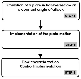
1.1.3 Methodology

The methodology consists of three steps. At each step, an assessment is done to validate the completed part. The first part will be dedicated to the implementation

of the vortex method with a fixed plate in a crossflow. In the second part, the plate

will rotate freely around a given axis under the flow action. Finally, the third step will

consist of the implementation of the control as well as the development of a system model of the plate and the flow.

Although this type of implementation does not provide optimal computational speed, it enables to simplify the debugging as well as giving flexibility if the configuration of

the system needs to be changed.

The first two steps provide the flow simulation, whereas the third gives the control.

It should be noted that between the control part and the simulation part, the input

[image:29.595.197.461.460.719.2]

and output were to be as simple as possible in order to keep these two parts independent.

(30)

1.1.4 Integration

The simulation and the control need to be integrated. As previously stated, the flow simulation will be implemented in C/C++, and the control part in Matlab. Therefore,

several approach are possible, namely :

• To use a file as an interface between C/C++ and Matlab. At each time step, the

flow simulation generates a file containing all the useful data of the flow for use by the control. In Matlab, this file is then read, and create a file as an input for

the flow simulation after having determined the resulting control.

• To implement a program in either C/C++ or Matlab to handle the data as well

as dynamically determine the interaction between the flow simulation and the

control.

The first approach is the easiest, but is intrinsically slower than the second option. Furthermore, it requires careful synchronization between C and Matlab. On the other

hand, the second approach requires a driver to couple both parts (C/C++ and Matlab).

The main implementation difficulty consists in using an intermediary function to enable the simulation and Matlab to share data through a common data structure. Thus, this

driver implementation needs little modification of both parts. Therefore, the second

approach was preferred to integrate the Matlab controller and the C simulation.

1.2 Literature review

1.2.1 Overview

As standard methods will be used for the control (linear systems, system modeling,

etc), the literature review will be oriented toward the vortex method. Nevertheless,

some papers have appeared on the subject of vibrating plates (no aerodynamics in-volved), or of flap of a wing. A brief review of these studies is provided in the third

section.

The vortex method is widely used in research, mainly because of its ability to

cre-ate physically relevant dynamics at high Reynolds number. Consequently, there is an

extensive literature on the subject; one of the most exhaustive papers is by Sarpkaya

(31)

work for a comprehensive review, while here are the papers which are more significant for the current project purposes.

This review is divided into three sections. The first considers papers on the complete

vortex method, i.e. providing the theoretical and computational tools to develop and

implement the method. The second section introduces different schemes available as

part of the vortex method. The third section focuses on some of the schemes available for controlling motion in structural and mechanical problems.

1.2.2 Guiding papers

The most used papers, as well as the most extensive in their review, are those of

Spalart (1988) [57], Sarpkaya (1994), Leonard (1980) [33], and Chorin (1993) [10]. One

should also take into account the books of Katz and Plotkin (1991) [30] and Kout-soumakos (2000) [13].

The Chorin paper [10] exposes some of the theoretical aspects of the discrete vortex method in two and three dimensions. Although very useful for convergence and error

study, it does not provide the material necessary for constructing the method. The

Koutsoumakos book [13] has the same scope albeit more comprehensively. It studies increasingly complex cases including hybrid schemes (finite difference on the boundary,

vortex difference for the far field). Koutsoumakos also provide some scope over the

parameters for convergence of the method.

Leonard [33] presents a complete review on the method which is more oriented

to-ward application. He exposes some of the problems such as the accuracy of convection

schemes, the determination of an appropriate blob shape, and the viscosity problem,

as well as some test cases. He also considers the 3D (3 dimensional) case. It has been

found very useful since he discusses how to set the ad-hoc parameters (vortex core

ra-dius, time step, minimum number of vortices to use) and presents an explanation about convergence. However, not enough details are provided for a full implementation of the

method.

(32)

complicated body shapes. The paper is “recipe book” giving details of the implemen-tation of the discrete vortex method. There is even a part dedicated to the efficient

programming of the method.

Sarpkaya (1994) [53] is a thorough review paper about the different schemes in use.

He first develops the mathematics related to the method, and discusses the different

schemes in chronological order. He then gives a great deal of detail about each of them. Compared to other papers, this review is oriented toward an engineering point of view.

Katz and Plotkin (1991) [30] in their book provide a useful background for the

ele-ments method in general (discrete source, discrete vortices, 2D and 3D). Although it

is lacking some details about the schemes, like the Spalart paper it is a “recipe book”

with an engineering perspective. Therefore, it is a good starting point for the under-standing and implementation of discrete methods. It does not however discuss blob

vortex methods.

1.2.3 Discrete vortex schemes

Numerous vortex methods have been devised for steady as well as unsteady flows.

Here is not an exhaustive review of the various methods but rather a concise presenta-tion of the most representative ones. The flow configurapresenta-tion considered in this project

(transverse flow over a flat plate) is incompressible, inviscid and with separation.

Most flows treated are incompressible. The compressible case are not reviewed here; it

is discussed in references [1], [2], [6], [8], [20] and [57] on.

Sarpkaya (1974) [50] used an image method to model the flow around a transverse flat plate. Unlike the preceding papers, the shedding of vorticity is done discretely at

the separation points. He obtained some fairly good results, qualitatively speaking. He

conducted some further studies with the scheme being applied around a cylinder [49], and plates with a parabolic leading edge [52].

Koutsoumakos and Shiels [32] uses a Vortex In Cell (VIC) method and a Particle Strength Exchange (PSE) scheme to model the flow around an impulsively started

(33)

details. Their results agree well with experiment and yield insight into some of the effects observed.

Blevins (1991) [7] used a code developed by Spalart and Leonard (discrete vortex with

a surface distribution for the vortices, random walk method to account for viscosity) to

simulate flow around moving structures in an unbounded domain. Results show fairly

good agreement with experiment for the mean lift and drag. However, their worth is mostly qualitative as the phase and amplitude of the vortex shedding were

overpre-dicted.

Clarke (1992) [11] developed a discrete vortex method for simulating the flow around a

cylinder, using for the viscosity model a combination of diffusion velocity near the wall,

and random walk away from the wall. He also managed to run the simulation with a rotating cylinder, and conducted some long-term simulation for Reynolds number

rang-ing from 5000 to 31700, with good experimental agreement.

Takeda (1998) [59] did similar work but using viscosity distribution method to

ac-count for viscosity. The method is similar to a PSE method but differs in that there

is no regular regriding. He employed a highly parallel code. Like Clarke, he obtained high-quality results.

Most recently, Shiels (1998) [56] proposed a viscous vortex method based on blob vortex

core expansion. He applied this method to a transversely moving cylinder and spec-ified various means of computing the fluid forces. Although his simulation captured

the behaviour accurately enough to be confident that the dominant flow structures are

properly resolved, the accuracy at small scales is in doubt.

1.2.4 Vortex shedding phenomenology

The focus of this thesis requires an understanding of the interaction of the plate/flow system, and such the behavior of the basic flow. Thus, a review was made based on

studies of vortex-street and periodic flow phenomena. The scope of these studies is a

(34)

Marris (1964 [37]) provides a survey of research about periodic wakes behind a cylin-der in a uniform steady stream and is a synopsis of knowledge of the vortex formation

and of the associated hydrodynamic forces for a wide range of Reynolds numbers. He also discusses characteristics of the induced vibration in a uniform stream for various

spring-mounted bluff bodies configurations, and then focuses on the cylinder case.

Af-ter analyzing the vortex wake behind a cylinder at low Reynolds number of Re <300,

he concludes that the shedding process is associated with a deep low-pressure valley immediately aft of the cylinder. This implies that this low pressure area can be

re-moved by means of a splitter vane, which in turn stops the vortex shedding. He begins

with analysis on flow-induced vibration on the cylinder. He noted that self excitation can occur when bodies are rounded such that the boundary-layer separation points can

move on the body surface, emphasizing the role of the position of the separation point.

When self excitation does occur, the crossflow velocity is no longer negligible in relation to the streamwise velocity.

Berger and Wile (1972 [15]) also provide an extensive review of periodic flows. They note that, following Bearman, in an attempt to predict vortex-street parameters for

various body form, Kronauer proposed that for any vortex velocity the vortex street

set itself so as to reach the minimum drag due to the vortex formation, thus departing from Von Kalman’s idea based on stability theory. Among others, Gerrard (1966 [14]),

in a study of vortex formation behind bluff bodies, proposed the shedding frequency

scale is determined by two characteristics lengths: the length of the formation region,

and a length termed diffusion length. The first length simply stresses the importance of the entrainment of fluid from the interior of the formation region of vortices behind the

bluff body and its replenishment by reversed flow. The diffusion length represents the

thickness of the shear layer at the end of the formation region where the layer is drawn across the wake. He also observed that the Strouhal number for vortex shedding with

different freestream turbulence levels is almost independent of the Reynolds number.

The vibrating cylinder problem, although usually discussed in terms of 3D flow

fea-tures, offers several reflexions. First, the system consisting of an obstacle and a

peri-odic wake behaves like a nonlinear self-excited oscillator under forced vibration. Thus, aspects of a nonlinear system formed by an elastic solid body and fluid wake include

“synchronization” (lock in), hysterisis, frequency demultiplication, and in certain cases

(35)

oscillating cylinder and its periodic wake.

Other studies of interaction between a vortex street and bluff bodies and the oscil-lations induced on the bluff body have been done by Bearman (1984 [61]) and more

practically by Sarpkaya (1979 [55]). They highlight the difficulties in establishing a

mathematical model for the coupled flow/body system and stress the need for a

com-plete simulation model. Sarpkaya [55] focuses mainly on a numerical study, providing results for a cylinder oscillating transversely in a uniform stream using discrete

intro-duction of vorticity. Bearman [61], on the other hand, is more general and also analyzes

the fixed body case.

Lugt was involved in two studies investigating the flow around an ellipse using a

streamfunction-vorticity scheme for the Navier-Stokes equations, with both a steady and rotating ellipse. The first, with Haussling in 1974 [25], focused on the steady

el-lipse at 45 degrees angle of attack with thickness ratios from 1 to 0.1 and Reynolds

numbers ranging from 1 to 200. They found that similarly to the cylinder case, when

Re > 45 the steady state becomes unstable and the flow changes to a Karman

vor-tex street. Also, at Re = 200, the inertial effects of the flow were more pronounced

than at Re= 15 and 30. Those inertial effects manifests themselves in a distortion of

the vorticity generation and spreading close to the body, compared to the steady state

solution. At this Reynolds number, they noted the zero streamline is parallel to the

chord of the ellipse, which is a manifestation of the Kutta condition for viscous flow.

The period of the drag and lift coefficient history coincides with the vortex shedding. Effects of pressure dominate over those of friction. The maximum aerodynamic force

coefficients occur when the recirculatory region is the largest, which marks the end of

the roll-up of vorticity and the beginning of the vortex shedding. This state is charac-terized by a vorticity extremum. There is also a small maximum in the drag coefficient

emerging from the pressure influence and resulting from the proximity of the recently

shed vortices.

A moving ellipse study was carried out by Lugt and Ohring [26]. It involved an

el-lipse of lengtharotating at constant angular velocity at a Reynolds number of 200. To

characterize the angular velocity −→Ω compared to the freestream flow −→U_∞, they used the Rossby number (_|−→U_∞|/(_|−→Ω_|.a)). The flow was studied from the transient phase until

(36)

periodic behavior where two vortices are shed at each cycle. At this stage, the minimum for the moment coefficient in a cycle occurs when four recirculatory regions exist, i.e.

two suction regions under and above the surface of the ellipse which cancel each other, with the others at the tip of the ellipse acting in an antisymetric manner.

Ohmi et al [45] did an experimental and numerical investigation of an elliptic

cylin-der with high angle of attack (in the static stall regime, 15 to 45 degrees ). They considered the effect of different parameters of the flow on the oscillation to

deter-mine the important components. The Reynolds number ranged from 1500 to 10000.

These simulations would be difficult to reproduce, because the flow model in chapter 4 and the control in chapter 5 strategy assume high angles of attack (see section 1.1.1).

They noted a weak influence of the Reynolds number and angle of attack on the flow

dynamic and pattern with the main influences coming from reduced frequency up to a threshold and then to the product of the reduced frequency by the reduced amplitude.

1.2.5 Motion vibration control schemes

Although stabilization of structural vibrations is not directly a concern par se, these

studies can illustrate problems that also appear in other systems involving control of

structural motion. For example, both cases are concerned with characteristic values that oscillate at a given period (at least in the case of the fixed plate).

Most of the literature on the subject is dedicated to the control of structural defor-mation due to the aerodynamic forces or to the control of the flow through various

devices like a dynamically deforming airfoil (deforming leading edge to reduce drag for

instance), or boundary layer transpiration to delay separation.

Meirovitch and Silverberg (1984) [39] present a method based on the modal control

(based on the mode of excitation of the free structure), and a displacement and velocity

feedback. They then provide a linear model for the relation between the aerodynamic forces and the structural displacement. Although the formulation is very close to the

problem tackled here, its input is limited to a flap angle on a wing and they have no

interest in the flow characteristics. Nevertheless, it emphasizes the possibility of real-time control on this type of structure and the fact that the aerodynamic forces in the

(37)

plate ) can be modeled through a linear model.

Ballas (1978) [4], proposes an active control method for a distributed parameter sys-tem through modal control. However, he also provides an elegant solution to reduce

the effect of the spillover (instability due to uncontrolled elastic modes of a structure)

and an example with a flexible beam. To apply this approach to the rigid body

mo-tion case would require a rewriting of the body displacement equamo-tion. Nevertheless, it could prove to be useful if the emphasis was put on the damping ability of the control.

Fromme and Golberg [19], discuss the solution of the equations of motion with struc-tural damping, aerodynamic stiffness and nonlinear generalized forces provided. Then

a complete method of resolution is provided but without aerodynamic forces. Although

it has a different focus considering the project need, this paper nonetheless supplies an interesting point of view on how to implement and solve the equations of motion.

Ribeiro (1998) [47] models a vibrating structure through a hierarchical method, in-volving a finite element method with a high degree polynomial as an approximation for

the element. This is beyond the scope of the project.

Monaco and Normand-Cyrot (1997) [42] provide a common framework for the study of

nonlinear discrete-time and sampled dynamics. Although the simulation in the work

described in section 5.3 could be considered as giving some discrete time input, this

study is of limited use for the project purposes. Newman (1994) [44] used a distributed controller for the control of structural vibration. Although giving an interesting point

(38)

The discrete vortex method

2.1 Approach

The vortex element method enables one to recreate the physically relevant dy-namics of two-dimensional incompressible flows through the use of the Lagrangian

or the Lagrangian-Eulerian description of the evolution of discretized vorticity fields.

Helmholtz was the first to show that, in what is now regarded as one of the most im-portant contribution to fluid mechanics, that in an inviscid fluid vortex lines remain

continually composed of the same fluid elements and flows with vorticity can be

mod-eled with vortices of appropriate circulation.

As a Lagrangian technique, its advantages lies in the grid-free nature of the

simula-tion, the exact treatment of the far-field boundary condition (if the Vortex In Cell scheme is excluded), and the concentration of the computational power where it is

nec-essary (i.e. vorticity at specific points). On the other hand, the use of vortex methods

introduces some error in the convection, and special treatments are needed to take into account viscous diffusion (random walk scheme for example). The method also requires

explicit treatment of the turbulent diffusion, otherwise it is limited to preturbulent,

almost laminar flow.

There are additional problems associated with use of the vortex method and the

as-sumption of a purely two-dimensional (2D) flow. As stated by Sarpkaya [53], the 2D

method is unable to capture three-dimensional effects such as vortex filament tilting or stretching, whatever the specific scheme considered. This means that without the

(39)

dynamics of 3D flows, in particular the lift and drag forces and the pressure distribu-tion. Nevertheless, the Strouhal number is generally correctly predicted. Note, though,

that circulation reduction is strictly an ad-hoc scheme for 2D methods and does not enable to properly emulate the physical 3D effects in the flow thus it is a purely artificial

mathematical model. As such, it requires to be adjusted depending on the type of the

body and flow. This kind of model is thus somewhat awkward due to the use of purely

ad-hoc parameters with no physical means.

Finally, other problems arise due to the fact that for stability reasons the vortices must

have a finite core. Unfortunately however, these finite-core or ’blob’ vortices violate Helmholtz’s law that vorticity is a material quantity. This introduces a formal

incon-sistency in the dynamics. Furthermore, the nonlinearity in the Navier-Stokes equations

does not allow the superposition of finite-core vortices. However, there are some ad-vantages to be gained through the use of blob vortices, in particular a smoothing of the

velocity and vorticity distributions, provided that one increases the number of blobs,

by forcing them to overlap, and by judiciously choosing the core radius and the shape of the velocity cutoff function. Besides, increasing the number of vortices also mitigates

the effect of the Navier-Stokes nonlinearities.

For this study, two different models are considered for separated flow, both of which

are modifiable to take into account the effect of a moving plate. The first is based

on the discrete introduction of vorticity at a fixed pre-specified separation point using

blob vortices to represent both the flow and the plate. This scheme was coded in the C language, with the aim of coupling it with the Matlab utility Simulink. The second

was adapted from the algorithm (and Fortran code) of Spalart [57], which represents

the boundary layer by blob vortices that are eventually shed into the flow.

Both methods have been used previously to model a moving body in a flow using

the vortex method. For the first method, a similar scheme was proposed by Ham [23] to model a flat plate during dynamic stall, as well as by Sarpkaya [51] to model a

transversely oscillating cylinder. As for the second method, Spalart [57] used his code

to model an airfoil during dynamic stall, Blevins [7] characterized a transversely oscil-lating cylinder, and Shiels [56] used a similar method with blob vortices with growing

cores to account for the viscous diffusion to model a free-falling flat plate as well as the

(40)

Both schemes are used for two different roles; the first method is used to further develop

and validate the control, while the second method serves as a benchmark for validating the code based on the first method, particularly for moving-body flows. Indeed, the

Fortran code could not be directly coupled to a Matlab utility without first translating

it into C. However, the second method is much more accurate than the discrete

intro-duction of vorticity at predetermined locations, due to the higher count of vortices and less arbitrary parameters. On the other hand, it is also more difficult to use correctly as

there can be significant discrepancies from one simulation to another simply by

chang-ing one parameter, for example the timestep, within the same flow condition. In that respect, the first method is more consistent as it does not have such discrepancies; that

is why trial were made to couple it with the control.

The main complication with both methods when introducing a rotation is the

extrac-tion of the force and moment, as some terms are added, due not only to the rotaextrac-tion

itself but also to the frame of reference used when modeling the flow around the plate.

2.1.1 Discrete introduction of vorticity

In programming the C simulation, a scheme was adapted based on the model of

Sarpkaya [50]. He used a potential-flow model of 2D vortex shedding, using image

vortices and a Joukowski transformation to model the unsteady flow past a stationary

plate. The vortices present in the flow are convected using a complex potential. At each timestep two nascent point vortices are generated to account for the effect of separation.

For a flat plate in a transverse flow, the separation is located at the two edges of the flat

plate, which will be referred to as the separation points. The strengths of the nascent

vortices shed at the separation points are computed through an approximation of the shear layer velocity at these points. The position of the nascent vortices is then

deter-mined by enforcing the Kutta equation at the separation points on the body surface.

At this point, it is important to distinguish the separation points which are defined as

the points on the body surface where the flow separation is supposed to take place, and

the discrete vortices creation points which are the points in the flow domain without

the body (including the body wall) where the nascent vortices are positioned in order for their induced velocity field to enable the instantaneous satisfaction of the Kutta