Changes in Household Fuel Expenditure Associated with
Improvements in Building Energy Efficiency
John Curtis and Anne Pentecost
*Abstract
: This paper combines data on residential building energy performance
certificates (EPC) and household energy expenditure to estimate expenditure
equations (Engel curves) as a function of building energy efficiency and household
characteristics. Engle curves for gas, oil, electricity, solid fuel, and aggregate fuel
expenditure are estimated for a sample of 5,891 households in the Republic of
Ireland. With building energy performance measured using a 7 point letter scale (A
to G) our results find that households living in relatively energy inefficient properties
spend between €160-€419 per annum more on energy than households in B rated
properties. In percentage terms a one letter improvement in building energy rating is
associated with a 4-10% change in total household energy expenditure. When
energy use for entertainment, cooking, and laundry purposes are excluded, this
represents approximately a 6-14% change in energy expenditure for heating, lighting
and ventilation purposes (i.e. building related energy).
Acknowledgements: We thank Jim Scheer, Kevin O'Rourke, Valeria Di Cosmo, Alan Barrett and participants at seminars in NUIG and ESRI for helpful comments and suggestions. This research has been supported financially by the Sustainable Energy Authority of Ireland and the Energy Policy Research Centre.
* Warwickshire County Council, Warwick, CV34 4SX, UK
ESRI working papers represent un-refereed work-in-progress by researchers who are solely responsible for the content and any views expressed therein. Any comments on these papers will be welcome and should be sent to the author(s) by email. Papers may be downloaded for personal use only.
Changes in Household Fuel Expenditure Associated with Improvements
in Building Energy Efficiency
Introduction
Nearly 40% of European final energy consumption occurs in buildings, and specifically within residential buildings, two-thirds of energy use is for space heating (CEC (2011)). With high energy costs one would expect that building energy efficiency is a significant consideration among households and other building users. Prior to 2002 there was no systematic mechanism within Europe to access information on buildings’ energy efficiency. Households relied on anecdotal information on energy performance when making decisions on housing and energy use. In 2002 the European Union (EU) passed a directive on energy performance of buildings (EP and CEC (2002)), which aimed to improve awareness of energy consumption and established a methodological framework for calculating energy performance of buildings. Since the implementation of this directive households have had significantly more information about building energy performance, as energy performance certificates, called building energy ratings (BER) in Ireland, are now generally required to complete property transactions. The BER rating is an estimated energy use for space and water heating, ventilation and lighting based on standard occupancy and occupancy behaviour. Properties with better BER ratings will generally tend to have the lowest energy bills, though obviously energy consumption depends on the demand by the property’s occupants. Because energy-efficient properties are associated with lower running costs and possibly higher levels of comfort, the value of higher energy efficiency is likely to be capitalised in the price or rental rate of a property. Several empirical studies of residential property prices have confirmed such a hypothesis, finding that properties with high energy rating certification commanding a price premium. Brounen and Kok (2011) find that the top three energy ratings (i.e. A, B and C ratings) command a 2.2-10.2% price premium compared to ‘D’ rated residential property in The Netherlands. Cajias and Piazolo (2013) find that a one percent increase in energy efficiency increases rents by 0.08 percent and the market value of properties by 0.45 percent in Germany. In Ireland the BER is measured on a 15-point scale and Hyland et al. (2013) find that each rating decline along the BER scale is associated with a 1.3% reduction in price. An energy efficiency price premium was also found in the Australian residential property market (Australian Bureau of Statistics (2008)). Price premia for high levels of energy efficiency also exist for commercial property (Kok and Jennen (2012); Eichholtz et al. (2010); Reichardt et al. (2012)). Property buyers are clearly willing to capitalise the potential energy savings associated with high energy performance buildings in the purchase price. The question that this paper examines is the extent to which higher levels of energy efficiency are actually reflected in lower energy running costs.
Regulatory authorities responsible for BERs suggest that properties with better BER ratings will generally have the lowest energy bills. But the relationship between a BER ratings and energy expenditure is not straight forward – there isn’t a clear tautology between them. A BER is a stylised measure of the energy performance of a home covering energy for lighting, heating and ventilation purposes (incl. associated pumps and fans) whereas household energy expenditure includes energy used in activities that are not included in the BER assessment (e.g. kitchen appliances, laundry, entertainment, etc). Possibly as much as 30% of household primary energy consumption relates to energy use that is not included in the BER assessment (e.g. kitchen appliances, laundry equipment, TVs, etc). For electric energy Dennehy and Howley (2013) estimate that just 42% of electricity use in Irish households is for lighting, heating and ventilation purposes (i.e. included in a BER assessment). For other fuels (i.e. gas, oil, and solid fuels) this proportion is likely to be substantially higher because, with the exception of cooking, these fuels are largely used for space and water heating purposes. Our estimate is that roughly 70% of energy use within Irish households is for purposes that are considered within a BER assessment (e.g. lighting, heating and ventilation including associated pumps and fans).
Nonetheless there is a need to understand to what extent BER, as a measure of building energy efficiency, relates to actual household energy expenditure. Regulatory authorities responsible for BERs suggest that properties with better BER ratings will generally have the lowest energy bills. Households in the property market use BER ratings as a signal for energy costs without necessarily understanding how a BER is calculated. For the average household the subtleties of the BER definition concerning what energy use it includes and excludes, plus the standardised assumptions on occupancy and heating patterns will not be obvious. What is of interest is the extent to which BER can be used to estimate total energy use across property types. That is an empirical issue, which is to determine the extent to which BER ratings are indicative of lower energy costs.
Comparing household energy expenditure with BERs is not straightforward. One issue is that a BER is a hypothetical measure (i.e. based on standardised assumptions) of a portion of total energy used within a property. A BER assessment collects over 120 data measurements pertaining to energy use for space and water heating, ventilation and lighting within a property. With these data and standardised assumptions relating to occupancy (based on floor area) and heating patterns (living areas heated to 21 °C and other rooms to 18 °C) a property’s BER assessment is calculated and expressed in kilowatt-hours per square metre per annum(kWh/m2/year) (SEAI (2013)). Actual energy use is likely to differ from that
implied by the standardised assumptions. For example, residential room temperatures in Ireland are possibly similar to those in the UK, where average residential internal temperatures are less than 18 °C (Palmer and Cooper (2012)).
effect, including that improvements in energy efficiency make energy cheaper and therefore encourage increased consumption. Estimates of the magnitude of the rebound vary by sector and country. For example, in Sweden Nässén and Holmberg (2009) estimate direct rebound effects in heating and transport in the order of 10-20%, whereas Freire González (2010) estimate direct rebound effect of 35% in the short term and 49% in the long term among households in Catalonia. The existence of a rebound effect means that households often offset savings in energy expenditure against improvements in comfort levels. So while fuel expenditure reflects the net effect of a property’s energy efficiency including any rebound effect (if there was an improvement in efficiency), the BER rating, as a measure of energy efficiency, reflects the technical energy potential of a property (that is unlikely to be fully realised).
The objective of the paper is to establish the extent to which BER ratings are indicative of lower energy expenditures. Such information has a number of useful purposes. In the property market it represents an explicit quantification of a calculation that households implicitly undertake in evaluating new home choices. It illustrates how families in energy in-efficient homes spend more on energy, which will contribute to the literature measuring and tackling fuel poverty (e.g. Thomson and Snell (2013)). In the context of climate policy it contributes to an understanding of how improvements in energy efficiency are reflected in lower energy use and emissions.
Methodology
The authors are not aware of previous studies that have compared household fuel expenditure with associated energy efficiency ratings. The lack of such studies may reflect the dearth of datasets that combine information on households’ energy expenditure and energy efficient ratings for their homes. This continues to be a problem in the present analysis and although two separate Irish datasets are used, one on residential building BERs and a second on household expenditures, the datasets cannot be directly matched. While the household expenditure dataset provides detailed information on fuel expenditures it contains no information on household energy efficiency, nor can households in the expenditure dataset be directly matched with properties in the BER dataset. Instead we are forced to estimate BER ratings for households in the expenditure dataset.
Estimating BER Ratings
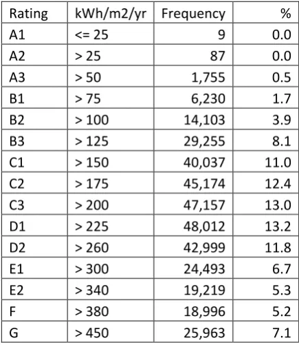
The Sustainable Energy Authority of Ireland (SEAI) is the agency responsible for BERs in Ireland and maintains a register of completed BERs.1 BERs are calculated by a standard assessment procedure, which models energy consumption under standard occupancy and normal climatic conditions, following European standards.2 A BER does not cover energy used for purposes other than those associated with heating and lighting (e.g. electricity used by kitchen appliances, etc., is not included). In Ireland a BER rating is reported as the total primary energy used and expressed in kilowatt hours per unit area per annum (kWh/m2/year), which is subsequently classified into a 15-point alpha-numeric scale (A1, A2,
…, E1, E2, F, G), details of which are in Table 1. A low kWh/m2/year indicates a good energy
performance with the alpha-numeric rating beginning with A1 for the most efficient down to G, the lowest energy performance. Actual BER ratings are based on the technical specifications of the property, including heating and ventilation equipment, and are calculated using a bespoke software and procedure.3 The median property in the BER database has a C3 BER rating, which is between 200-225 kWh/m2/year, though the database
is not necessarily representative of the total housing stock. The most frequent BER classifications are between C1 and D2.
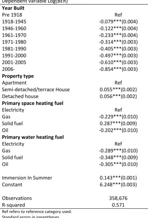
We use the BER database, which contains information on household characteristics, to develop a classification regression for BER ratings as a function of key predictor indicators. The key indicators are building age, and type (e.g. apartment), and the fuel used for space and water heating. In the classification regression we confine the explanatory variables to variables that are also contained in the household expenditure dataset, which is used in the next stage of analysis. The regression results are presented in Table 2, where the dependent variable is the logarithm of the BER rating. From this regression we find that recently built properties have progressively better BER ratings. This reflects both improvements in building practice, technologies, and building code regulations over time and mirrors a similar result for property in the UK (DCLG (2010)). An inherent flaw in the model in this case is that the model uses building age and ignores, due to lack of data, whether any refurbishment occurred subsequently. Semi-detached, terrace and detached houses generally have a poorer BER than apartments. The regression uses electricity as the reference fuel for both space and water heating. Properties that use gas or oil as the primary fuel, either for space or water heating, generally have better BER ratings than properties using electricity. We also find that properties that use solid fuel for water heating (e.g. a coal fuelled fireplace with
1 The database of BERs is available to download at
http://www.seai.ie/Your_Building/BER/National_BER_Research_Tool/
2 IS EN 13790: Energy performance of buildings - Calculation of energy use for space heating and cooling 3 Details of the assessment procedure and software are available at
integrated boiler) generally have a better BER rating than properties that primarily use electricity for water heating.
While the model only uses a few explanatory variables, it works reasonably well explaining actual BER ratings with a coefficient of determination, R2, of 0.57. The estimated model,
which relies on a relatively small sub-set of the technical data utilised in making an actual BER assessment, explains 57% of the total variation of outcomes. When comparing the actual BER rating with the model predicted BER (both in logarithms), the predicted log BER rating is within 5% of the actual log BER rating for 70% of observations (or within 25% of the BER in kWh/m2/year for 67% of observations). The model is poor at predicting properties
with high energy efficiency but across the entire BER dataset just 6% of properties were classified in the top 5 BER categories (A1 to B2). The model is better suited to predicting properties in the bottom ten BER categories. The most frequent BER classifications for Irish residential property are classes C1 to D2, accounting for 62% of properties assessed with a further 24% in classes E1 to G. The regression estimates in Table 2, which are based on the BER dataset, are used to predict a BER classification for each property associated with the households in the household expenditure dataset.
Estimating fuel expenditure equations
Ireland’s Central Statistics Office undertakes a Household Budget Survey (HBS) of a representative random sample of all private households in the State with the primary purpose of determining the pattern of household expenditure to update the weighting basis of the Consumer Price Index. During the survey households are required to maintain a detailed diary of household expenditure over a two-week period, including fuel expenditure. Details of bulk fuel purchases during the year outside the two-week diary period are also elicited. The survey was most recently undertaken between August 2009 and September 2010 with 5,891 household participants (CSO (2012)).
Using the HBS dataset we estimate fuel expenditure equations as a function of BER rating and other household characteristics. Expenditure equations, or Engel curves, are often estimated to investigate how expenditure on a particular good varies with household income. Many studies have investigated the best specification for the form of the Engel curves; Prais and Houthakker (1955) and Leser (1963) are notable examples. The ‘Leser-Working’ form of Engel curve in which budget shares are regressed on the log of income or expenditure has been widely used in empirical applications. The Almost Ideal Demand System (AIDS) specification of Deaton and Muellbauer (1980b) is an example, whereas alternative specifications have also included quadratic or inverse terms for expenditure or income, such as in Pollak and Wales (1980). Using earlier HBS survey data for Ireland both Leser (1964) and more recently Conniffe (2000a) estimated Engel functions, with actual expenditure on fuel 𝑖 rather than fuel share as the dependent variable as a function of income, 𝑌.
To incorporate household characteristics (H) and the effect of properties’ BER on fuel expenditure we assume that they have an impact on the constant term, such that
𝒆𝒊= 𝛂𝒊+ 𝛄𝒊𝐥𝐧(𝐁𝐄𝐑) + 𝛗𝒊𝐇 + 𝜷𝒊𝒍𝒏(𝒀) (2)
From this we can derive two elasticities of interest. The fuel expenditure elasticity of income,
ξ𝑒𝑖Y, is the percentage change in expenditure on fuel 𝑖 for a percentage change in income.
The fuel expenditure elasticity of BER rating, ξ𝑒𝑖BER, is the percentage change in expenditure
on fuel 𝑖 for a percentage change in BER value.
𝛏𝒆𝒊𝐘= 𝛃𝒊
𝒆𝒊 (3)
𝛏𝒆𝒊𝐁𝐄𝐑= 𝛄𝒊
𝒆𝒊 (4)
Estimating (2) for total fuel expenditure is straightforward and from a policy perspective potentially of most interest for investigating whether relating to household fuel poverty or energy efficiency. Estimation of fuel specific expenditure equations is slightly more complex. With the exception of electricity, all households do not purchase each fuel type. In the case of gas, oil and solid fuels there are numerous observations with zero expenditure. Data censoring of this nature is a frequently encountered problem in applied demand analysis (e.g. Long (1997); Deaton and Muellbauer (1980a) Yen and Lin (2006)) and disregarding censoring produces biased estimates. Tobin (1958) was the first to address the issue and develop a modified approach to analysing consumer demand. Numerous models have subsequently been developed to address the censoring issue, including the Heckman selection model (Heckman (1979); Heckman (1976); Lewis (1976); Gronau (1974)). The Heckman approach is formulated as a two equation model, a detailed explanation of which can be found in Greene (2002). The first equation determines selection into the sample, in this case it is the qualitative decision whether to purchase a fuel or not, and takes the following form:
𝐳𝒊∗= 𝜹𝒊𝐃 + 𝛎 (5)
The second equation describes the quantitative decision, in this case how much fuel to purchase
𝒆𝒊= 𝛂𝒊+ 𝛄𝒊𝐥𝐧(𝐁𝐄𝐑) + 𝛗𝒊𝐇 + 𝜷𝒊𝒍𝒏(𝒀) + 𝛆 = 𝚽𝒊𝐗 + 𝛆 (6)
Where 𝑒𝑖 is observed if z𝑖∗ is greater than zero, i.e.:
𝒆𝒊= � 𝚽𝒊𝐗 + 𝛆 𝑖𝑓 𝒛𝒊 ∗> 𝟎
− 𝑖𝑓 𝒛𝒊∗= 𝟎 (7)
The error terms, 𝜈 and ε are assumed bivariate normal with correlation coefficient 𝜌:
𝒄𝒐𝒓𝒓(𝛎, 𝛆) = 𝝆
We suspect that the error terms are correlated (i.e. that 𝜌 ≠ 0). For instance, how much fuel a household purchases depends on whether such a fuel is either available to or convenient for a particular household. Mains gas connection is limited to the major urban areas where the gas network exists. Bottled gas or other fuels are widely available but a household’s energy infrastructure (i.e. whether it can accommodate every available fuel) or the type of energy using equipment within a household will affect which fuels a household will seek to purchase. Consequently we estimate using the Heckman procedure.
We model the decision to purchase a fuel as a function of household characteristics. It is not unreasonable to assume that properties built in certain locations, during certain periods or properties of specific types may be more likely to use one fuel over another: e.g. oil in rural areas, gas in urban areas, or electricity in apartments. While the decision on whether to purchase a fuel may also be a function of the availability of the fuel locally, the HBS dataset does not contain information of this nature so cannot be incorporated into the estimated selection equation.
Data
explanatory variable in the expenditure equation potentially biases coefficient estimates. We investigate this issue using bootstrap techniques.
Results
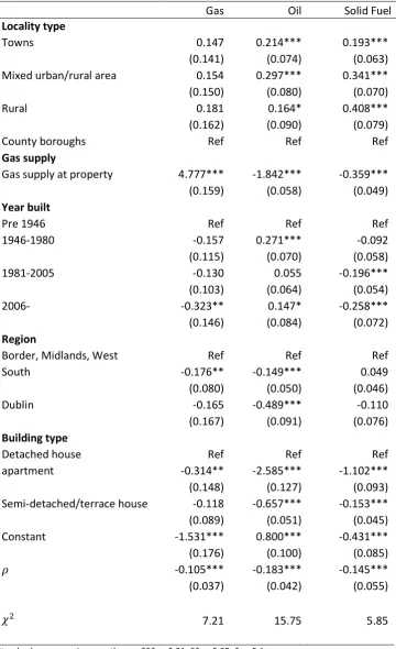
The gas, oil and solid fuel expenditure equations were estimated with the ‘heckman’ routine within Stata, which jointly estimates the selection and expenditure equations by maximum likelihood. The results for the selection equations are reported in Table 4. The 𝜒2 statistic
reported for each equation is a likelihood ratio test equivalent to 𝜌 = 0, that the Heckman selection equation is appropriate.
The variables that are statistically important in the selection equations vary by fuel but access or connectivity to fuel appears to be important. Mains gas connectivity is an important factor in explaining the decision to purchase gas, though there is always the option of bottled gas. Both the region and locality variables possibly capture some element of fuel availability in terms of access to the gas network or the conventional fuel choice in certain localities. Building type is also important because building types preclude certain fuel choices. For example, many apartments were built when gas supply was not permitted by building regulations nor is oil storage convenient so these fuels are significantly less likely to be purchased by apartment dwellers.
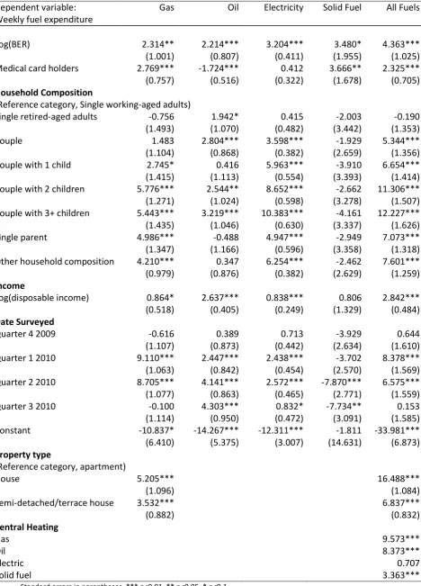
The Engel equation estimates are presented in Table 5. The gas, oil and solid fuel equations are estimated by the Heckman procedure, equation (7), whereas the electricity and total fuel expenditure equations are estimated by OLS. As might be anticipated fuel expenditure is affected by household composition. In general, households with children spend more on fuels than the reference category of a single working-aged adult. This is reflects the fact that proportionately more families compared to single adults live in larger properties that generally require more heating and with more people require more hot water. In the case of solid fuel we find no discernible affect of family composition on expenditure.
The ‘medical card holders’ variable is a dummy for households that are recipients of a means-tested health care support that is used as a proxy for other social welfare supports, including a fuel allowance. The parameter estimates suggest that such households spend more on fuel, except oil, compared to non-medical card recipients.
Whereas Nesbakken (1999) estimates income elasticities between 0.18-0.22 for energy among Norwegian households.
The primary focus of this paper is the coefficient estimate on the BER variable. Across all fuels the coefficient is statistically significant. Improved energy efficiency, as calculated by BER ratings, is associated with lower levels of household energy expenditure. The BER ratings are measures of kWh/m2/year so a positive sign was expected; higher BER ratings are
associated with higher levels of fuel expenditure. The BER elasticities of fuel expenditure, calculated at mean fuel expenditure per equation (6), are reported in Table 7. The elasticity estimates are relatively low in magnitude ranging from 0.18 to 0.32 for gas, oil and electricity but substantially higher at 1.08 for solid fuels. The BER elasticity estimate for all fuel expenditure is estimated at 0.12. We had no clear a priori on the size of these elasticities, nor are aware of comparative estimates elsewhere.
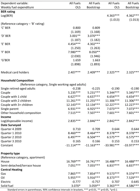
Assuming a single BER elasticity value for all types of properties and in particular for properties across the BER spectrum is restrictive and probably unrealistic. One might expect that the proportionate change in energy expenditure associated with a change in energy efficiency would be greater in properties with poor energy efficiency. We re-estimated the models using a discrete BER variable based on the 7 letter categories in the BER. The estimates for the total energy expenditure equation are presented in Table 8. The re-estimated fuel specific equations are not reported as the individual coefficient estimates on the discrete BER variables were generally not statistically significant. The BER reference category used in the regression is a B BER rating so the coefficients are interpreted relative to energy expenditure in B rated properties. All coefficients are positive so properties with poorer energy efficiency ratings spend more on energy, controlling for other factors. Properties with an E rating spend on average €4.45 per week more on energy than B rated properties, whereas households in F rated properties spend €7.98 more per week. At a 5% significance level the C and G coefficients are insignificantly different than B rated properties. Given that B and C ratings are adjacent we would expect that difference in energy expenditure to be lowest across BER categories. But finding the coefficient for the most energy inefficient properties, i.e. G rated, to be insignificant (and the magnitude of the coefficient to be relatively low) was unexpected and is difficult to explain. Properties with G ratings are a disparate group and have a disproportionate representation of low income households, and households in the “other household composition” category that was described in Table 3.
estimates for the G rated properties aside, these estimates suggest that a one letter change in BER rating is associated with expenditure changes of 4-10%.
As noted earlier the inclusion of an estimated BER value as an explanatory variable may potentially lead to bias in coefficient estimates. To address this issue the “all fuel” expenditure equation was re-estimated (both the continuous and discrete BER variable cases) using a bootstrap technique. Using the mean and variance-covariance estimates associated with the classification regression (Table 2), which was used to estimate a BER rating for households in the HBS survey, and assuming a normal distribution 100,000 draws of the parameter vector were generated. For each draw an estimated BER rating was calculated for each of the 5,812 households in the HBS dataset and an expenditure equation for total fuel expenditure was re-estimated. The bootstrap estimates are also presented in Table 8, where we find that there is no substantial difference in the coefficients compared to the original OLS estimates. Households in D rated properties spend €3.07 per week more on energy; €4.30 in E rated properties; €8.07 in F rated properties compared to B rated properties. The parameter estimate on G rated properties is not statistically significant (i.e. not different than B rated properties). Over the course of a year households in D, E and F rated properties spend €160, €224 and €419 more on energy per annum than households in B rated properties.
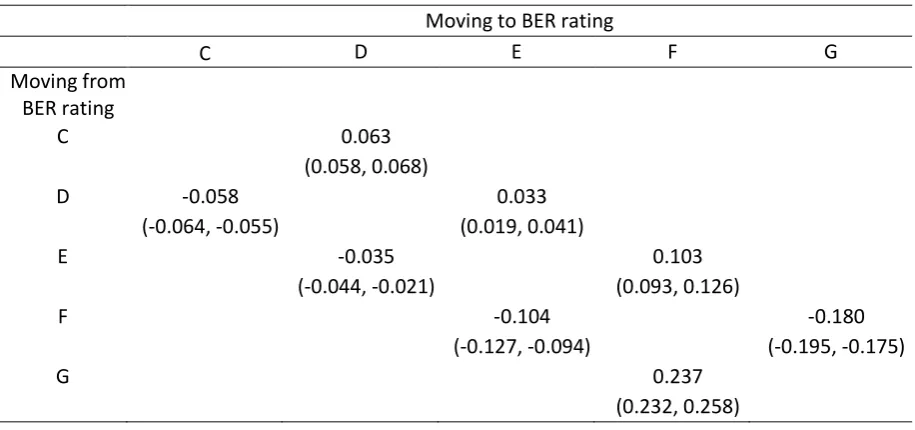
Table 10 reports the associated BER elasticities, including 90% confidence intervals, from the bootstrap estimation. Only elasticities that are significantly different than zero are reported in Table 10, and are consistent with the earlier reported elasticities. There is roughly a 6% difference in energy expenditure associated with C and D rated properties; a 4% difference associated with D and E properties; and a 10% difference associated with E and F properties. The BER elasticity associated with a continuous BER rating variable calculated from the bootstrap analysis is 0.121 with a 90% confidence interval of (0.120, 0.122). This is a point elasticity estimate and is comparable in magnitude to the previous estimate. As noted earlier it is somewhat unrealistic to expect a constant elasticity value across properties with substantially different levels of energy efficiency.
These elasticity estimates are not measures of cause and effect for a number of reasons. The expenditure dataset is a cross-section panel and while households will differ across the panel, the data is not measuring a response to a change in building energy efficiency. Second, there may be other unobserved factors correlated with a property’s BER rating that affect energy consumption, for example, daytime occupancy rates and associated space heating requirements.
one letter improvement along the BER scale (e.g. D to C) is associated with approximately a 6-14% reduction in energy expenditure for lighting, heating and ventilation purposes. Improvements in energy efficiency are also widely coupled with rebound effects, where the energy efficiency improvements are offset by increased energy consumption. There is considerable debate in the literature on the magnitude of the rebound with estimates varying by sector and region. In a review of some 500 rebound studies Sorrell (2007) concludes that the direct rebound effect for household heating is likely to be less than 30%. On that basis a one letter change in BER value (e.g. D to C) might be associated with a potential 8.5-20% reduction in energy expenditure for lighting, heating and ventilation purposes assuming no change in behaviour or rebound effect.
The authors were unable to find a directly comparable analysis in the literature but it is interesting to compare with a study by Scheer et al. (2013), which examines the direct effect on energy consumption due to investment in energy efficiency investments in a sample of 210 Irish households. Their analysis finds that investments in energy efficiency retro-fits achieved a 17–24% reduction in energy use. Their analysis focuses on energy use rather than expenditure. The proportionate change in energy use is necessarily greater than energy expenditure due to the fixed tariff element of utility bills but even allowing for this it is likely that elasticity estimates here are likely to be lower than the unknown expenditure reductions in Scheer et al’s study. However, it should be noted that the Scheer et al. analysis specifically examined energy savings associated with property retrofits using ex ante and ex post data (from a sample that is potentially prone to selection bias), whereas the analysis here is based on cross-section panel data that did not measure household responses to changes in building energy efficiency.
Hyland et al. (2013) examine the effect of Irish BER ratings on house prices and rental rates. When prices were analysed by BER letter scale the rental premium for a one letter change in BER rating (e.g. C to D or vice versa) ranged between 1.3-4.5%, whereas in property sales the price premium varied between 1.7-11%. Property buyers and renters recognise the value of better BER ratings (presumably capitalising the value of energy expenditure savings in higher rental or sales prices). It is not possible to directly compare the results of both analyses the magnitude of these price premiums is not inconsistent with the BER elasticity estimates above.
Conclusions
relationship between BER and energy expenditure we must analyse energy expenditure data. Investigating the relationship between building energy costs and energy efficiency ratings is difficult, as information about building energy performance, energy consumption and household occupancy are not usually recorded together or easily matched. The approach here uses the BER dataset to model BER ratings as a function of household characteristics, which is then analysed in the context of household occupancy and energy consumption.
The analysis finds statistical support for the assertion that improvements in energy efficiency, as calculated by BER ratings, is associated with reductions in household energy expenditure. For all energy expenditure the point estimate of the BER elasticity is 0.12 but we find that the elasticity varies depending on the energy efficiency of properties. We find that a one letter change in BER rating between C and F ratings is associated with a 4-10% change in total energy expenditure, or approximately 6-14% change in energy expenditure for heating, lighting and ventilation purposes (i.e. BER-related energy). Over the course of a year households in D, E and F rated properties spend €160, €224 and €419 more on energy per annum than households in B rated properties. For the most energy efficient properties we did not detect a statistically significant change in energy expenditure associated with a one letter change in BER rating (e.g. from a C to B rated property). For the least energy efficient properties (i.e. G rated) we found results contrary to expectations: an improvement in energy efficiency is associated with higher energy expenditure. This result is most likely a reflection of the data employed rather than a representation of reality. The data used is a cross-section household panel and captures variation across households rather than within household responses to changes in building energy efficiency. A second issue is that in the dataset the most and least energy efficient properties represent just 7% and 8% respectively of the observations in the dataset and the result may be driven by sample size.
Table 1: BER classification for residential buildings in Ireland
Rating kWh/m2/yr Frequency %
A1 <= 25 9 0.0
A2 > 25 87 0.0
A3 > 50 1,755 0.5
B1 > 75 6,230 1.7
B2 > 100 14,103 3.9
B3 > 125 29,255 8.1
C1 > 150 40,037 11.0
C2 > 175 45,174 12.4
C3 > 200 47,157 13.0
D1 > 225 48,012 13.2
D2 > 260 42,999 11.8
E1 > 300 24,493 6.7
E2 > 340 19,219 5.3
F > 380 18,996 5.2
G > 450 25,963 7.1
Table 2: Classification regression for BER for residential buildings
Dependent variable Log(BER) Year Built
Pre 1918 Ref
1918-1945 -0.079***(0.004)
1946-1960 -0.122***(0.004)
1961-1970 -0.233***(0.004)
1971-1980 -0.314***(0.003)
1981-1990 -0.405***(0.003)
1991-2000 -0.497***(0.003)
2001-2005 -0.610***(0.003)
2006- -0.854***(0.003)
Property type
Apartment Ref
Semi-detached/terrace House 0.055***(0.002)
Detached house 0.056***(0.002)
Primary space heating fuel
Electricity Ref
Gas -0.229***(0.010)
Solid fuel 0.287***(0.009)
Oil -0.202***(0.010)
Primary water heating fuel
Electricity Ref
Gas -0.289***(0.010)
Solid fuel -0.348***(0.009)
Oil -0.305***(0.010)
Immersion In Summer 0.143***(0.001)
Constant 6.248***(0.003)
Observations 358,676
R-squared 0.571
Table 3: Descriptive Statistics, Household Budget Survey
Variable Obs Mean Std. Dev. Min Max
Electricity expenditure (€/week) 5872 17.44 10.25 0 126.98
Gas expenditure(€/week) 5872 8.62 14.39 0 304.70
Oil expenditure (€/week) 5872 6.92 11.01 0 162.25
Solid fuel expenditure (€/week) 5872 3.21 13.91 0 750.00
Total energy expenditure (€/week) 5872 36.19 23.61 1.91 765.10
BER - kWh/m2/year 5872 265.99 103.14 97.73 840.06
Log (BER) 5872 5.52 0.35 4.58 6.73
Medical card holders 5872 0.39 0.49 0 1
Single working-aged adults 5872 0.15 0.36 0 1
Single retired-aged adults 5872 0.07 0.26 0 1
Couple 5872 0.17 0.37 0 1
Couple 1 child 5872 0.07 0.25 0 1
Couple 2 children 5872 0.09 0.28 0 1
Couple 3 or more children 5872 0.07 0.26 0 1
Single adult 5872 0.07 0.26 0 1
Other household composition 5872 0.30 0.46 0 1
Disposable income (€/week) 5872 905.37 671.30 0.38 12341.93
Log disposable income (€/week) 5872 6.57 0.73 -0.97 9.42
Urban/Rural
County bourghs & suburbs 5872 0.39 0.49 0 1
Towns 5872 0.29 0.45 0 1
Mixed urban/rural area 5872 0.19 0.39 0 1
Rural 5872 0.12 0.33 0 1
Gas/Electricity connection
Electricity only 5872 0.57 0.50 0 1
Both Electricity and gas 5872 0.43 0.50 0 1
Year property built
pre 1945 5872 0.17 0.37 0 1
1946-1980 5872 0.26 0.44 0 1
1981-2005 5872 0.44 0.50 0 1
2006- 5872 0.13 0.34 0 1
Region
Border, Midland and West 5872 0.27 0.44 0 1
South 5872 0.43 0.49 0 1
Dublin 5872 0.31 0.46 0 1
Property type
Apartment 5872 0.14 0.35 0 1
Semi-detached /terrace house 5872 0.52 0.50 0 1
Table 4: Heckman selection equation estimates
Gas Oil Solid Fuel
Locality type
Towns 0.147 0.214*** 0.193***
(0.141) (0.074) (0.063)
Mixed urban/rural area 0.154 0.297*** 0.341***
(0.150) (0.080) (0.070)
Rural 0.181 0.164* 0.408***
(0.162) (0.090) (0.079)
County boroughs Ref Ref Ref
Gas supply
Gas supply at property 4.777*** -1.842*** -0.359*** (0.159) (0.058) (0.049) Year built
Pre 1946 Ref Ref Ref
1946-1980 -0.157 0.271*** -0.092
(0.115) (0.070) (0.058)
1981-2005 -0.130 0.055 -0.196***
(0.103) (0.064) (0.054)
2006- -0.323** 0.147* -0.258***
(0.146) (0.084) (0.072) Region
Border, Midlands, West Ref Ref Ref
South -0.176** -0.149*** 0.049
(0.080) (0.050) (0.046)
Dublin -0.165 -0.489*** -0.110
(0.167) (0.091) (0.076) Building type
Detached house Ref Ref Ref
apartment -0.314** -2.585*** -1.102***
(0.148) (0.127) (0.093) Semi-detached/terrace house -0.118 -0.657*** -0.153*** (0.089) (0.051) (0.045)
Constant -1.531*** 0.800*** -0.431***
(0.176) (0.100) (0.085)
𝜌 -0.105*** -0.183*** -0.145***
(0.037) (0.042) (0.055)
𝜒2 7.21 15.75 5.85
Table 5: Fuel expenditure equation regressions
Dependent variable:
Weekly fuel expenditure Gas Oil Electricity Solid Fuel All Fuels
Log(BER) 2.314** 2.214*** 3.204*** 3.480* 4.363***
(1.001) (0.807) (0.411) (1.955) (1.025) Medical card holders 2.769*** -1.724*** 0.412 3.666** 2.325*** (0.757) (0.516) (0.322) (1.678) (0.705) Household Composition
(Reference category, Single working-aged adults)
Single retired-aged adults -0.756 1.942* 0.415 -2.003 -0.190
(1.493) (1.070) (0.482) (3.442) (1.353)
Couple 1.483 2.804*** 3.598*** -1.929 5.344***
(1.104) (0.868) (0.382) (2.659) (1.356)
Couple with 1 child 2.745* 0.416 5.963*** -3.910 6.654***
(1.415) (1.113) (0.554) (3.393) (1.414) Couple with 2 children 5.776*** 2.544** 8.652*** -2.662 11.306*** (1.271) (1.024) (0.598) (3.278) (1.507) Couple with 3+ children 5.443*** 3.219*** 10.383*** -4.161 12.227*** (1.435) (1.046) (0.630) (3.337) (1.626)
Single parent 4.986*** -0.488 4.947*** -2.949 7.073***
(1.347) (1.166) (0.596) (3.358) (1.318) Other household composition 4.210*** 0.347 6.254*** -2.462 7.601*** (0.979) (0.876) (0.382) (2.629) (1.259) Income
Log(disposable income) 0.864* 2.637*** 0.838*** 0.806 2.842*** (0.518) (0.405) (0.249) (1.329) (0.484) Date Surveyed
Quarter 4 2009 -0.616 0.389 0.713 -3.929 0.644
(1.107) (0.873) (0.442) (2.634) (1.610)
Quarter 1 2010 9.110*** 2.447*** 2.438*** -3.702 8.378***
(1.063) (0.842) (0.454) (2.570) (1.569)
Quarter 2 2010 8.705*** 4.141*** 2.572*** -7.870*** 6.575***
(1.077) (0.863) (0.465) (2.771) (1.559)
Quarter 3 2010 -0.100 4.303*** 0.832* -7.734** 0.153
(1.114) (0.950) (0.472) (3.091) (1.585)
Constant -10.837* -14.267*** -12.311*** -1.811 -33.981***
(6.410) (5.375) (3.007) (14.631) (6.873) Property type
(Reference category, apartment)
House 5.205*** 16.488***
(1.096) (1.084)
Semi-detached/terrace house 3.532*** 6.837***
(0.882) (0.832)
Central Heating
Gas 9.573***
Oil 8.373***
Electric 0.707
Solid fuel 3.363***
Table 6: Income elasticity estimates, including estimates from previous Household Budget Surveys
HBS 1951-52 1965-66 1973 1980 1987 1994-95 2004-05 2009-10 Total fuels 0.5 0.32 0.46 0.48 0.43 0.25 0.22 0.08***
Gas 0.48 0.47 0.2 0.44 0.37 0.75 0.39 0.10*
Electricity 1.01 0.82 0.87 0.72 0.76 0.35 0.35 0.05*** Coal 0.59 0.08 ns 0.06 ns 0.02 ns -0.01 ns -0.29 ns -0.33 0.25nsa
Turf na 0.51 -0.69 -0.55 -0.5 -0.3 na na
Oil na na na 1.54 1.85 0.96 0.27 0.38***
Source: Leser (1964); Pratschke (1969); Murphy (1976); Conniffe and Scott (1990); Conniffe (2000a); Scott et al. (2008). na: no estimate available. ns: estimate not statistically significant. a The estimate for 2009-10 relates to solid fuels and not specifically coal. *** p<0.01, ** p<0.05, * p<0.1.
Table 7: BER elasticities of fuel expenditure
Gas Oil Electricity Solid
Fuel All fuels BER elasticity 0.27** 0.32*** 0.18*** 1.08* 0.12***
(0.12) (0.12) (0.02) (0.61) (0.03)
[image:19.595.90.428.361.452.2]
Table 8: Fuel expenditure equation regressions
Dependent variable:
Weekly fuel expenditure All Fuels OLS Bootstrap All Fuels All Fuels OLS Bootstrap All Fuels BER rating
Log(BER) 4.363*** 4.362***
(1.013) (1.013) (Reference category – ‘B’ rating)
‘C’ BER 0.800 0.809
(1.169) (1.168)
‘D’ BER 3.001** 3.070***
(1.187) (1.182)
‘E’ BER 4.454*** 4.302***
(1.250) (1.263)
‘F’ BER 7.980*** 8.050**
(2.030) (1.946)
‘G’BER 1.659 1.663
(1.898) (1.893)
Medical card holders 2.407*** 2.409*** 2.325*** 2.325***
Household Composition
(Reference category, Single working-aged adults)
Single retired-aged adults -0.238 -0.225 -0.190 -0.190
Couple 5.235*** 5.231*** 5.344*** 5.345***
Couple with 1 child 6.627*** 6.637*** 6.654*** 6.654***
Couple with 2 children 11.261*** 11.255*** 11.306*** 11.306*** Couple with 3+ children 12.143*** 12.134*** 12.227*** 12.227***
Single parent 6.931*** 6.925*** 7.073*** 7.073***
Other household composition 7.515*** 7.507*** 7.601*** 7.601*** Income
Log(disposable income) 2.835*** 2.846*** 2.842*** 2.842***
Date Surveyed
Quarter 4 2009 0.710 0.709 0.644 0.644
Quarter 1 2010 8.460*** 8.464*** 8.378*** 8.378***
Quarter 2 2010 6.497*** 6.504*** 6.575*** 6.575***
Quarter 3 2010 0.165 0.166 0.153 0.153
Constant -11.114*** -11.163*** -33.981*** -33.977***
Property type
(Reference category, apartment)
House 16.769*** 16.741*** 16.488*** 16.488***
Semi-detached/terrace house 7.051*** 7.055*** 6.837*** 6.837*** Central Heating
Gas 7.865*** 7.854*** 9.573*** 9.374***
Oil 5.955*** 5.916*** 8.373*** 7.529***
Electric -0.777 -0.757 0.707 0.645
Solid fuel 3.070* 3.059** 3.363*** 4.586***
Table 9: Discrete BER expenditure elasticities
Moving to BER rating Avg. weekly
energy
expenditure B C D E F G
Moving from BER rating
B 34.38 0.023
C 36.29 -0.022 0.061***
D 38.53 -0.057*** 0.038*
E 35.65 -0.041* 0.099**
F 35.35 -0.100** -0.179***
G 26.73 0.236***
[image:21.595.90.548.340.555.2]*** p<0.01, ** p<0.05, * p<0.1
Table 10: Discrete BER expenditure elasticities and 90% confidence intervals
Moving to BER rating
C D E F G
Moving from BER rating
C 0.063
(0.058, 0.068)
D -0.058 0.033
(-0.064, -0.055) (0.019, 0.041)
E -0.035 0.103
(-0.044, -0.021) (0.093, 0.126)
F -0.104 -0.180
(-0.127, -0.094) (-0.195, -0.175)
G 0.237
Bibliography
Australian Bureau of Statistics. 2008. Energy efficiency rating and house price in the ACT, Department of the Environment, Water, Heritage and the Arts, Canberra.
Berkhout, P. H. G., Muskens, J. C., and Velthuijsen, W. 2000. "Defining the rebound effect", Energy Policy, vol. 28, no. 6-7, pp. 425-432.
Brounen, D. and Kok, N. 2011. "On the economics of energy labels in the housing market", Journal of Environmental Economics and Management, vol. 62, no. 2, pp. 166-179.
Cajias, M. and Piazolo, D. 2013. "Green performs better: energy efficiency and financial return on buildings", Journal of Corporate Real Estate, vol. 15, no. 1, pp. 53-72.
CEC. 2011. Energy Efficiency Plan 2011, Communication from the Commission to the European Parliament, the Council, the European Economic and Social Committee and the Committee of the Regions, COM(2011) 109.
Chakravarty, D., Dasgupta, S., and Roy, J. 2013. "Rebound effect: How much to worry?", Current Opinion in Environmental Sustainability, vol. 5, no. 2, pp. 216-228.
Conniffe, D. 2000a. Household Energy Expenditures: Policy Relevant Information from the Household Budget Survey, Policy Research Series, 37. ESRI, Dublin.
Conniffe, D. 2000b. "The Free Electricity Allowance and the Engel Curve", The Economic and Social Review, vol. Vol. 31, No. 2, April 2000, pp. 173-186.
Conniffe, D. and Scott, S. 1990. Energy Elasticities: Responsiveness of Demands for Fuels to Income and Price Changes, General Research Series, 149. ESRI, Dublin.
CSO. 2012. Household Budget Survey 2009-2010, Central Statistics Office, Dublin. DCLG. 2010. English Housing Survey: Housing stock report 2008, Department for Communities and Local Government (DCLG), London.
Deaton, A. and Muellbauer, J. 1980a, Economics and Consumer Behavior.
Deaton, A. and Muellbauer, J. 1980b. "An Almost Ideal Demand System", American Economic Review, vol. 70, 312-326.
Dennehy, E. and Howley, M. 2013. Energy in the Residential Sector 2013 Report, Sustainable Energy Authority of Ireland.
Eichholtz, P., Kok, N., and Quigley, J. M. 2010. "Doing Well by Doing Good? Green Office Buildings", American Economic Review, vol. 100, no. 5, 2492-2509.
EP and CEC. 2002. Directive 2002/91/EC on the Energy Performance of Buildings, Directive 2002/91/EC of the European Parliament and of the Council of 16 December 2002 on the energy performance of buildings.
Greene, W. H. 2002, Econometric Analysis. 5th edn, Prentice Hall, New Jersey.
Gronau, R. 1974. "Wage comparisons: A selectivity bias", Journal of Political Economy, vol. 82, no. 6, pp. 1119-1143.
Heckman, J. J. 1976. "The common structure of statistical models of truncation, sample selection and limited dependent variables and a simple estimator for such models", Annals of Economic and Social Measurement, vol. 5, pp. 475-492.
Heckman, J. J. 1979. "Sample Selection Bias as a Specification Error", Econometrica, vol. 47, no. 1, 153-161.
Herring, H. 2006. "Energy efficiency - A critical view", Energy, vol. 31, no. 1 SPEC. ISS., pp. 10-20.
Hyland, M., Lyons, R. C., and Lyons, S. 2013. "The value of domestic building energy efficiency - evidence from Ireland", Energy Economics, vol. 40, pp. 943-952.
Jamasb, T. and Meier, H., 2010. "Household Energy Expenditure and Income Groups: Evidence from Great Britain" Cambridge Working Paper in Economics 1101
Kok, N. and Jennen, M. 2012. "The impact of energy labels and accessibility on office rents", Energy Policy, vol. 46, no. 0, pp. 489-497.
Leser, C. E. V. 1963. "Forms of Engel Functions", Econometrica, vol. Vol. 31, No. 4, October 1963.
Leser, C. E. V. 1964. A Further Analysis of Irish Household Budget Data, 1951-1952, General Research Series, 23. ESRI, Dublin.
Lewis, H. G. 1976. "Comments on Selectivity Biases in Wage Comparisons", Journal of Political Economy, vol. 82, no. 6, pp. 1145-1155.
Long, J. S. 1997, Regression Models for Categorical and Limited Dependent Variables. Sage, Thousand Oaks.
Meier, H., Jamasb, T., and Orea, L., 2012. "Necessity or Luxury Good? Household Energy Spending and Income in Britain 1991-2007" Cambridge Working Paper in Economics 1239 Murphy, D. C. 1976. "1973 Household Budget Survey: special features and results", Journal of the Statistical and Social Inquiry Society of Ireland, vol. XXIII, no. III, pp. 135-191.
Nässén, J. and Holmberg, J. 2009. "Quantifying the rebound effects of energy efficiency improvements and energy conserving behaviour in Sweden", Energy Efficiency, vol. 2, no. 3, pp. 221-231.
Nesbakken, R. 1999. "Price sensitivity of residential energy consumption in Norway", Energy Economics, vol. 21, no. 6, pp. 493-515.
Pollak, R. A. and Wales, T. J. 1980. "Comparison of the Quadratic Expenditure System and Translog Demand Systems with Alternative Specifications of Demographic Effects", Econometrica, vol. 49, 595-612.
Prais, S. J. and Houthakker, H. S. 1955, The Analysis of Family Budgets. Cambridge University Press.
Pratschke, J. L. 1969. Income-Expenditure Relations in Ireland, 1965-1966, General Research Series, 50. ESRI, Dublin.
Reichardt, A., Fuerst, F., Rottke, N. B., and Zietz, J. 2012. "Sustainable Building Certification and the Rent Premium: A Panel Data Approach", Journal of Real Estate Research, vol. 34, no. 1, 99-126.
Scheer, J., Clancy, M., and Ní Hógáin, S. 2013. "Quantification of energy savings from Ireland's Home Energy Saving scheme: an ex post billing analysis", Energy Efficiency, vol. 6, no. 1, pp. 35-48.
Scott, S., Lyons, S., Keane, C., McCarthy, D., and Tol, R. S. J., 2008. "Fuel Poverty in Ireland: Extent, Affected Groups and Policy Issues", ESRI Working Paper 262, ESRI, Dublin.
SEAI. 2013. Dwelling Energy Assessment Procedure: Introduction to DEAP for Professionals, Sustainable Energy Authority of Ireland.
Sorrell, S., Dimitropoulos, J., and Sommerville, M. 2009. "Empirical estimates of the direct rebound effect: A review", Energy Policy, vol. 37, no. 4, pp. 1356-1371.
Sorrell, S. 2007. The Rebound Effect: an assessment of the evidence for economy-wide energy savings from improved energy efficiency, UK Energy Research Centre (UK ERC).
Thomson, H. and Snell, C. 2013. "Quantifying the prevalence of fuel poverty across the European Union", Energy Policy, vol. 52, no. 0, pp. 563-572.
Tobin, J. 1958. "Estimation of Relationships for Limited Dependent Variables", Econometrica, vol. 26, no. 1, pp. 24-36.
Year Number
Title/Author(s)
ESRI Authors/Co-authors Italicised
2014
477 A Computational Theory of Willingness to Exchange Pete Lunn and Mary Lunn
476 Who Feels Inferior? A Test of the Status Anxiety Hypothesis of Social Inequalities in Health
Richard Layte and Christopher T. Whelan
2013
475 Factor Input Substitution in Irish Manufacturing Stefanie A. Haller and Marie Hyland
474 Changes in Income Distributions and the Role of Tax-benefit Policy During the Great Recession: An International Perspective
Olivier Bargain, Tim Callan, Karina Doorley and Claire Keane 473 International Migration in Ireland, 2012
Philip J. O’Connell and Corona Joyce
472 Does Bank Market Power Affect SME Financing Constraints? Robert M. Ryan, Conor M. O’Toole, Fergal McCann
471 Consumption and credit constraints: A model and evidence for Ireland Petra Gerlach-Kristen and Rossana Merola
470 Socioeconomic Differentials in Male Mortality in Ireland: 1984-2008 Richard Layte and Anne Nolan
469 Deriving a Method to Estimate Incidence of Stroke in Ireland Maev-Ann Wren and Peter Kelly
468 The Impact of Parental Income and Education on the Schooling of Children Arnaud Chevalier, Colm Harmon, Vincent O’Sullivan, Ian Walker
467 SME Credit Constraints and Macroeconomic Effects Petra Gerlach-Kristen, Brian O’Connell and Conor O’Toole
466 Transitions In and Out of Unemployment Among Young People in the Irish Recession
Elish Kelly, Seamus McGuinness, Philip O’Connell, David Haugh and Alberto González Pandiella
For earlier Working Papers see