Sources into the Semantic Web
?Craig A. Knoblock1, Pedro Szekely1, Jose Luis Ambite1, Aman Goel1, Shubham Gupta1, Kristina Lerman1, Maria Muslea1, Mohsen Taheriyan1, and
Parag Mallick2
1
University of Southern California
Information Sciences Institute and Department of Computer Science {knoblock,pszekely,ambite,amangoel,shubhamg,lerman,mariam,mohsen}@isi.edu
2
Stanford University Department of Radiology
Abstract. Linked data continues to grow at a rapid rate, but a limita-tion of a lot of the data that is being published is the lack of a semantic description. There are tools, such as D2R, that allow a user to quickly convert a database into RDF, but these tools do not provide a way to easily map the data into an existing ontology. This paper presents a semi-automatic approach to map structured sources to ontologies in order to build semantic descriptions (source models). Since the precise mapping is sometimes ambiguous, we also provide a graphical user interface that allows a user to interactively refine the models. The resulting source mod-els can then be used to convert data into RDF with respect to a given ontology or to define a SPARQL end point that can be queried with respect to an ontology. We evaluated the overall approach on a variety of sources and show that it can be used to quickly build source models with minimal user interaction.
1
Introduction
The set of sources in the Linked Data cloud continues to grow rapidly. Many of these sources are published directly from existing databases using tools such as D2R [8], which makes it easy to convert relational databases into RDF. This con-version process uses the structure of the data as it is organized in the database, which may not be the most useful structure of the information in RDF. But either way, there is often no explicit semantic description of the contents of a
?
This research is based upon work supported in part by the Intelligence Advanced Research Projects Activity (IARPA) via Air Force Research Laboratory (AFRL) contract number FA8650-10-C-7058. The views and conclusions contained herein are those of the authors and should not be interpreted as necessarily representing the official policies or endorsements, either expressed or implied, of IARPA, AFRL, or the U.S. Government.
source and it requires a significant effort if one wants to do more than simply convert a database into RDF. The result of the ease with which one can publish data into the Linked Data cloud is that there is lots of data published in RDF and remarkably little in the way of semantic descriptions of much of this data.
In this paper, we present an approach to semi-automatically building source models that define the contents of a data source in terms of a given ontology. The idea behind our approach is to bring the semantics into the conversion process so that the process of converting a data source produces a source model. This model can then be used to generate RDF triples that are linked to an ontology and to provide a SPARQL end point that converts the data on the fly into RDF with respect to a given ontology. Users can define their own ontology or bring in an existing ontology that may already have been used to describe other related data sources. The advantage of this approach is that it allows the source to be transformed in the process of creating the RDF triples, which makes it possible to generate RDF triples with respect to a specific domain ontology.
The conversion to RDF is a critical step in publishing sources into the Linked Data cloud and this work makes it possible to convert sources into RDF with the underlying semantics made explicit. There are other systems, such as R2R [7] and W3C’s R2RML [9], that define languages for specifying mappings between sources, but none of this work provides support for defining these mappings. This paper describes work that is part of our larger effort on developing techniques for performing data-integration tasks by example [23]. The integrated system is available as an open-source tool called Karma3.
2
Motivating Example
The bioinformatics community has produced a growing collection of databases with vast amounts of data about diseases, drugs, proteins, genes, etc. Nomen-clatures and terminologies proliferate and significant efforts have been under-taken to integrate these sources. One example is the Semantic MediaWiki Linked Data Extension (SMW-LDE) [5], designed to support unified querying, naviga-tion, and visualization through a large collection of neurogenomics-relevant data sources. This effort focused on integrating information from the Allen Brain At-las (ABA) with standard neuroscience data sources. Their goal was to “bring ABA, Uniprot, KEGG Pathway, PharmGKB and Linking Open Drug Data [16] data sets together in order to solve the challenge of finding drugs that target elements within a disease pathway, but are not yet used to treat the disease.”
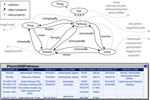
We use the same scenario to illustrate and evaluate our contributions, com-paring our results to the published SMW-LDE results (see Figure 1). We use logical rules to formally define the mapping between data sources and an ontol-ogy. Specifically, we use global-local-as-view (GLAV) rules [13] commonly used in data integration [15] and data exchange [3] (i.e., rules whose antecedent and consequent are conjunctive formulas). The rule antecedent is the source relation
3
keggDrugId name alternativeSymbolalternativeLabel pharmGKBId keggGeneId keggDiseaseId keggPathwayId description abaGeneId entrezGeneId uniprotId geneSymbol Pathway Top Thing Drug Gene Disease : subclass : object property : data property causes disrupts involves isCausedBy isDisruptedBy isInvolvedIn isTargetedBy isTreatedBy treats targets
PharmGKBPathways(Accession Id, Name, Drug Id, Drug Name, Gene Id, Gene Name, Disease Id, Disease Name)→
Pathway(uri(Accession Id)) ˆname(uri(Pathway Id),Name) ˆ
involves(uri(Pathway Id),uri(Gene Id)) ˆ
isTargetedBy(uri(Pathway Id),uri(Drug Id)) ˆ
isDisruptedBy(uri(Pathway Id),uri(Disease Id)) ˆ
Gene(uri(Gene Id)) ˆgeneSymbol(uri(Gene Id),Gene Name) ˆ Drug(uri(Drug Id)) ˆname(uri(Drug Id),Drug Name) ˆ Disease(uri(Disease Id)) ˆname(uri(Disease Id),Disease Name)
Fig. 1.The ontology used in the SMW-LDE study, one of the KEGG Pathway sources used, and the source model that defines the mapping of this source to the ontology. that defines the columns in the data source. The rule consequent specifies how the source data elements are defined using the ontology terms. For example, the first term,Pathway(uri(Accession Id))specifies that the values in the Acces-sion Id column are mapped to thePathwayclass, and that these values should
be used to construct the URIs when the source description is used to gener-ate RDF. The second term,name(uri(Accession Id),Name)specifies that the values in theAccession Idare related to the values in theNamecolumn using thename property.
The task in the SMW-LDE scenario is to define source models for 10 data sources. Writing these source models by hand, or the equivalent R2R rules is laborious and requires significant expertise. In the next sections we describe how our system can generate source models automatically and how it enables users to intervene to resolve ambiguities.
Learned Semantic Types KARMA Assign Semantic Types Construct Graph GUI Refine Source Model Generate Formal
Specification SourceModel customize
override
Source Ontology
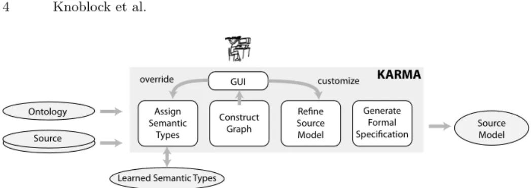
Fig. 2.The Karma process to model structured sources.
3
Modeling Structured Sources
Figure 2 illustrates our approach for modeling data sources. The inputs to the process are an OWL ontology, the collection of data sources that the user wants to map to the ontology, and a database of semantic types that the system has learned to recognize based on prior use of the tool. The main output is the model that specifies, for each source, the mapping between the source and the ontology. A secondary output is a refined database of semantic types, updated during the process to incorporate semantic types learned using the data contained in the sources being mapped.
As shown in Figure 2, the modeling process consists of four main steps. The first step,Assign Semantic Types, involves mapping each column of a source to a node in the ontology. This is a user-guided process where the system assigns types automatically based on the data values in each column and a set of learned probabilistic models constructed from assignments done in prior sessions. If the semantic type assigned by the system is incorrect, the user can select from a menu the correct node in the graph. The system learns from this assignment and records the learned assignment in its database. The second step,Construct Graph, involves constructing a graph that defines the space of all possible map-pings between the source and the ontology. At a high level, the nodes in the graph represent classes in the ontology, and the edges represent properties that relate these classes. The mapping from the ontology to the graph is not one-to-one given that, for example, several columns may contain instances of the same class (Section 3.2). The third step, Refine Source Model, updates the graph to refine the model based on user input. The graph is constructed so that the map-ping between the source and the ontology can be computed using a Steiner tree algorithm (Section 3.3). The final fourth step, Generate Formal Specification, generates a formal specification of the source model from the Steiner tree com-puted in the prior step (Section 3.5). An example of this formal specification appears in the bottom part of Figure 1.
In general, it is not always possible to automatically compute the desired mapping between a source and an ontology since there may not be enough in-formation in the source to determine the mapping. So, the automated process
computes the most succinct mapping, and the user interface allows the user to guide the process towards the desired interpretation (Section 3.4).
3.1 Inferring the Semantic Types
Semantic typescharacterize the type of data that appears in a column of data. For example, in the table shown in Figure 1, the first column contains Phar-mGKB identifiers of pathways, the second one contains names of pathways, etc. In some cases, semantic types correspond to classes in an OWL ontology, but in most cases, they could be most naturally thought of as the ranges of data properties. It is possible to define semantically meaningful RDFS types in OWL and use them as the ranges of data properties. However, few ontologies define such types. The ranges of data properties are almost always missing, or they are defined using syntactic types such as String or Integer.
In our modeling framework, a semantic type can be either an OWL class or a pair consisting of a data property and an OWL class (the property domain or a subclass of it). We use OWL classes to define the semantic types of columns of data that contain automatically-generated database keys or foreign keys (dur-ing RDF generation, these keys are used to generate URIs). We use semantic types defined in terms of data properties and their domain for columns con-taining meaningful data. In our example, the first column contains PharmGKB identifiers of pathways, so the values can be characterized by the semantic type consisting of the data property pharmGKBId and the class Pathway, or Path-way.pharmGKBIdfor short.
Karma provides a user interface to let users assign semantic types to the columns of a data source. In this section we present our approach for automating the assignment of semantic types by learning from prior assignments defined in the user interface. The objective is to learn a labeling functionφ(n,{v1, v2, . . .}) =
tso that givenn, the name of a column, and{v1, v2, . . .}, the values in that col-umn, it assigns a semantic typet∈T, whereT is the set of semantic types used during training. The training data consists of a set of prior assignments of seman-tic typestito columns of data:{(n1,{v11, v12, . . .}, t1),(n2,{v21, v22, . . .}, t2), . . .}.
We use a conditional random field (CRF) [18] to learn the labeling function. Before giving the details of how we build the feature vectors to train the CRF, we first explain how we define φ in terms of a function ˆφthat we use to label individual values in a column of data. Given a column name n and a single value v in that column, ˆφ(n, v) = {(v, tk, pk), tk ∈ T} gives for each tk in T
the probabilitypk that the semantic type ofv istk. To label a column of data
(n,{v1, v2, . . .}), we compute ˆφ(n, vi) for each value vi ∈ {v1, v2, . . .}, and then compute the average probability over all values in a column. The result is a set of pairs ¯φ(n,{v1, v2, . . .}) = {(t1, p1),(t2, p2), . . .}. Based on this set, we define
φ(n,{v1, v2, . . .}) =tm, the type with maximum probability, i.e.,tmis such that
(tm, pm) ∈ φ¯(n,{v1, v2, . . .}) and pm ≥ pi for all (tk, pk) ∈ φ¯(n,{v1, v2, . . .}). When users load a source, Karma automatically labels every column using
The task is now to learn the labeling function ˆφ(n, v). As mentioned above, users label columns of data, but to learn ˆφ(n, v) we need training data that assigns semantic types to each value in a column. We assume that columns contain homogeneous values, so from a single labeled column (n,{v1, v2, . . .}, t) we generate a set of training examples {(n, v1, t),(n, v2, t), . . .} as if each value in the column had been labeled using the same semantic typet.
For each triple (n, v, t) we compute a feature vector (fi) that characterizes
the syntactic structure of the column name nand the valuev. To compute the feature vector, we first tokenize the name and the value. Our tokenizer uses white space and symbol characters to break strings into tokens, but identifies numbers as single tokens. For example, the name Accession Id produces the tokens (“Accession”, “ ”, “Id”), the value PA2039 produces the tokens (“PA”, 2039), and the value72.5◦Fproduces the tokens (72.5,◦,F).
Eachfi is a Boolean feature functionfi(n, v) that tests whether the name,
value or the resulting tokens have a particular feature. For example, valueS-tartsWithA,valueStartsWithB,valueStartsWithPAare three different feature func-tions that test whether the value starts with the characters ‘A’, ‘B’or the sub-string“PA”;hasNumericTokenWithOrderOfMagnitude1, hasNumericTokenWithOr-derOfMagnitude10are feature functions that test whether the value contains nu-meric tokens of order of magnitude 1 and 10 respectively. In general, features are defined using templates of the form predicate(X), and are instantiated for different values of X that occur within the training data. In our scenario, valueS-tartsWith(X)is instantiated with X=‘P’ and X=‘A’because “PA2039” is in the first column and “Arthritis, Rheumatiod” is in the last column; however, there will be no valueStartsWithB feature because no value starts with the character ‘B’. Our system uses 21 predicates; the most commonly instantiated ones are:
nameContainsToken(X), nameStartsWith(X), valueContainsToken(X), valueStarts-With(X), valueHasCapitalizedToken(), valueHasAllUppercaseToken(), valueHasAl-phabeticalTokenOfLength(X), valueHasNumericTokenWithOrderOfMagnitude(X), valueHasNumericTokenWithPrecision(X), valueHasNegativeNumericToken().
A CRF is a discriminative model, and it is practical to construct feature vectors with hundreds or even thousands of overlapping features. The model learns the weight for each feature based on how relevant it is in identifying the semantic types by optimizing a log-linear objective function that represents the joint likelihood of the training examples. A CRF model is useful for this problem because it can handle large numbers of features, learn from a small number of examples, and exploit the sequential nature of many structured formats, such as dates, temperatures, addresses, etc. To control execution times, our system labels and learns the labeling function using at most 100 randomly selected values from a column. With 100 items, labeling is instantaneous and learning takes up to 10 seconds for sources with over 50 semantic types.
3.2 Constructing the Graph
The central data structure to support the mapping of sources to the ontology is a graph computed from the semantic types of the source and the domain
ACCESSION_ID GENE_ID DRUG_ID NAME GENE_NAME DRUG_NAME DISEASE_NAME DISEASE_ID Pathway1 Top1 Drug1 Gene1 Disease1
: Edp : Eop : Esc
: Vtp
: Voc, Vtc # : weight Xxx : column name
pharmGKBId1 pharmGKBId4 pharmGKBId2 pharmGKBId3 name1 geneSymbol1 name3 name2 1/ε 1/ε 1/ε 1/ε 1 1 1 1 1 1 1 1 1 1 1 1 1 1 1 1 1 1
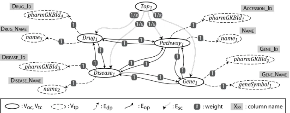
Fig. 3.The graph defines the search space for source models and provides the infor-mation for the user interface to enable users to refine the computed source model. ontology. The algorithm for building the graph has three sequential steps: graph initialization, computing nodes closure, and adding the links.
Graph Initialization: We start with an empty graph called G. In this step, for each semantic type assigned to a column, a new node with a unique label is added to the graph. A semantic type is either a class in the ontol-ogy or a pair consisting of the name of a datatype property and its domain. We call the corresponding nodes in the graph Vtc and Vtp respectively.
Apply-ing this step on the source shown in Figure 3 results in Vtc = {} and Vtp =
{pharmGKBId1, pharmGKBId2, pharmGKBId3, pharmGKBId4, name1,
name2,name3,geneSymbol1}.
Computing Nodes Closure: In addition to the nodes that are mapped from semantic types, we have to find nodes in the ontology that relate those semantic types. We search the ontology graph and for every class node that has a path to the nodes corresponding to semantic types, we create a node in the graph. In other words, we get all the class nodes in the ontology from which the semantic types are reachable. To compute the paths, we consider both properties andisarelationships. The nodes added in this step are calledVoc. In the example,
we would haveVoc ={T hing1,T op1,Gene1, P athway1, Drug1, Disease1}. In Figure 3, solid ovals represent {Vtc∪Voc}, which are the nodes mapped from
classes of ontology, and the dashed ovals represent Vtp, which are the semantic
types corresponding to datatype properties.
Adding the Links:The final step in constructing the graph is adding the links to express the relationships among the nodes. We connect two nodes in the graph if there is a datatype property, object property, or isarelationship that connects their corresponding nodes in the ontology. More precisely, for each pair of nodes in the graph,uandv:
– Ifv∈Vtp, i.e.,vis a semantic type mapped from a datatype property, and
u corresponds to the domain class of that semantic type, we create a directed weighted link (u, v) with a weight equal to one (w = 1). For example, there would be a link from P athway1 to pharmGKBId1, because pharmGKBId1 corresponds to the semantic typePathway.pharmGKBId.
– Ifu, v∈ {Vtc∪Voc}, which means both of them are mapped from ontology
classes, we put a weighted link (u, v) with w = 1 in the graph only if there is an object property such as p in the ontology whose domain includes the class of uand whose range includes class of v. These links are calledEop. Note that
the properties inherited from parents are also considered in this part, but to prioritize direct properties in the algorithm, we consider a slightly higher weight to the inherited properties. In other words, if pis defined such that its domain contains one of the superclasses ofu(at any level) and its range contains one of the superclasses ofv, we add the link (u, v) withw= 1 +.
– Ifu, v∈ {Vtc∪Voc}andvis a direct or indirect subclass ofu, a link (u, v)
with w = 1/ is added to the graph, in which is a very small value. We call these linksEsc. Subclass links have a large weight so that relationships mapped
from properties are preferred over the relationships through the class hierarchy. The final graph is a directed weighted graph G = (V, E) in which V = {Vtp∪Vtc∪Voc}and E={Edp∪Eop∪Esc}. Figure 3 shows the final graph. 3.3 Generating Source Models
Source models must explicitly represent the relationships between the columns of a source. For example, after mapping columns to theGeneand Drugclasses, we want to explicitly represent the relationship between these two classes. The graph we constructed in the previous section explicitly represents all possible relationships among the semantic types. We construct a source model as the minimal tree that connects the semantic types The minimal tree corresponds to the most succinct model that relates all the columns in a source, and this is a good starting point for refining the model. To compute the minimal tree, we use one of the variations of the known Steiner Tree algorithm. Given an edge-weighted graph and a subset of the vertices, called Steiner nodes, the goal is to find the minimum-weight tree in the graph that spans all Steiner nodes. In our graph, the Steiner nodes are the semantic type nodes, i.e., the set {Vtc∪Vtp}.
The Steiner tree problem is NP-complete, but we use a heuristic algorithm [17] with an approximation ratio bounded by 2(1−1/l), where l is the number of leaves in the optimal Steiner tree. The time complexity of the algorithm is
O(|Vtc∪Vtp||V|2). Figure 4(a) shows the resulting Steiner tree.
It is possible that multiple minimal trees exist, or that the correct interpreta-tion of the data is specified by a non-minimal tree. In these cases, Karma allows the user to interactively impose constraints on the algorithms that lead to the correct model. We enforce these constraints onGby transforming it into a new graph G0, and usingG0 as the input to the Steiner tree algorithm. User actions
can have three types of effects on the algorithm:
Changing the semantic types:If the user changes the semantic type of one or more columns, we re-construct the graph G and repeat all the steps mentioned before to get the final Steiner tree.
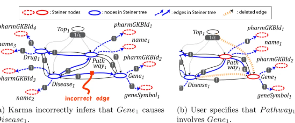
Specifying a relationship:In the Steiner tree shown in Figure 4(a),Disease is related to Gene through the isCausedBy property. However, in the correct model of the data, Gene is related to Pathway through the involves property.
: edges in Steiner tree : deleted edge : nodes in Steiner tree
: Steiner nodes incorrect edge pharmGKBId1 pharmGKBId4 pharmGKBId2 pharmGKBId3 name1 geneSymbol1 name3 name2 Path way1 Top1 Drug1 Gene1 Disease1 1/ε 1 1 1 1 1 1 1 1 1 1 1 1 1
(a) Karma incorrectly infers that Gene1 causes Disease1. pharmGKBId1 pharmGKBId2 name1 geneSymbol1 Pathway 1 Top1 Gene1 Disease1 1/ε 1 1 1 1 1 1 1 1 1 ε
(b) User specifies that P athway1
involvesGene1.
Fig. 4.Interactive refinement of the automatically computed Steiner trees. Karma allows the user to correct the model and change the relationship from
isCausedBy to involves. To force the Steiner tree algorithm to select the new link, we first add the source (P athway1) and target (Gene1) of the link to the Steiner nodes. Then we remove all the incoming links to the target except the link selected by the user. This means thatinvolves would be the only link in the graph going toGene1. Finally, we reduce the weight of the user link to. These steps guarantee that the user link will be chosen by the Steiner algorithm. Note that forcing a link by the user does not change graphG and it only affectsG0
and the Steiner nodes. Figure 4(b) illustrates the new G0 and Steiner tree after selecting the involves relationship by the user.
Generating multiple instances of a class:Consider the case that in the source table, in addition to information about the genes involved in pathway, we also have the data about genes that cause specific diseases. This means that, for example, we have two columnsGene Name1andGene Name2referring to different genes. Suppose that the CRF model has assigned theGene.geneSymbol semantic type to both columns and their corresponding nodes in the graph are
geneSymbol1 and geneSymbol2. After constructing the graph, we would have
two outgoing links from Gene1 to geneSymbol1 and geneSymbol2, indicating that Gene Name1andGene Name2are different symbols of the sameGene. However, the correct model is the one in whichGene Name1andGene Name2
are symbols for two different genes. That is, there should be two instances of theGeneclass,Gene1andGene2that are separately connected togeneSymbol1
andgeneSymbol2. To solve this problem, Karma gives the option to the user to
generate multiple instances of a class in the GUI. The user selects the Gene1 node and splits it based on the geneSymbolproperty. ThenG0 and the Steiner tree are re-computed to produce the correct model.
3.4 User Interface for Refining Semantic Models
Karma visualizes a source model as a tree of nodes displayed above the column headings of a source. Figure 5 shows the visualization of the source model corre-sponding to the Steiner tree shown in Figure 4(a). The root of the Steiner tree
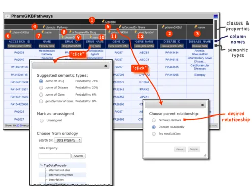
desired relationship column names classes & properties semantic types “click” “click” 1 4 5 7 8 9 10 11 12 2 3 6
Fig. 5.Karma screen showing the PharmGKBPathways source. Clicking on the pencil icon brings up a menu where users can specify alternative relationships between classes. Clicking on a semantic type brings up a menu where the user can select the semantic types from the ontology. A movie showing the user interface in action is available at http://isi.edu/integration/videos/karma-source-modeling.mp4.
appears at the top, and shows the name of the class of objects that the table is about (in our example the table is about diseases4). The Steiner nodes corre-sponding to the semantic types are shown just below the column headings. The nodes between the root and the semantic types show the relationships between the different objects represented in the table. Internal nodes of the Steiner tree (e.g., nodes 4, 5 and 8) consist of the name of an object property, shown in italics and a class name (a subclass of the range of the property). The property defines the relationship between the class named in the parent node and the class of the current node. For example, node 4 is “disruptsPathway”, which means that the Disease (node 1) disrupts the Pathway represented by the columns under node 4. The leaves of the tree (nodes 6, 7, 9, etc.) show the name of data prop-erties. For example, node 6 ispharmGKBId, meaning that the column contains thepharmGKBId of thePathwayin node 4.
According to the model shown in Figure 5, the table contains information about diseases (1): the last column contains the disease names (3) and the next to last column contains their identifiers (2). TheDiseasedisruptsa Pathway(4), and isCausedBy a Gene(5). ThePathway is identified using itspharmGKBId in
4 Selection of the root is not unique for ontologies that declare property inverses.
In this example, any of the classes could have been selected as the root yielding equivalent models.
1 4
5
Fig. 6.Karma screen showing the user interaction to change the model of a column from a Pathway label to a Drug label.
the first column (6), and itsnameappears in the second column (7). ThePathway
isTargeted by theDrug(8) whose identifier (9) and label (10) appear in the third and fourth columns. The gene that causes the disease (5) is identified using its
pharmGKBId (11) and itsgeneSymbol (12).
This is a plausible model, but it is incorrect because the table lists the genes involved in the pathways that are disrupted by the disease instead of the genes that cause the disease; in other words, theisCausedByproperty in cell 5 is incor-rect. Users can edit the model to adjust the relationships between columns by clicking on the pencil icons. The pop-up in Figure 5 appears the user clicks on the pencil icon on theGenecell (5): it shows the possible relationships corresponding to all incoming edges to theGene1node in the graph shown in Figure 3. Figure 6 shows the adjusted model after the user selects the “Pathway Involves” option in Figure 5 to specify the correct relationship between the disease and the gene. TheGenecell (5) is now belowPathway(4) related using theinvolves property. Karma also provides capabilities to clean, normalize and transform data be-fore modeling it. For example, a source in our scenario contained alternative symbols for genes as comma-separated values stored in individual cells (e.g., “CP12, P3-450, P450(PA)”). Karma provides a “split cell” command to break the value into multiple cells so that each value can be modeled as a separate al-ternative symbol. These commands can be saved in scripts to enable automatic preprocessing of sources when source models are used to generate RDF.
3.5 Generation of Formal Source Model Specification
After users have (optionally) imposed constraints to reflect the correct seman-tics, the system processes the resulting Steiner tree to generate GLAV rules that provide a formal specification of (1) how the sources are combined and which at-tributes of the source are relevant, (2) how the source data maps to the ontology, and (3) how URIs for objects in the ontology are generated. We illustrate the algorithm that generates the GLAV rule of Figure 1 based on the Steiner tree from Figure 4(b), which corresponds to the user interface shown in Figure 6.
Class nodesgenerate unary predicates corresponding to classes in the on-tology. The urifunction builds URIs for class instances based on the key(s), or foreign key(s), in the source tables. For example, thePathwaynode in Figures 3 and 6 generates the predicatePathway(uri(Accession Id)) because the values in theAccession Idcolumn represent instances of Pathway.
The system also supports class nodes that are not associated with a source column. These correspond to existentially quantified variables in the rule con-sequent and would generate blank nodes in RDF. However, we generate unique regular URIs to support linking (owl:sameAs) into these URIs at a later stage. For example, assume that the ontology included a Mutation class, where a Gene has a Mutation that causes a Disease, then the corresponding fragment of the rule consequent would be:hasMutation(uri(Gene Id),uri(1)) ˆ Mutation(uri(1)) ˆ causes(uri(1),uri(Disease Id)). The index in theuri function is used to iden-tify different existentially quantified variables.
Data property nodes generate binary predicates corresponding to data properties in the ontology. For example, thename1node associated withPathway in Figure 3 generates the binary predicate name(uri(Accession Id), Name), specifying that instances of Pathway have the name data property filled with values from theNamecolumn.
Edgesbetween class nodes generate binary predicates corresponding to ob-ject properties in the ontology. For example, the edge between Pathway1 and Gene1 in Figure 4(b) generates the predicateinvolves(uri(Accession Id),
uri(Gene ID)).
The resulting GLAV rules can now be used to generate the appropriate RDF for a source in terms of the domain ontology, as in data exchange [3]. Alterna-tively, the mappings can be interpreted dynamically by a mediator, as in data integration [15]. The mediator would provide a SPARQL endpoint exposing the ontology and executing queries directly over the original sources.
4
Evaluation
We evaluated our approach by generating source models for the same set of sources integrated by Becker et al.[5], as described in Section 2. The objective of the evaluation was 1) to assess the ability of our approach to produce source models equivalent to the mappings Becker et al. defined for these sources, and 2) to measure the effort required in our approach to create the source models. Becker et al. defined the mappings using R2R, so we used their R2R mapping files as a specification of how data was to be mapped to the ontology. Our objective was to replicate the effect of the 41 R2R mapping rules defined in these files. Each R2R mapping rule maps a column in our tabular representation. We measured effort in Karma by counting the number of user actions (number of menu choices to select correct semantic types or adjust paths in the graph) that the user had to perform. Effort measures for the R2R solution are not available, but appears to be substantial given that the rules are expressed in multiple pages of RDF.
Using Karma we constructed 10 source models that specify mappings equiv-alent to all of the 41 R2R mapping rules. Table 1 shows the number of actions required to map all the data sources. The Assign Semantic Type column shows the number of times we had to manually assign a semantic type. We started this evaluation with no training data for the semantic type identification. Out of the 29 manual assignments, 24 were for specifying semantic types that the system had never seen before, and 5 to fix incorrectly inferred types.
Table 1.Evaluation Results for Mapping the Data Sources using Karma. Source Table Name # Columns # User Actions
Assign Semantic Type Specify Relationship Total
PharmGKB Genes 8 8 0 8 Drugs 3 3 0 3 Diseases 4 4 0 4 Pathways 5 2 1 3 ABA Genes 6 3 0 3 Drugs 2 2 0 2 KEGG Diseases 2 2 0 2 Pathway Genes 1 1 0 1 Pathways 6 3 1 4 UniProt Genes 4 1 0 1
Total: 41 Total: 29 Total: 2 Total: 31 Avg. # User Actions/Column = 31/41 = 0.76 Events database 19 Tables Total: 64 Total: 43 Total: 4 Total: 47
Avg. # User Actions/Column = 47/64 = 0.73 The Specify Relationship column shows the number of times we had to select alternative relationships using a menu (see Figure 5). For the PharmGKB and KEGG Pathway sources, 1 action was required to produce a model semantically equivalent to the R2R mapping rule. The total number of user actions was 31, 0.76 per R2R mapping rule, a small effort compared to writing R2R mapping rules in RDF. The process took 11 minutes of interaction with Karma for a user familiar with the sources and the ontology.
In a second evaluation, we mapped a large database of events into the ACE OWL Ontology [12]. The ontology has 127 classes, 74 object properties, 68 data properties and 122 subclass axioms. The database contains 19 tables with a total of 64 columns. We performed this evaluation with no training data for the semantic type identification. All 43 manual semantic type assignments were for types that the system had not seen before, and Karma was able to accurately infer the semantic types for the 21 remaining columns. Karma automatically computed the correct source model for 15 of 19 tables and required one manual relationship adjustment for each of the remaining 4 tables. The average number of nodes in our graph data structure was 108, less than the number of nodes in the ontology (127 classes and 68 types for data properties). The average time for graph construction and Steiner tree computation across the 19 tables was 0.82 seconds, which suggests that the approach scales to real mid-size ontologies. The process took 18 minutes of interaction with Karma.
5
Related Work
There is significant work on schema and ontology matching and mapping [21, 6]. An excellent recent survey [22] focuses specifically on mapping relational databases into the semantic web. Matching discovery tools, such as LSD [10] or COMA [20], produce element-to-element matches based on schemas and/or data. Mapping generation tools, such as Clio [11] and its extensions [2], Altova MapForce (altova.com), or NEON’s ODEMapster [4], produce complex map-pings based on correspondences manually specified by the user in a graphical interface or produced by matching tools. Most of these tools are geared toward expert users (ontology engineers or DB administrators). In contrast, Karma fo-cuses on enabling domain experts to model sources by automating the process
as much as possible and providing users an intuitive user interface to resolve ambiguities and tailor the process. Karma produces complex GLAV mappings under the hood, but users do not need to be aware of the logical complexities of data integration/exchange. They see the source data in a familiar spreadsheet format annotated with hierarchical headings, and they can interact with it to correct and refine the mappings.
Alexe et al. [1] elicit complex data exchange rules from examples of source data tuples and the corresponding tuples over the target schema. Karma could use this approach to explain its model to users via examples, and as an alternative method for users to customize the model by editing the examples.
Schema matching techniques have also been used to identify the semantic types of columns by comparing them with labeled columns [10]. Another ap-proach [19] is to learn regular expression-like rules for data in each column and use these expressions to recognize new examples. Our CRF approach [14] im-proves over these approaches by better handling variations in formats and by exploiting a much wider range of features to distinguish between semantic types that are very similar, such as those involving numeric values.
The combination of the D2R [8] and R2R [7] systems can also express GLAV mappings as Karma. D2R maps a relational database into RDF with a schema closely resembling the database. Then R2R can transform the D2R-produced RDF into a target RDF that conforms to a given ontology using an expressive transformation language. R2RML [9] directly maps a relational database to the desired target RDF. In both cases, the user has to manually write the mapping rules. In contrast, Karma automatically proposes a mapping and lets the user correct/refine the mapping interactively. Karma could easily export its GLAV rules into the R2RML or D2R/R2R formats.
6
Discussion
A critical challenge of the Linked Data cloud is understanding the semantics of the data that users are publishing to the cloud. Currently, users are linking their information at the entity level, but to provide deeper integration of the available data, we also need semantic descriptions in terms of shared ontologies. In this paper we presented a semi-automated approach to building the mappings from a source to a domain ontology.
Often sources require complex cleaning and transformation operations on the data as part of the mapping. We plan to extend Karma’s interface to express these operations and to include them in the source models. In addition, we plan to extend the approach to support modeling a source in which the relationships among columns contain a cycle.
References
1. Alexe, B., ten Cate, B., Kolaitis, P.G., Tan, W.C.: Designing and refining schema mappings via data examples. In: SIGMOD. pp. 133–144. Athens, Greece (2011)
2. An, Y., Borgida, A., Miller, R.J., Mylopoulos, J.: A semantic approach to dis-covering schema mapping expressions. In: Proceedings of the 23rd International Conference on Data Engineering (ICDE). pp. 206–215. Istanbul, Turkey (2007) 3. Arenas, M., Barcelo, P., Libkin, L., Murlak, F.: Relational and XML Data
Ex-change. Morgan & Claypool, San Rafael, CA (2010)
4. Barrasa-Rodriguez, J., G´omez-P´erez, A.: Upgrading relational legacy data to the semantic web. In: Proceedings of WWW Conference. pp. 1069–1070 (2006) 5. Becker, C., Bizer, C., Erdmann, M., Greaves, M.: Extending smw+ with a linked
data integration framework. In: Proceedings of ISWC (2010)
6. Bellahsene, Z., Bonifati, A., Rahm, E.: Schema Matching and Mapping. Springer, 1st edn. (2011)
7. Bizer, C., Schultz, A.: The R2R Framework: Publishing and Discovering Mappings on the Web. In: Proceedings of the First International Workshop on Consuming Linked Data (2010)
8. Bizer, C., Cyganiak, R.: D2R Server–publishing relational databases on the seman-tic web. In: Poster at the 5th International Semanseman-tic Web Conference (2006) 9. Das, S., Sundara, S., Cyganiak, R.: R2RML: RDB to RDF Mapping Language,
W3C Working Draft, 24 March 2011. http://www.w3.org/TR/r2rml/ (2011) 10. Doan, A., Domingos, P., Levy, A.Y.: Learning source descriptions for data
integra-tion. In: Proceedings of WebDB. pp. 81–86 (2000)
11. Fagin, R., Haas, L.M., Hernndez, M.A., Miller, R.J., Popa, L., Velegrakis, Y.: Clio: Schema mapping creation and data exchange. In: Conceptual Modeling: Founda-tions and ApplicaFounda-tions - Essays in Honor of John Mylopoulos. pp. 198–236 (2009) 12. Fink, C., Finin, T., Mayfield, J., Piatko, C.: Owl as a target for information
ex-traction systems (2008)
13. Friedman, M., Levy, A.Y., Millstein, T.D.: Navigational plans for data integration. In: Proceedings of AAAI. pp. 67–73 (1999)
14. Goel, A., Knoblock, C.A., Lerman, K.: Using conditional random fields to exploit token structure and labels for accurate semantic annotation. In: Proceedings of AAAI-11 (2011)
15. Halevy, A.Y.: Answering queries using views: A survey. The VLDB Journal 10(4), 270–294 (2001)
16. Jentzsch, A., Andersson, B., Hassanzadeh, O., Stephens, S., Bizer, C.: Enabling tailored therapeutics with linked data. In: Proceedings of the WWW Workshop on Linked Data on the Web (LDOW) (2009)
17. Kou, L., Markowsky, G., Berman, L.: A fast algorithm for steiner trees. Acta Informatica 15, 141–145 (1981)
18. Lafferty, J., McCallum, A., Pereira, F.: Conditional random fields: Probabilistic models for segmenting and labeling sequence data. In: Proceedings of the Eigh-teenth International Conference on Machine Learning. pp. 282–289 (2001) 19. Lerman, K., Plangrasopchok, A., Knoblock, C.A.: Semantic labeling of online
in-formation sources. IJSWIS, special issue on Ontology Matching (2006)
20. Massmann, S., Raunich, S., Aumueller, D., Arnold, P., Rahm, E.: Evolution of the coma match system. In: Proceedings of the Sixth International Workshop on Ontology Matching. Bonn, Germany (2011)
21. Shvaiko, P., Euzenat, J.: A survey of schema-based matching approaches. Journal on Data Semantics IV 3730, 146–171 (2005)
22. Spanos, D.E., Stavrou, P., Mitrou, N.: Bringing relational databases into the se-mantic web: A survey. Sese-mantic Web (2011), iOS Pre-press
23. Tuchinda, R., Knoblock, C.A., Szekely, P.: Building mashups by demonstration. ACM Transactions on the Web (TWEB) 5(3) (2011)