to Uncertain Volatility Models and CVA.
White Rose Research Online URL for this paper:
http://eprints.whiterose.ac.uk/99796/
Version: Published Version
Article:
Litterer, Christian, Ren, Zhenjie and Henry-Labordère, Pierre (2016) A dual algorithm for
stochastic control problems : Applications to Uncertain Volatility Models and CVA. SIAM
Journal on Financial Mathematics. pp. 159-182. ISSN 1945-497X
https://doi.org/10.1137/15M1019945
[email protected] https://eprints.whiterose.ac.uk/ Reuse
Items deposited in White Rose Research Online are protected by copyright, with all rights reserved unless indicated otherwise. They may be downloaded and/or printed for private study, or other acts as permitted by national copyright laws. The publisher or other rights holders may allow further reproduction and re-use of the full text version. This is indicated by the licence information on the White Rose Research Online record for the item.
Takedown
If you consider content in White Rose Research Online to be in breach of UK law, please notify us by
A Dual Algorithm for Stochastic Control Problems: Applications to Uncertain
Volatility Models and CVA
∗Pierre Henry-Labord`ere†, Christian Litterer‡, and Zhenjie Ren‡
Abstract. We derive an algorithm in the spirit of Rogers [SIAM J. Control Optim., 46 (2007), pp. 1116–1132] and Davis and Burstein [Stochastics Stochastics Rep., 40 (1992), pp. 203–256] that leads to upper bounds for stochastic control problems. Our bounds complement lower biased estimates recently obtained in Guyon and Henry-Labord`ere [J. Comput. Finance, 14 (2011), pp. 37–71]. We evaluate our estimates in numerical examples motivated by mathematical finance.
Key words. optimal stochastic control, duality theory, numerical methods
AMS subject classifications. 93E20, 49N15, 91G60
DOI. 10.1137/15M1019945
1. Introduction. Solving stochastic control problems, for example, by approximating the Hamilton–Jacobi–Bellman (HJB) equation, is an important problem in applied mathemat-ics. Classical PDE methods are effective tools for solving such equations in low-dimensional settings, but quickly become computationally intractable as the dimension of the problem increases: a phenomenon commonly referred to as “the curse of dimensionality.” Probabilistic methods on the other hand such as Monte Carlo simulation are less sensitive to the dimen-sion of the problem. It was demonstrated in Pardoux and Peng [16] and Cheridito et al. [3] that first and second backward stochastic differential equations (in short BSDE) can provide stochastic representations that may be regarded as a nonlinear generalization of the classical Feynman–Kac formula for semilinear and fully nonlinear second order parabolic PDEs.
The numerical implementation of such a BSDE-based scheme associated with a stochastic control problem was first proposed in Bouchard and Touzi [2], also independently in Zhang [19]. Further generalization was provided in Fahim, Touzi, and Warin [8] and in Guyon and Henry-Labord`ere [10]. The algorithm in [10] requires evaluating high-dimensional conditional expectations, which are typically computed using parametric regression techniques. Solving the BSDE yields a suboptimal estimation of the stochastic control. Performing an additional, independent (forward) Monte Carlo simulation using this suboptimal control, one obtains a biased estimation: a lower bound for the value of the underlying stochastic control problem. Choosing the right basis for the regression step is in practice a difficult task, particularly in high-dimensional settings. In fact, a similar situation arises for the familiar Longstaff–Schwarz
∗Received by the editors May 5, 2015; accepted for publication (in revised form) February 11, 2016; published
electronically April 19, 2016.
http://www.siam.org/journals/sifin/7/M101994.html
†Soci´et´e G´en´erale, Paris, France ([email protected]).
‡Centre de Math´ematiques Appliqu´ees, Ecole Polytechnique, Palaiseau, France ([email protected],
[email protected]). The second author’s research was supported by ERC grant 321111 RoFiRM. The third author’s research was supported by grants from R´egion Ile-de-France.
algorithm, which also requires the computation of conditional expectations with parametric regressions and produces a low-biased estimate.
As the algorithm in [10] provides a biased estimate, i.e., a lower bound, it is of limited use in practice, unless it can be combined with a dual method that leads to a corresponding upper bound. Such a dual expression was obtained by Rogers [17], building on earlier work by Davis and Burstein [4]. While the work of Rogers is in the discrete time setting, it applies to a general class of Markov processes. Previous work by Davis and Burstein [4] linking deterministic and stochastic control using flow decomposition techniques (see also Diehl, Friz, and Gassiat [5] for a rough path approach to this problem) is restricted to the control of a diffusion in its drift term. In the present paper we are also concerned with the control of diffusion processes, but allow the control to act on both the drift and the volatility term in the diffusion equation. The basic idea underlying the dual algorithm in all these works is to replace the stochastic control by a pathwise deterministic family of control problems that are not necessarily adapted. The resulting “gain” of information is compensated for by introducing a penalization analogous to a Lagrange multiplier. In contrast to [4] and [5], we do not consider continuous pathwise, i.e., deterministic, optimal control problems. Instead, we rely on a discretization result for the HJB equation due to Krylov [12] and recover the solution of the stochastic control problem as the limit of deterministic control problems over a finite set of discretized controls.
Our paper is structured as follows. In section 2 we introduce the stochastic control prob-lem and derive the dual bounds in the Markovian setting for European-type payoffs. In section 3.1we generalize our estimates to a non-Markovian setting, i.e., where the payoff has a path dependence. Finally, in section3.2we consider a setting suitable for pricing American style options in a Markov setting. We evaluate the quality of the upper bounds obtained in two numerical examples. First, we consider the pricing of a variety of options in the un-certain volatility model (UVM). Based on our earlier estimates we transform the stochastic optimization problem into a family of suitably discretized deterministic optimizations, which we can in turn approximate, for example, using local optimization algorithms. Second, we consider a problem arising in credit valuation adjustment. In this example, the deterministic optimization can particularly efficiently be solved by deriving a recursive ODE solution to the corresponding Hamilton–Jacobi equations. Our algorithm complements the lower bounds derived in [10] by effectively reusing some of the quantities already computed when obtaining the lower bounds (cf. Remark2.8).
2. Duality result for European options.
2.1. Notations. We begin by introducing some basic notations. For any k∈Nlet
Ωk :={ω :ω∈C([0, T],Rk), ω0 = 0}.
Let d, m ∈ N and T > 0. Define Ω := Ωd, Θ := [0, T]×Ω, and let B denote the canonical
process on Ωm with F={F
For h >0, consider a finite partition {th
i}i of [0, T] with mesh less than h, i.e., such that
thi+1−thi ≤h for all i. For someM >0, let Abe a compact subset of
OM :={x∈Rk:|x| ≤M} for some k∈N,
and Nh be a finite h-net of A, i.e., for all a, b∈Nh⊂A, we have|a−b| ≤h. We define sets
• A:={ϕ: Θ→Rk: ϕ isF-adapted, and takes values inA};
• Ah:={ϕ∈ A: ϕis constant on [tih, thi+1) fori, and takes values inNh}; • U :={ϕ: Θ→Rd: ϕis bounded andF-adapted};
• Dh :={f : [0, T]→Rk: f is constant on [thi, thi+1) for i, and takes values in Nh}. For the following it is important to note thatDh is a finite set of piecewise constant functions.
We would like to emphasize that, throughout this paper, C denotes a generic constant, which may change from line to line. For example the reader may find 2C ≤C, without any contradiction as the left-hand sideC is different from the right-hand sideC.
2.2. The Markovian case. We consider stochastic control problems of the form
(2.1) u0 = sup
α∈A
EP0
T
0
Rtαf(t, αt, Xtα)dt+RαTg(XTα)
,
whereRα t :=e−
t
0r(s,αs,Xsα)ds,Xα is ad-dimensional controlled diffusion defined by
Xα :=
·
0
µ(t, αt, Xtα)dt+ ·
0
σ(t, αt, Xtα)dBt,
and the functionsµ, σ, f, r satisfy the following assumption.
Assumption 2.1. The functions µ, σ, f, rdefined onR+×A×Rdtake values inRd,Rd×m, R,R, respectively. Assume that
• µ, σ, f, r are uniformly bounded, and continuous inα;
• µ, σ, f, r are uniformlyδ0-H¨older continuous int for some fixed constantδ0∈(0,1]; • µ, σ are uniformly Lipschitz in x, and f, r are uniformly δ0-H¨older continuous in x; • g:Rd→R is continuous.
Remark 2.2. Our assumptions match the assumptions on the continuity of the coefficients in Krylov [12,13], and allow us to apply his results.
Our main result is a duality in the spirit of [4] that allows us to replace the stochastic control problem by a family of suitably discretized deterministic control problems. We first discretize the control problem through the following lemma which is a direct consequence of Theorem 2.3 in Krylov [12].
Define the function
uh0 := sup
α∈Ah
EP0
T
0
Rαtf(t, αt, Xtα)dt+RαTg(XTα)
.
Lemma 2.3. Suppose Assumption 2.1 holds and g is bounded. We have for any family of partition of [0, T] with mesh tending to zero that
(2.2) u0 = lim
h→0u
h
Remark 2.4. Theorem 2.3 in [12] also gives a rate of convergence for the discretization in Lemma2.3, i.e., there exists a constant C >0 such that
u0−uh0
≤Ch13 for all 0< h≤1.
For the following statement, we introduce
(2.3)
vh := inf
ϕ∈U
EP0
max
a∈DhΦ
a,ϕ
with
Φa,ϕ:=RaTg(XTa) +
T
0
Ratf(t, at, Xta)dt− T
0
Ratϕt(Xa)⊺σ(t, at, Xta)dBt.
Remark 2.5. It is noteworthy that stochastic integrals are defined in L2-space, so it is in general meaningless to take the pathwise supremum of a family of stochastic integrals. However, as we mentioned before, the setDhis of finite elements. So there is a unique random
variable inL2 equal to the maximum value of the finite number of stochastic integrals, P0-a.s.
The next theorem allows us to recover the stochastic optimal control problem as a limit of discretized deterministic control problems.
Theorem 2.6. Suppose Assumption 2.1 holds andg is bounded. Then we have u0 = lim
h→0v
h.
Proof. We first prove that u0 ≤ limh→0vh. Recall uh0 defined in (2.2). Since Rα, σ are bounded, for allϕ∈ U the process0·Rα
tϕt(Xα)⊺σ(t, αt, Xtα)dBt is a martingale. So we have
uh0 = sup
α∈Ah
EP0Φα,ϕ.
Since Φα,ϕ≤max
a∈DhΦa,ϕ for all α∈ Ah, we have
uh0 ≤EP0
max
a∈DhΦ
a,ϕ
.
The required result follows.
To show u0 ≥ limh→0vh we construct an explicit minimizer ϕ∗. First note that under Assumption 2.1, it is easy to verify that utdefined as
u(t, x) := sup
α∈A
EP0
T
t
Rαs
Rα t
f(s, αs, Xsα)ds+
Rα T
Rα t
g(XTα)Xtα=x
is a viscosity solution to the Dirichlet problem of the HJB equation:
(2.4)
−∂tu−sup b∈A
Lbu+f(t, b, x)= 0, uT =g,
where Lbu:=µ(t, b, x)·∂xu+
1 2Tr
(σσ⊺)(t, b, x)∂2
xxu
−r(t, b, x)u.
We next define the mollification u(ε):=u∗K(ε) ofu, whereK is a smooth function with compact support in (−1,0)×O1(O1 is the unit ball inRd), andK(ε)(x) :=ε−n−2K(t/ε2, x/ε). Clearly, u(ε)∈C∞
Assump-tion 2.1 matches the assumptions in [13], where the author proved in his Theorem 2.1 that u(ε) is a classical supersolution to the HJB equation (2.4). Denote
(2.5) ϕεt(ω) :=∂xu(ε)(t, ωt).
Since u(ε)∈C∞
b , it follows from Ito’s formula that
RTau(ε)(T, XTa)−u(0ε)=
T
0
Rat∂tu(ε)+Latu(ε)(t, Xta)
dt
+
T
0
Rtaϕεt(Xa)⊺σ(t, a
t, Xta)dBt for all a∈ Dh, P0-a.s.
Then, by the definition of Φa,ϕε
in (2.3), we obtain
Φa,ϕε =RaTg(XTa) + T
0 Rat
f(t, at, Xta) +
∂tu(ε)+Latu(ε)
(t, Xta)
dt
−RaTu(ε)(T, XTa) +u(0ε) for alla∈ Dh, P0-a.s.
Since u(ε) is a supersolution to the HJB equation (2.4), it follows that
(2.6) Φa,ϕε ≤RaTg(XTα)−u(ε)(T, XTα)+u0(ε) for all a∈ Dh, P0-a.s.
By Assumption2.1 and the fact thatg is bounded,
(2.7) Φa,ϕε
is uniformly bounded from above.
Also, it is easy to verify that the functionu is continuous and therefore uniformly continuous on SL := [0, T]× {|x| ≤L} for any L >0 and that u(ε) converges uniformly to u on SL. In
particular,
(2.8) u
(ε) 0 →u0,
ρL(ε) := max|x|≤L
g(x)−u(ε)(T, x)→0, as ε→0.
It follows from (2.6), (2.7), and (2.8) that
EP0max a∈DhΦ
a,ϕε
=EP0max a∈DhΦ
a,ϕε ; max
a∈Dh|X
a T| ≤L
+EP0max a∈DhΦ
a,ϕε ; max
a∈Dh|X
a T|> L
≤CρL(ε) +u(0ε)+CP0
max
a∈Dh|X
a T|> L
,
whereC is a constant independent ofL andε. Therefore
vh≤ lim
ε→0
EP0max a∈DhΦ
a,ϕε
≤u0+CP0
max
a∈Dh|X
a T|> L
for any L >0.
Further, since
P0
max
a∈Dh|X
a T|> L
≤
a∈Dh
P0|XTa|> L→0, as L→ ∞,
we conclude that vh ≤u
The boundedness assumption on gmay be relaxed by means of a simple cutoff argument.
Corollary 2.7. Assume that g is of polynomial growth, i.e., |g(x)| ≤C1 +|x|p for some C, p≥0.
Let M > 0, gM a continuous compactly supported function that agrees with g on O
M ⊆ Rd
and satisfies |gM| ≤ |g|. Let vh,M denote the approximations defined in (2.3) with respect to gM in place of g. Then we have
lim
M→0
u0−lim
h→0v
h,M = 0.
Proof. Define uM
0 as in (2.1) by using the approximation gM, i.e.,
uM0 := sup
α∈A
EP0
T
0
Rαtf(t, αt, Xtα)dt+RαTgM(XTα)
.
By Theorem 2.6, we know thatuM
0 = limh→0vh,M. Further, we have
|u0−uM0 | ≤Csup
α∈A
EP0g(Xα
T)−gM(XTα)
≤Csup
α∈A
EP0|Xα
T|p+ 1;|XTα| ≥M
.
Assume M ≥1. Then we obtain
(2.9) |u0−uM0 | ≤Csup
α∈A
EP0|Xα
T|p;|XTα| ≥M
≤Csup
α∈A
EP0
|Xα T|p+1
M
.
Since µ, σ are both bounded, we have
(2.10) EP0|Xα T|p+1
≤CEP0
T
0
µ(t, αt, Xtα)dt
p+1 +
T
0
σ(t, αt, Xtα)dBt
p+1 ≤CT.
It follows from (2.9) and (2.10) that
lim
M→∞|u0−u
M
0 |= 0.
The proof is completed.
We conclude the section with two remarks, both relevant to the numerical simulation of the approximation derived in Theorem 2.6.
Remark 2.8. To approximate vh in our numerical examples we will as in the proof of
Theorem2.6 use fixed functionsϕ∗ for the minimization. The definition (2.5) makes it clear that the natural choice for these minimizers are (the numerical approximations of) the function ∂xu. Note that these approximations are readily available from the numerical scheme in [10]
Remark 2.9. In the proof of Theorem 2.6 we showed that uh
0 ≤ vh ≤ u0. It therefore follows from Remark 2.4that there exists a constantC >0 such that
u0−vh
≤Ch13
for all 0< h≤1∧T. 3. Some extensions.
3.1. The non-Markovian case. In our first extension we consider stochastic control prob-lems of the form
u0= sup
α∈A
EP0g(Xα T∧·)
,
whereXαis ad-dimensional diffusion defined byXα:=·
0µ(t, αt)dt+ ·
0σ(t, αt)dBt. Note that
in this setting µand σ only depend on α andt, but the payoff function g is path dependent.
Remark 3.1. The arguments in this subsection are based on the “frozen-path” approach developed in Ekren, Touzi, and Zhang [6]. In order to apply their approach, we have restricted the class of diffusions Xα we consider, compared to the Markovian control problem.
Writing Pα :=P0◦(Xα)−1,we have
u0= sup
α∈A
EPαg(B
T∧·)
.
Throughout this subsection we will impose the following regularity assumptions.
Assumption 3.2. The functionsµ, σ :R+×A→E (E is the respective metric space) and
g: Ωd→Rare uniformly bounded such that
• µ, σ are continuous inα;
• µ, σ areδ0-H¨older continuous in t, for some constant δ0∈(0,1]; • g is uniformly continuous.
Example 3.3. Arguing as in Corollary2.7we may also consider unbounded payoffs. Hence, possible path-dependent payoffs that fit our framework include, e.g., the maximum maxs∈[0,T]ωs
and Asian options T1 0Tωsds.
Let
Λε:= t0 = 0, t1, t2, . . . , tn=T
be a partition of [0, T] with mesh bounded above byε. Fork≤nandπk= (x1= 0, x2, . . . , xk)∈ Rd×k, denote by ΓΛεε ,k(πk) the path generated by the linear interpolation of the points
{(ti, xi)}0≤i≤k. Where no confusion arises with regards to the underlying partition we will in
the following drop the superscript Λε and write Γkε(πk) in place of ΓεΛε,k(πk),but it must be
emphasized that the entire analysis in this subsection is carried out with a fixed but arbitrary partition Λε in mind. Define the interpolation approximation ofg by
gε(πn) :=g
and define an approximation of the value function by letting
θ0ε:= sup
α∈A
EPα
gε(Bti)0≤i≤n
.
The following lemma justifies the use of linear interpolation for approximating dependent payoff.
Lemma 3.4. Under Assumption 3.2,we have lim
ε→0θ
ε
0=u0.
Proof. Recall that g is uniformly continuous. Let ρ be a modulus of continuity of g. If necessary, we may chooseρto be concave (by taking the concave envelope). Further, we define
wB(ε, T) := sup
s,t≤T;|s−t|≤ε
|Bs−Bt|.
Clearly, we have
|θ0ε−u0|=
αsup∈AEPαgε(Bti)0≤i≤n
−sup
α∈A
EPαg(B
T∧·)
≤sup
α∈A
EPαρw
B(ε, T)≤ρ
sup
α∈A
EPαw
B(ε, T)
.
It is proved in Theorem 1 in Fisher and Nappo [9] that
EPαw
B(ε, T)≤C
εln2T ε
1 2
,
whereC is a constant only dependent on the bound ofµand σ. Thus,
lim
ε→0αsup∈AE
Pα
wB(ε, T)= 0.
The proof is completed.
We next define the controlled diffusion with time-shifted coefficients by setting
Xα,t:=
s
0
µ(t+r, αr)dr+ s
0
σ(t+r, αr)dBr, s∈[0, T −t], P0-a.s.,
and the corresponding law
Ptα :=P0◦(Xα,t)−1.
Further, for 1≤k≤n−2 let
and define recursively a family of stochastic control problems:
θε(πn−1;t, x) := sup
α∈A
EPtn−1+
t α
gε(πn−1, xn−1+x+Bηn−1−t)
, t∈[0, ηn−1), x∈Rd,
θε(πk;t, x) := sup α∈A
EPtk+
t α θε(π
k, xk+x+Bηk−t),0,0, t∈[0, ηk), x∈Rd.
(3.1)
Clearly, θε(0; 0,0) =θε
0.
Remark 3.5. By freezing the pathπk, we get the value functionθε(πk;·,·) of aMarkovian
stochastic control problem on the small interval [0, ηk). This will allow us to apply the PDE
tools which played a key role in proving the dual form in the previous section.
Lemma 3.6. Fix ε > 0. The function θε(π;t, x) is Borel measurable in all the arguments
and uniformly continuous in (t, x) uniformly in π.
Proof. It follows from the uniform continuity of g and the fact that interpolation with respect to a partition Λε is a Lipschitz function (in this case from Rn×d into the continuous
functions), that gε is also uniformly continuous. Denote by ρε a modulus of continuity of
gε, chosen to be increasing and concave if necessary. For any πn−1, πn′−1 ∈ R(n−1)×d, given t∈[0, ηn−1],x, x′ ∈Rd, we have
|θε(πn−1;t, x)−θε(πn′−1;t, x′)|
≤ sup
α∈A
EPtn−1+
t
α gε(π
n−1, xn−1+x+Bηn−1−t)
−gε(πn′−1, xn−1+x′+Bηn−1−t)
≤ρε(|(πn−1, x)−(π′n−1, x′)|).
Similarly, for any k < n−1 and πk, πk′ ∈Rk×d, given t∈[0, ηk],x, x′ ∈Rd, we have
|θε(πk;t, x)−θε(π′k;t, x′)|
≤sup
α∈A
EPtk
+t
α θε(π
k, xk+x+Bηk−t),0,0
−θε(πk′, xk+x′+Bηk−t),0,0
≤ρε(|(πk, x)−(πk′, x′)|).
(3.2)
For 0≤t0< t1 ≤η
k, it follows from the dynamic programming principle (for a general theory
on the dynamic programming principle for sublinear expectations, we refer to Nutz and Van Handel [15]) that
(3.3) θε(πk;t0, x) = sup α∈A
EPtk
+t0 α
θε(πk;t1, x+Bt1−t0))
and from (3.3) and (3.2) we deduce that
|θε(πk;t0, x)−θε(πk;t1, x)| ≤ sup α∈A
EPtk+
t0
α
θε(πk;t1, x+Bt1−t0)−θε(πk;t1, x)
≤ sup
α∈A
EPtk+
t0 α ρε(|B
t1−t0|)
≤ρε
sup
α∈A
EPtk+
t0 α |B
t1−t0|
Similarly to (2.10), we have the estimate
(3.5) sup
α∈A
EPtk
+t0 α
|Bt1−t0|
= sup
α∈A
EP0|Xα,tk+t0 t1−t0 |
≤Ct1−t0,
where C is a constant only dependent on the bound of µ and σ. It follows from (3.4) and (3.5) that
|θε(π
k;t0, x)−θε(πk;t1, x)| ≤ ρε
C(t1−t0).
Hence, combining (3.2) and (3.5) we conclude thatθε(π
k;t, x) is uniformly continuous in (t, x)
uniformly in πk.
The functionsθε(πk;·,·) are defined as the value functions of stochastic control problems,
and one can easily check that they are viscosity solutions to the corresponding HJB equations. Fork= 1, . . . , n−1,we define a family of PDEs by letting
(3.6)
−Lkθ= 0 on [0, ηk)⊗Rd, where
Lkθ:=∂tθ+ sup
b∈A
µtk+·, b
·∂xθ+
1 2Tr
(σσ⊺)(t
k+·, b)∂xx2 θ
.
The following proposition links the stochastic control problems with the PDE and applies, analogously to the Markovian case, a mollification argument.
Proposition 3.7. There exists a function u(ε) : (π, t, x)→R such that u(ε)(0,0,0) =θε
0+ε and for all πk, u(ε)(πk;·,·) is a classical supersolution to the PDE (3.6) and the boundary
condition
u(ε)(πk;ηk, x) =u(ε)
(πk, x); 0,0
if k < n−1, u(ε)(πk;ηk, x)≥gε
(πk, x)
if k=n−1.
Proof. Defineθε,δ(π
k;·,·) :=θε(πk;·,·)∗Kδ for allπk ∈Rk×d,k≤n, whereK is a smooth
function with compact support in (−1,0)×O1 (O1 is the unit ball in Rd), and Kδ(t, x) := δ−d−2K(t/δ2, x/δ). By Lemma3.6,θε,δ(πk;·,·) converges uniformly toθε(πk;·,·) uniformly in
πk, asδ→0. Take δ small enough so thatθε,δ−θε ≤ 2εn. Further, Assumption3.2implies
that all the shifted coefficients µ(tk+·,·), σ(tk+·,·) satisfy the assumptions on the continuity
of the coefficients in [13], where the author proved that
θε,δ(πk;·,·) is a classical supersolution for (3.6).
Note that θε,δ(π
k;·,·) +C is still a supersolution for any constant C. So we may define a
smooth function vε(0;·,·) :=θε,δ(0;·,·) +C
0 on [0, t1]×Rd with some constantC0 such that
vε(0; 0,0) =θε(0; 0,0) + ε n, v
ε(0;·,·)≥θε(0;·,·).
Similarly, we define smooth functions vε(π
k;·,·) := θε,δ(πk;·,·) +Cπk on [0, ηk]×R
d for 1 ≤
k≤n−1 with some constantsCπk such that
vε(πk; 0,0) =vε(πk−1;ηk−1, xk−xk−1) + ε n, v
ε(π
Finally, we define forπk∈Rk×d and (t, x)∈[0, ηk)×Rd
u(ε)(πk;t, x) :=vε(πk;t, x) +
n−k+ 1 n ε.
It is now straightfoward to check thatu(ε) satisfies the requirements.
The discrete framework we just developed may be linked to path space by means of linear interpolation along the partition Λε. Recall that Θ was defined to be [0, T]×Ω.
Corollary 3.8. Defineu¯(ε): Θ→R by ¯
u(ε)(t, ω) :=u(ε)(ωti)0≤i≤k;t−tk, ωt−ωtk
for t∈[tk, tk+1).
There exist adapted processes λt(ω), ϕt(ω), ηt(ω) such that for all α∈ A
¯
u(ε)(T, Xα) = ¯u(0ε)+
T
0
λt+µ(t, αt)ϕt+
1 2Tr
(σσ⊺)(t, α
t)ηt
Xαdt
+
T
0
ϕt(Xα)⊺σ(t, αt)dBt,
P0-a.s., and
λt+µ(t, αt)ϕt+
1 2Tr
(σσ⊺)(t, α
t)ηt
(ω)≤0 for all α∈ A,(t, ω)∈Θ.
Proof. By Itˆo’s formula, we have
¯
u(ε)(t, Xα) = ¯u(ε)(tk, Xα) + t
tk
λs+µ(s, αs)ϕs+
1 2Tr
(σσ⊺)(s, α
s)ηs
Xαds
+
t
tk
ϕs(Xα)⊺σ(s, αs)dBs fort∈[tk, tk+1), P0-a.s.,
with
λt(ω) :=∂tu(ε)
(ωti)0≤i≤k;t−tk, ωt−ωtk
, ϕt(ω) :=∂xu(ε)
(ωti)0≤i≤k;t−tk, ωt−ωtk
, ηs(ω) :=∂xx2 u(ε)
(ωti)0≤i≤k;t−tk, ωt−ωtk
fort∈[tk, tk+1).
By the supersolution property of u(ε) proved in Proposition 3.7, we have
λt+µ(t, αt)ϕt+
1 2Tr
(σσ⊺)(t, α
t)ηt
(ω)
≤Lku(ε)(ωt
i)0≤i≤k;·,·
(t−tk, ωt−ωtk) ≤ 0.
The proof is completed.
Theorem 3.9. Suppose Assumption 3.2 holds. Then we have
u0= lim
h→0v
h, where vh := inf ϕ∈U
EP0
sup
a∈Dh
g(XTa∧·)−
T
0
ϕt(Xa)⊺σ(t, at)dBt
.
Proof. Arguing as in the proof of Theorem2.6, one can easily deduce using the Ito formula thatu0 ≤limh→0vh.
Consider the function ¯u(ε) and letϕ be the process defined in Corollary3.8. We have
vh≤EP0
sup
a∈Dh
g(XTa∧·)−
T
0
ϕt(Xa)⊺σ(t, at)dBt
≤EP0
sup
a∈Dh
g(XTa∧·)−u¯ (ε)
T (X
a) + ¯u(ε) 0
≤EP0
sup
a∈Dh
g(XTa∧·)−gε(Xtai)0≤i≤n
+θ0ε+ε.
For the last inequality, we use the fact that ¯u(0ε) =u(ε)(0; 0,0) =θε
0+ε. Note that there are only finite elements in the setDh. Therefore, by Lemma 3.4
lim
ε→0
EP0
sup
a∈Dh
g(XTa∧·)−gε
(Xtai)0≤i≤n
+θ0ε+ε
≤lim
ε→0
⎛
⎝
a∈Dh
EP0g(Xa
T∧·)−gε
(Xtai)0≤i≤n+θ0ε+ε
⎞ ⎠
=u0.
We conclude that vh ≤u
0 for all h∈(0,1∧T].
3.2. Example of a duality result for an American option. In this subsection we give an indication how our approach may be extended to American options. To this end we consider a toy model, in which thed-dimensional controlled diffusion Xα takes the particular
form Xα := ·
0α0tdt+ ·
0α1tdBt and carry out the analysis in this elementary setting. The
stochastic control problem is now
u0 = sup
α∈A,τ∈TT
EP0g(Xα τ)
,
whereTT is the set of all stopping times smaller than T. Throughout this subsection we will
make the following assumption.
Assumption 3.10. Supposeg:Rd→R to be bounded and uniformly continuous.
For α ∈ A define probability measures Pα := P0 ◦ (Xα)−1, let P := {Pα : α ∈ A},
and define the nonlinear expectation E[·] := supP∈PE P
shorthandα1·B for the stochastic integral ·
0α1sdBs.We have
u0= sup
τ∈TT
Eg(Bτ)
.
Further, we define the dynamic version of the control problem
u(t, x) := sup
τ∈TT−t
Eg(x+Bτ) for (t, x)∈[−1, T]×Rd.
The following lemma shows that the function u satisfies a dynamic programming principle (see, for example, Lemma 4.1 of [7] for a proof).
Lemma 3.11. The value function u is continuous in both arguments, and we have u(t1, x) = sup
τ∈TT−t1
Eg(x+Bτ)1{τ <t2}+u(t2, x+Bt2)1{τ≥t2}
.
In particular, {u(t, Bt)}t∈[0,T] is a P-supermartingale for all P∈ P.
Next we apply the familiar mollification technique already employed in section2.2. Define u(ε):=u∗K(ε).
Lemma 3.12. {u(ε)(t, B
t)}tis aP-supermartingale for allP∈ P, andu(ε)≥g(ε) :=g∗K(ε).
Proof. For any s≤t≤T and x∈R, we have by Lemma3.11
Eu(ε)(t, x+Bt−s)
=E
u(t−r, x−y+Bt−s)K(ε)(r, y)dydr
≤
Eu(t−r, x−y+Bt−s)
K(ε)(r, y)dydr
≤
u(t−r−(t−s), x−y)K(ε)(r, y)dydr
=
u(s−r, x−y)K(ε)(r, y)dydr = u(ε)(s, x),
where for the second inequality, we used the P-supermartingale property of {u(t, Bt)}t∈[0,T]
for all P∈ P. This implies that for allP∈ P we have
EPu(ε)(t, x+Bt−s)≤u(ε)(s, x).
Therefore, {u(ε)(t, B
t)}t is a P-supermartingale for all P∈ P. On the other hand, it is clear
from the definition ofu thatu≥g and, hence,u(ε)≥g(ε).
Again, the stochastic control problem can be discretized. For technical reasons, we assume here that the partitions of time satisfy the order
(3.7) {thi}i≤nh ⊂ {t
h′
i }i≤nh′ for h > h
′,
Lemma 3.13. Under Assumption 3.10, it holds (3.8) u0 = lim
h→0u
h
0, where uh0 := sup
α∈Ah,τ∈TT
EP0g(Xα τ)
.
Proof. We only prove the caseα0= 0 andα=α1 ∈A1, a compact set inR, in particular, Xα = (α·B).The general case follows by a straightfoward generalization of the same
argu-ments. Note that it is sufficient to show that u0 ≤limh→0u0h. Fixǫ >0.There existsαε∈ A such that
(3.9) u0 < sup
τ∈TT
EP0g(αε·B) τ
+ε.
For anyh sufficiently small define a process ˜αh by letting
˜ αht :=
i
1 th
i+1−thi th
i+1
th i
EP0αε s Fth
i
ds1 [th
i,thi+1)(t).
Clearly, ˜αh is piecewise constant on each interval [th
i, thi+1). We introduce the filtration ˆF:= {Fˆh}h, with
ˆ Fh:=σ
[thi, thi+1)×A:i≤nh−1, A ∈ Fth i
.
In particular, it follows from (3.7) that ˆFh ⊂Fˆh′ forh > h′. Also, denote the probability ˆP
on the product space Θ:
ˆ
P(dt, dω) := 1
Tdt×P0(dω).
Note that for all i≤nh−1,A∈Fˆth
i, and h
′ < hwe have
EˆP0α˜h′ 1 {[th
i,thi+1)×A}
=EP0 ⎡ ⎢
⎣T1
j:th i≤th
′
j ,th
′
j+1≤thi+1 th′
j+1
th′ j
EP0αε s Fth′
j
ds 1A ⎤ ⎥ ⎦
=EP0 1 T th i+1 th i
EP0αε s Fth
i
ds 1A
=EPˆ0α˜h 1 {[th
i,thi+1)×A}
.
So{α˜h}
h is a martingale in the filtrated probability space (Θ,Pˆ,Fˆ). Note that αε and ˜αh are
bounded, so it follows from the martingale convergence theorem that
(3.10) lim
h→0
EP0 T
0
Further, define ˆαh:=h⌊α˜h
h ⌋ and note that we have ˆα h∈ A
h. It follows from (3.10) that
lim
h→0
EP0 T
0
(αεs−αˆhs)2ds= 0.
Withρ an increasing and concave modulus of continuity ofg we have
sup
τ∈TT
EP0g(αε·B) τ
− sup
τ∈TT
EP0g(ˆαh·B) τ
≤ sup
τ∈TT
EP0ρ|(αε·B)
τ−(ˆαh·B)τ|
≤EP0ρ(αε·B)−(ˆαh·B) ∞
=ρ
⎛ ⎝EP0
T
0
(αεs−αˆhs)2ds
1 2
⎞ ⎠. (3.11)
Combining (3.9), (3.11) we have
u0 < sup
τ∈TT
EP0g(ˆαh·B) τ
+ρ
⎛ ⎝EP0
T
0
(αεs−αˆhs)2ds
1 2
⎞ ⎠+ε
≤uh0 +ρ
⎛ ⎝EP0
T
0
(αεs−αˆhs)2ds
1 2
⎞ ⎠+ε.
Lettingh→0 we deduce
u0 ≤limh→0uh0 +ε
for all ε >0.
We conclude the section by proving the analogous approximation result for American options.
Theorem 3.14. Suppose Assumption 3.10 holds. Then we have
u0 = lim
h→0v
h, where vh := inf ϕ∈U
EP0
sup
α∈Dh,t∈[0,T]
g(Xα t )−
t
0
ϕs(Xα)⊺αsdBs
.
Proof. We first prove that the left-hand side is smaller. Recall uh
0 defined in (3.8). For all ϕ∈ U, the process0·ϕt(Xα)⊺α1tdBt is a martingale, and we have
uh
0 ≤ sup
α∈Ah,τ∈TT
EP0
g(Xα τ)−
τ
0
ϕt(Xα)⊺α1tdBt
for all ϕ∈ U.
Since for any α∈ Ah and τ ∈ TT we have
g(Xα τ)−
τ
0
ϕt(Xα)⊺α1tdBt≤ sup a∈Dh,t∈[0,T]
{g(Xa t)−
t
0
we obtain
uh0 ≤EP0
sup
a∈Dh,t∈[0,T]
g(Xta)−
t
0
ϕs(Xa)⊺a1sdBs
for all ϕ∈ U.
The required result follows by Lemma3.13. For the converse, recall thatu(ε)(t, B
t) is aP-supermartingale for allP∈ P(Lemma3.12).
Further, sinceu(ε)∈C1,2, we have
∂tu(ε)+ sup
(b0,b1)∈A
b0∂xu(ε)+
1 2Tr
b1(b1)⊺∂2
xxu(ε)
≤0.
Hence, for all h >0
vh ≤E
P0
sup
a∈Dh,t∈[0,T]
g(Xta)−
t
0
∂xu(sε)(Xa)⊺a1sdBs
≤EP0
sup
a∈Dh,t∈[0,T]
g(Xta)−ut(ε)(Xta) +u(0ε)
+
t
0
∂tu(sε)(Xsa) +as0·∂xu(sε)(Xsa) +
1 2Tr
a1s(a1s)⊺∂2
xxu(sε)(Xsa)
ds
≤EP0
sup
a∈Dh,t∈[0,T]
g(Xta)−g(ε)(Xta)
+u(0ε),
where we have used Ito’s formula and the inequality u(ε) ≥g(ε) proved in Lemma3.12. It is straightforward to check that
lim
ε→0
EP0
sup
a∈Dh,t∈[0,T]
g(Xta)−g(ε)(Xta)
+u(0ε)
=u0.
4. Examples.
4.1. UVM. As a first example, we consider a UVM, first considered in [1] and [14]. Let A⊆Rd×Rd×dbe a compact domain such that for all σi, ρij
1≤i,j≤d ∈A, the matrix
ρijσiσj1≤i,j≤d
is positive semidefinite,ρij =ρji∈[−1,1], and ρii= 1.If d= 2 an example of such a domain
is obtained by setting
A=
2 &
i=1 [σi, σi]
×
1 ρ ρ 1
:ρ∈ρ, ρ
where 0≤σi ≤σi and −1≤ρ ≤ρ ≤1. Recall the definition of A, i.e., an adapted process
(σ, ρ) = (σt, ρt)0≤t≤T ∈ A if it takes values in A. In the UVM the stock prices follow the
dynamics
d(Xtσ,ρ)i =σit(X σ,ρ t )
i
dWti, dWi, Wjt=ρijdt, 1≤i < j≤d,
whereWi is a one-dimensional Brownian motion for all i≤d, and (σ, ρ)∈ Ais the unknown
volatility process and correlation. The value of the option at timet in the UVM, interpreted as a superreplication price under uncertain volatilities, is given by
(4.1) ut= sup
(σ,ρ)∈A
EξT(Xσ,ρ)|Ft.
For European payoffs, ξT(ω) =g(ωT), the value u(t, x) is then the unique viscosity solution
(under suitable conditions on g) of the nonlinear PDE:
(4.2) ∂tu(t, x) +H(x, Dx2u(t, x)) = 0, u(T, x) =g(x),
with the Hamiltonian
H(x, γ) = 1
2(σi,ρijmax) 1≤i,j≤d∈A
d
i,j=1
ρijσiσjxixjγij for all x∈Rd, γ∈Rd×d.
Second order BSDE (2BSDE). Fix constants ˆσ= (ˆσi)1≤i≤dand ˆρ= (ˆρi,j)1≤i,j≤d. Denote
a new diffusion processX',
dX'ti= ˆσiX'tidW(ti, dW(i,W(jt= ˆρijdt, 1≤i≤j≤d,
whereW(i is one-dimensional Brownian motion for all 1≤i≤d. Consider the dynamics
(4.3)
dZt= Ξtdt+ ΓtdX't,
dYt=−H 'Xt,Γt
dt+ZtdX't+
1 2
ˆ σX't
⊺ Γt
ˆ σX't
dt,
where (Y, Z,Γ,Ξ) is a quadruple taking values in R, Rd, Sd (the space of symmetric d×d
matrices) andRd, respectively. In particular, if the HJB equation (4.2) has a smooth solution,
it follows from Itˆo’s formula that
(4.4) Yt:=u(t,X't), Zt:=∂xu(t,X't), Γt:=∂xx2 u(t,X't)
satisfy the dynamics (4.3) with a certain process Ξ. In Cheridito et al. [3], the authors studied the existence and uniqueness of the quadruple (Y, Z,Γ,Ξ) satisfying the dynamics (4.3) with the terminal condition YT =g(X'T), without assuming the existence of a smooth solution to
Numerical scheme for 2BSDE. We are interested in solving the 2BSDE numerically. In the existing literature, one may find several different numerical schemes for this problem (see, for example, [3,8,10]). Here we recall the one proposed in Guyon and Henry-Labord`ere [10]. Introduce the partition {ti}i≤n on the interval [0, T], and denote ∆ti = ti −ti−1, ∆Wti = Wti−Wti−1. First, the diffusion X' can be written explicitly:
'
Xtji =X'0je−(ˆσj)2ti2+ˆσjW j
ti with ∆Wj
ti∆W
k
ti = ˆρjk∆ti.
Denote byY ,' 'Γ the numerical approximations ofY,Γ. In the backward scheme in [10], we set
'
Ytn = g 'Xtn
, and then compute
ˆ
σjσˆkX'0jX'0k Γ'jkti−1 =Ei−1
'
Yti
UtjiUtji −(∆ti)−1ρˆ−1jk −σˆ j
Utjiδjk
with Utji :=
d
k=1 ˆ
ρ−1jk∆Wtki/∆ti, and
'
Yti−1 =Ei−1 'Yti
+
⎛
⎝H(X'ti−1, 'Γti−1)−
1 2
n
j,k=1
'
Xtji−1X'tki−1Γ jk ti−1ρˆpkσˆ
jσˆk ⎞ ⎠∆ti,
where Ei denotes the conditional expectation with respect to the filtration Ft
i. Below, we denote uBSDE0 :=Y'0.
Lower and upper bound for the value function. Once Γ is computed, one gets a (sub-' optimal) estimation of the controls (ˆσ∗,ρˆ∗):
ˆ
σt∗i,ρˆ∗ti := argmax(σj,ρjk)
1≤j,k≤d∈A
d
j,k=1
ρjkσjσkX'tjiX'tkiΓ'jkti for 0≤i≤n.
Performing a second independent (forward) Monte Carlo simulation using this suboptimal control, we obtain a lower bound for the value function (4.1):
uLS0 :=Eg(Xˆσ∗,ρˆ∗
T )
≤u0.
We next calculate the dual bound derived in the current paper. As mentioned in Re-mark 2.8, we will use the numerical approximation of ∂xu to serve as the minimizer ϕ∗ in
the dual form. Also, we observe from (4.4) that the process Z in the 2BSDE plays the corresponding role of ∂xu, and we can compute the numerical approximationZ' of Z:
ˆ
σjX'tjiZ'tji =Ei−1 'Yt
iU
j ti
.
Then we define
ϕ∗t =
n
i=1
'
Using our candidate ϕ∗ in the minimization, we get an upper bound
uLS0 ≤u0≤udual0 := lim
h→0
E
max (σ,ρ)∈Dh
)
g(Xtσ,ρn )−
n
i=1
ϕ∗ti−1(X
σ,ρ)(Xσ,ρ ti −X
σ,ρ ti−1)
*
.
The algorithm. Our whole algorithm can be summarized by the following four steps: 1. Simulate N1 replications ofX' with a lognormal diffusion (we choose ˆσ= (σ+σ)/2). 2. Apply the backward algorithm using a regression approximation. Compute Y0 =
uBSDE
0 .
3. Simulate N2 independent replication of Xˆσ
∗,ρˆ∗
using the suboptimal control (ˆσ∗,ρˆ∗). Give a low-biased estimate uLS
0 .
4. Simulate independent increment ∆Wti and maximize
g(Xtσ,ρn )−
n
i=1
ϕt∗i−1(Xσ,ρ)(Xtσ,ρi −Xtσ,ρi−1)
over (σ, ρ)∈ Dh. In our numerical experiments, as the payoff may be non-smooth, we
have used a direct search polytope algorithm. Then compute the average.
Numerical experiments. In our experiments, we take T = 1 year and for the ith asset, Xi
0 = 100, σi = 0.1, σi = 0.2, and we use the constant midvolatility ˆσi = 0.15 to generate the first N1 = 215 replications of X'. For the second independent Monte Carlo using our suboptimal control, we take N2 = 215 replications of X and a time step ∆LS = 1/400. In the backward and dual algorithms, we choose the time step ∆ among {1/2,1/4,1/8,1/12}, which gives the biggest uLS0 and the smallest udual0 . The conditional expectations at ti are
computed using parametric regressions. The regression basis consists in some polynomial basis. The exact price is obtained by solving the (one- or two-dimensional) HJB equation with a finite-difference scheme.
1. 90–110 call spread (XT −90)+−(XT −110)+, basis = 5-order polynomial:
uLS0 = 11.07< uPDE0 = 11.20< udual0 = 11.70, uBSDE0 = 10.30.
2. Digital option 1XT≥100, basis = 5-order polynomial:
uLS0 = 62.75< uPDE0 = 63.33< udual0 = 66.54, uBSDE0 = 52.03.
3. Outperformer option (XT2 −XT1)+ with 2 uncorrelated assets:
uLS0 = 11.15< uPDE0 = 11.25< udual0 = 11.84, uBSDE0 = 11.48.
4. Outperformer option with 2 correlated assets ρ=−0.5:
uLS0 = 13.66< uPDE0 = 13.75< udual0 = 14.05, uBSDE0 = 14.14.
5. Outperformer spread option (XT2−0.9XT1)+−(XT2−1.1XT1)+ with 2 correlated assets ρ=−0.5:
In examples 3–5 the regression basis we used consisted of
{1, X1, X2,(X1)2,(X2)2, X1X2}.
Remark 4.1. The dual bounds we have derived complement the lower bounds derived in [10]. They allow us to access the quality of the regressors used in computing the conditional expectations.
4.2. Credit value adjustment. Our second example arises in credit valuation adjustment. We will show that for this particular example, we can solve the deterministic optimization problems arising in the dual algorithm efficiently by recursively solving ODEs.
CVA interpretation. Let us recall the problem of the unilateral counterparty value ad-justment (see [11] for more details). We have one counterparty, denoted by C, that may default and another, B, that cannot. We assume that B is allowed to trade dynamically in the underlying X—that is described by a local martingale
dXt=σ(t, Xt)dWt withW a Brownian motion,
under a risk-neutral measure. The default time of C is modeled by an exponential variableτ with an intensity c, independent of W. We denote by u0 the value at time 0 of B’s long position in a single derivative contracted by C, given that C has not defaulted so far. For simplicity, we assume zero rate. Assume thatg(XT) is the payoff of the derivative at maturity
T, and that ˜u is the derivative value just after the counterparty has defaulted. Then, we have
u0 =E
g(XT)1{τ >T}+ ˜u(τ, Xτ)1{τ≤T}
=E
e−cTg(XT) + T
0 ˜
u(t, Xt)ce−ctdt
.
Write down the dynamic version:
u(t, x) =E
e−c(T−t)g(XT) + T
t
e−c(s−t)cu˜(s, Xs)ds
Xt=x
.
The function ucan be characterized by the equation
∂tu+
1 2σ
2(t, x)∂2
xxu+c(˜u−u) = 0, u(T, x) =g(x).
At the default event, in the case of zero recovery, we assume that ˜uis given by
˜ u=u−,
Remark 4.2. The funding value adjustment corresponds to a similar nonlinear equation. By the following change of variable
u(t, x)HJB =ec(T−t)u(t, x),
the functionuHJB satisfies the HJB equation
(4.5) ∂tuHJB+
1 2σ
2(t, x)∂2
xxuHJB+c(uHJB)− = 0, uHJB(T, x) =g(x).
The stochastic representation is
uHJB(t, x) = sup
α∈A
Ee−tTαsdsg(XT)Xt=x
with A:= [0, c].
Dual bound. We are interested in deriving an efficient upper bound for uHJB(0, X0). Denoting Ra
t =e t
0asds, our dual expression is
uHJB(0, X0) = lim
h→0ϕinf∈U
E
sup
a∈Dh
{RTag(XT)− T
0
Rtaϕ(t, Xt)dXt} ≤ lim h→0 E sup a∈Dh
{RaTg(XT)− T
0
Ratϕ∗(t, Xt)dXt}
,
whereϕ∗ is a fixed strategy. Rewriting the integral in Stratonovich form, we have
T
0
Ratϕ∗(t, Xt)dXt
=
T
0
Rtaϕ∗(t, Xt)◦dXt−
1 2
T
0
Rta∂xϕ∗(t, Xt)σ2(t, Xt)dt.
Therefore, using the classical Zakai approximation of the Stratonovich integral, it follows that
E
sup
a∈Dh
RaTg(XT)− T
0
Ratϕ∗(t, Xt)dXt
= lim
n→∞E
sup
a∈Dh
RTag(XTn)−
T
0
Ratϕ∗(t, Xtn)◦dXtn+1 2
T
0
Rat∂xϕ∗(t, Xtn)σ2(t, Xtn)dt
= lim
n→∞E
sup
a∈Dh
RaTg(XTn)−
T
0 Rat
ϕ∗(t, Xtn)σ(t, Xtn) ˙Wtn−1 2∂xϕ
∗(t, Xn
t)σ2(t, Xtn)
dt
≤ lim
n→∞E
sup
a∈D˜
RaTg(XTn)−
T
0 Rat
ϕ∗(t, Xtn)σ(t, Xtn) ˙Wtn−1 2∂xϕ
∗(t, Xn
t)σ2(t, Xtn)
dt
,
where ˜D := a : [0, T] → R a is measurable, and 0 ≤ at ≤ c for allt∈[0, T]. For almost
everyω we may consider for all nthe following deterministic optimization problem. Set
gω,n=g(XTn(ω)), αω,n(t) =−ϕ∗(t, Xtn(ω))σ(t, Xtn(ω)) ˙Wtn(ω),
βω,n(t) =
1 2∂xϕ
∗(t, Xn
and consider the function
uHJω,n(t) = sup
a∈D˜
Ra T
Ra t
gω,n+ T
t
Ra s
Ra t
αω,n(s) +βω,n(s)ds
.
Note thatuHJ is the solution of the (pathwise) Hamilton–Jacobi equation
(uHJω,n)′(t) +cuHJω,n(t)−+αω,n(t) +βω,n(t) = 0, uHJω,n(T) =gω,n.
The ODE foruHJω,n can be solved analytically. Fix at0 ∈[0, T], and let
t∗ = sup s < t0 :uHJω,n(t0)uHJω,n(s)<0∨0.
For all t∈[t∗, t0] we get the following recurrence equation:
uHJω,n(t) = ⎧ ⎪ ⎪ ⎨ ⎪ ⎪ ⎩
−
t0
t
e−c(s−t)αω,n(s) +βω,n(s)
ds+uHJω,n(t0)ec(t 0−t)
, uHJω,n(t0)<0,
−
t0
t
αω,n(s) +βω,n(s)
ds+uHJω,n(t0), uHJω,n(t0)>0,
uHJω,n(T) =gω,n.
Finally, we observe that
uHJB(0, X0)≤ lim
n→∞E
uHJω,n(0).
We illustrate the quality of our bounds by the following numerical example.
Remark 4.3. This example falls into the framework of [4] and [5]. By virtue of their (continuous) pathwise analysis the upper bounds derived above could in the limit be replaced with equalities. Only the error introduced by the choice of ϕ∗ remains.
Numerical example. We take σ(t, x) = 1, T = 1 year, X0 = 0, g(x) = x. We use two choices: ϕ∗(t, x) = e−c(T−t) (which corresponds to ∂
xuHJB at the first order near c = 0)
and ϕ∗(t, x) = 0. We have computed E[uHJω,n(0)] as a function of the time discretization (see
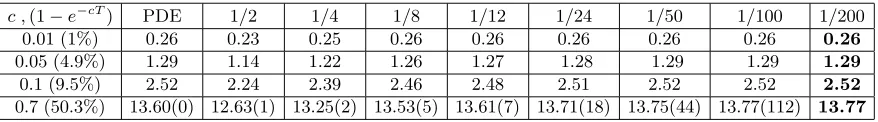
[image:23.612.75.514.629.690.2]Tables1and2). The exact value has been computed using a one-dimensional PDE solver (see
Table 1
The numerical results of E[uHJ
ω,n(0)] with the different time steps whenϕ∗(t, x) =e−c(T−t). The numbers
in the brackets indicate the CPU times (Intel Core2.60GHz) in seconds for the case c= 0.7 withN = 8192
Monte Carlo paths.
c ,(1−e−cT) PDE 1/2 1/4 1/8 1/12 1/24 1/50 1/100 1/200
0.01 (1%) 0.26 0.23 0.25 0.26 0.26 0.26 0.26 0.26 0.26
0.05 (4.9%) 1.29 1.14 1.22 1.26 1.27 1.28 1.29 1.29 1.29
0.1 (9.5%) 2.52 2.24 2.39 2.46 2.48 2.51 2.52 2.52 2.52
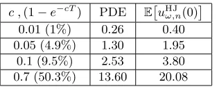
Table 2
The numerical results ofE[uHJω,n(0)]when ϕ∗(t, x) = 0.
c ,(1−e−cT) PDE E
uHJω,n(0)
0.01 (1%) 0.26 0.40 0.05 (4.9%) 1.30 1.95 0.1 (9.5%) 2.53 3.80 0.7 (50.3%) 13.60 20.08
column PDE). We have used different values ofc corresponding to a probability of default at T equal to (1−e−cT).
The approximation has two separate sources of error. First, there is the suboptimal choice of the minimizer ϕ∗ for the discretized optimization implying an upper bias. The second error arises from the discretization of the deterministic optimization problems, which could underestimate the true value of the optimization. The choice ϕ∗ =e−c(T−t) in our example— as expected—is close to being optimal, so the errors arising from the discretization dominate. To the contrary, the choice ϕ∗ = 0 is far from being optimal, so the numerical results are much bigger than the value function.
REFERENCES
[1] M. Avellaneda, A. Levy, and A. Paras, Pricing and hedging derivative securities in markets with uncertain volatilities, Appl. Math. Finance, 2 (1995), pp. 73–88.
[2] B. Bouchard and N. Touzi, Discrete-time approximation and Monte-Carlo simulation of backward stochastic differential equations, Stochastic Process. Appl., 111 (2004), pp. 175–206.
[3] P. Cheridito, M. Soner, N. Touzi, and N. Victoir, Second-order backward stochastic differential equations and fully nonlinear parabolic PDEs, Comm. Pure Appl. Math., 60 (2007), pp. 1081–1110. [4] M. H. A. Davis and G. Burstein,A deterministic approach to stochastic optimal control with application
to anticipative control, Stochastics Stochastics Rep., 40 (1992), pp. 203–256.
[5] J. Diehl, P. Friz, and P. Gassiat,Stochastic control with rough paths, preprint, arXiv:1303.7160, 2013. [6] I. Ekren, N. Touzi, and J. Zhang, Viscosity solutions of fully nonlinear parabolic path dependent
PDEs: Part II, Ann. Probab., to appear.
[7] I. Ekren, N. Touzi, and J. Zhang,Optimal stopping under nonlinear expectation, Stochastic Process. Appl., 124 (2014), pp. 3277–3311.
[8] A. Fahim, N. Touzi, and X. Warin, A probabilistic numerical method for fully nonlinear parabolic PDEs, Ann. Appl. Probab., 21 (2011), pp. 1322–1364.
[9] M. Fisher and G. Nappo,On the moments of the modulus of continuity of Itˆo processes, Stoch. Anal. Appl., 28 (2010), pp. 103–122.
[10] J. Guyon and P. Henry-Labord`ere,Uncertain volatility model: A Monte Carlo approach, J. Comput. Finance, 14 (2011), pp. 37–71.
[11] J. Guyon and P. Henry-Labord`ere,Nonlinear Option Pricing, Chapman & Hall/Financ. Math. Ser., CRC Press, Boca Raton, FL, 2014.
[12] N. V. Krylov, Approximating value functions for controlled degenerate diffusion processes by using piece-wise constant policies, Electron. J. Probab., 4 (1999), 2.
[13] N. V. Krylov, On the rate of convergence of finite-difference approximations for Bellmans equations with variable coefficients, Probab. Theory Related Fields, 117 (2000), pp. 1–16.
[14] T. Lyons,Uncertain volatility and the risk-free synthesis of derivatives, Appl. Math. Finance, 2 (1995), pp. 117–133.
[16] E. Pardoux and S. Peng, Adapted solutions of backward stochastic differential equations, Systems Control Lett., 14 (1990), pp. 55–61.
[17] L. C. G. Rogers,Pathwise stochastic optimal control, SIAM J. Control Optim., 46 (2007), pp. 1116–1132. [18] M. Soner, N. Touzi, and J. Zhang,Wellposedness of second order backward SDEs, Probab. Theory
Related Fields, 153 (2012), pp. 149–190.