This is a repository copy of Source apportionment advances using polar plots of bivariate correlation and regression statistics.
White Rose Research Online URL for this paper: http://eprints.whiterose.ac.uk/105308/
Version: Accepted Version
Article:
Grange, Stuart Kenneth, Lewis, Alastair orcid.org/0000-0002-4075-3651 and Carslaw, David Carlin orcid.org/0000-0003-0991-950X (2016) Source apportionment advances using polar plots of bivariate correlation and regression statistics. Atmospheric
Environment. pp. 128-134. ISSN 1352-2310 https://doi.org/10.1016/j.atmosenv.2016.09.016
Reuse
Items deposited in White Rose Research Online are protected by copyright, with all rights reserved unless indicated otherwise. They may be downloaded and/or printed for private study, or other acts as permitted by national copyright laws. The publisher or other rights holders may allow further reproduction and re-use of the full text version. This is indicated by the licence information on the White Rose Research Online record for the item.
Takedown
If you consider content in White Rose Research Online to be in breach of UK law, please notify us by
Source apportionment advances using polar plots of bivariate
correlation and regression statistics
Stuart K. Grangea,∗
, Alastair C. Lewisa,b
, David C. Carslawa,c
a
Wolfson Atmospheric Chemistry Laboratory, University of York, York, YO10 5DD, United Kingdom
b
National Centre for Atmospheric Science, University of York, Heslington, York, YO10 5DD, United Kingdom
c
Ricardo Energy & Environment, Harwell, Oxfordshire, OX11 0QR, United Kingdom
Abstract
This paper outlines the development of enhanced bivariate polar plots that allow the
concentrations of two pollutants to be compared using pair-wise statistics for exploring the
sources of atmospheric pollutants. The new method combines bivariate polar plots, which
provide source characteristic information, with pair-wise statistics that provide information on
how two pollutants are related to one another. The pair-wise statistics implemented include
weighted Pearson correlation and slope from two linear regression methods. The development
uses a Gaussian kernel to locally weight the statistical calculations on a wind speed-direction
surface together with variable-scaling. Example applications of the enhanced polar plots
are presented by using routine air quality data for two monitoring sites in London, United
Kingdom for a single year (2013). The London examples demonstrate that the combination
of bivariate polar plots, correlation, and regression techniques can offer considerable insight
into air pollution source characteristics, which would be missed if only scatter plots and
mean polar plots were used for analysis. Specifically, using correlation and slopes as pair-wise
statistics, long-range transport processes were isolated and black carbon (BC) contributions
to PM2.5 for a kerbside monitoring location were quantified. Wider applications and future
advancements are also discussed.
Keywords:
1. Introduction
1
Determining how variables are related to one-another is a key component of data analysis 2
and statistics. Within the atmospheric sciences, exploring the relationships between chemical 3
constituents and meteorological parameters is extremely common and the techniques for 4
comparing, correlating, and determining relationships are very diverse. Analysis involving the 5
correlation of two pollutants can often be insightful because it can lead to the identification 6
of emission source characteristics, as can investigation into ratios or slopes from regression 7
analysis between two pollutants (Statheropoulos et al.,1998). Within atmospheric disciplines, 8
data analysis can also benefit from being able to integrate wind behaviour (Elminir,2005). 9
The use of wind speed and direction can be informative because it often leads to the suggestion 10
of source locations and source characteristics, such as height of emission above the surface 11
(Henry et al., 2002; Westmoreland et al.,2007). 12
Exploration of relationships among variables can be achieved with many different methods 13
that can range from the simple to numerically complex. However, a technique that is used 14
very widely is the simple x-y scatter plot (Bentley,2004). Scatter plots are useful because 15
they allow for the visualisation of variables and model fitting can be evaluated quickly and 16
simply with visual feedback. Regression techniques, most commonly ordinary least-squared 17
regression, are often employed to formally quantify how x and y are related. The use of 18
least-squared regression is however technically questionable in many cases, and despite a 19
large collection of alternative techniques available, its use remains a persistent feature of 20
air quality data analysis. The use of simple scatter plots is usually carried out with entire 21
datasets or with simple or superficial filtering and therefore have potential to hide some 22
discrete relationships which are present in the global data if they do not conform to the 23
mean rate of change (Cade and Noon,2003). 24
Slopes from regression models relating two pollutants to one another are often used in 25
applications that use monitoring data such as emission inventories and pollutant models. 26
∗Corresponding author
When measurements are not available, slopes for the unknown pollutants are often substituted 27
from the literature, short-term monitoring, or data collected at a near-by location. However, 28
the use of simple and static ratios is likely to be deficient in many situations because they 29
can be expected to be highly dependent on source (Manoli et al., 2002). To differentiate 30
sources in air quality data, techniques other than simple scatter plots often need to be used. 31
A common method for source characterisation is the use of bivariate polar plots (Carslaw
32
et al., 2006; Westmoreland et al., 2007; Carslaw and Beevers, 2013; Uria Tellaetxe and
33
Carslaw, 2014). Polar plots are typically used to visualise and explore mean pollutant
34
concentrations for single species based on wind speed and wind direction. In the atmospheric 35
sciences, it is intuitive to plot wind direction (from 0 to 360◦ clockwise from north) on the
36
angular ‘axis’ and wind speed to be used for the radial scale. Aggregation functions other 37
than the arithmetic mean can be used and different variables apart from wind speed can be 38
used for the radial scale. For example, atmospheric temperature or stability are often useful 39
variables to use. The main attribute for the choice of radial-axis variable is that it helps to 40
differentiate between different source characteristics in some way due to different source types 41
responding differently to values of the angular scale. Despite the range of potential options, 42
wind speed is widely used to help discriminate different source types and is particularly 43
useful when used together with wind direction and the concentration of a species (Harrison
44
et al., 2001;Kassomenos et al., 2012). 45
This type of polar plot analysis has, in part, become wide-spread due to the open-source 46
polarPlot function available in the openair R package (Carslaw and Ropkins,2012;R Core
47
Team, 2016). Other similar techniques such as non-parametric wind regression have also 48
shown their ability to determine source locations for various pollutants by using polar plots 49
(Henry et al., 2002, 2009; Donnelly et al., 2011). 50
1.1. Objectives
51
Combining correlation and regression techniques with those that provide information on 52
source apportionment potentially offers considerably more insight into air pollution sources. 53
source locations and therefore different processes. It is common for emission inventories to 55
use ratios for pollutants when they are not measured or when high quality data is lacking. It 56
is hypothesised that the combination of correlation, regression, and polar plots could lead to 57
significant additions to data analysis by understanding how different pollutants are related 58
to one another depending on source. 59
In this paper, the combination of bivariate polar plots approaches with correlation and 60
regression techniques is considered for comparing two pollutants. This combination of 61
methods is then used to aid the interpretation of air quality data. The primary objectives of 62
this paper are as follows. First, to develop methods to combine bivariate polar plot techniques 63
with correlation and a range of linear regression approaches. Second, apply the methods to 64
commonly available measurements of air pollutants to demonstrate the new insights made 65
possible by these techniques. Third, to consider the wider potential uses of the approaches 66
in air quality science. The software developed has been released with an open-source licence 67
and can be found in the polarplotr R package (Carslaw and Grange, 2016). 68
2. Methods
69
2.1. Function development
70
2.1.1. Kernel weighting and scaling
71
The plotting mechanism for polar plots when using wind direction as the polar axis 72
generally involves first aggregating a time-series into wind speed and direction intervals 73
(or ‘bins’). The specific intervals and numbers of the bins can be altered for a particular 74
application, but all combinations of the two types of bins are summarised by an aggregation 75
function such as the mean or maximum. In theopenair polarPlot function, a smoothed 76
surface is fitted to these binned summaries using a generalised additive model (GAM) to 77
create a continuous surface which can be plotted with polar coordinates. Further details of 78
the approach can be found inCarslaw and Beevers (2013) and Uria Tellaetxe and Carslaw
79
(2014). 80
When applying a simple aggregation function, the number of observations in a time-series 81
visual presentation of the surface, except at the edges of the plot where there are (usually) few 83
observations. However, when calculating correlations or relationships between two variables, 84
it becomes important to consider the minimal number of observations which would create a 85
valid summary. If there are too few observations for a particular bin and a statistic such as 86
the correlation or slope is calculated between a pair of variables, it is likely that unreliable 87
summaries will be generated due to large variations between neighbouring bins. To overcome 88
this limitation, for each wind speed and direction bin, the entire time-series was evaluated 89
but observations were weighted by their proximity to a wind speed and direction bin i.e., 90
wind speed or direction values further from the bin centre are weighted less than those closer 91
to the centre of the bin. Like previous works such asHenry et al. (2002, 2009), a weighting 92
kernel was used to create weighting variables. 93
The weighting kernel used was the Gaussian kernel (Equation 1). The Gaussian kernel 94
has infinite tails and therefore all input bins are given a non-zero weighting, but observations 95
furthest from the bin being analysed have very small weights associated with them. The 96
Gaussian kernel was used for weighting both wind speed and direction because it is considered 97
more utilitarian than many other kernels such as the Epanechnikov kernel which have finite 98
bounds and therefore at times, will give observations weights of zero which can cause 99
ambiguity issues. 100
K(u) = √1
2πe
−12u2
(1)
To ensure the weighing variable was appropriate for the particular wind speed and direction 101
application, the input wind speed and direction variables required scaling. The scaling process 102
used was simple; the wind variables were multiplied by an integer to increase their bounds 103
and therefore influence within the weighting kernel. The variables were also normalised to 104
ensure that all observations had values between zero and one. This normalisation step is not 105
strictly necessary when the Gaussian kernel is used, but is needed for some other kernels and 106
ensures the output of process always had a known range. 107
was represented in the plotted surface as noise. Conversely, if weighting was extended too far, 109
isolated areas of ‘real’ peaks were obscured due to over-smoothing. It is difficult to determine 110
an optimal set of scaling values for wind speed and direction for every application, therefore 111
a series of heuristic simulations were performed to determine the ideal integer scaling values. 112
It was found that within a central range the final output was rather insensitive to the 113
scaling values. One reason for this relative insensitivity will be due to the inherent random 114
variability of concentrations as a function of either wind speed or wind direction due to 115
atmospheric turbulence. This indicates that within a central band of values, the scaling 116
process is not particularly influential. It is possible for other applications these scaling 117
magnitudes will have to be tuned and therefore the defaults can be altered by the user. 118
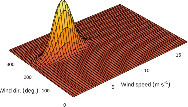
An example of the scaling defaults used in the polarPlot function are shown in Figure 1. 119
Figure1 allows visualisation of the Gaussian weighting kernel for both the wind speed and 120
direction variables as well as the extent of the default scaling procedure for a single bin for 121
4.8 m s−1 and 230 degrees.
122
5
10
15
0 100 200 300
[image:7.595.148.449.419.590.2]Windspeed(ms−1) Winddir.(deg.)
Figure 1: Three-dimensional surface of weights for a single wind speed and direction bin (4.8 m s−1and 230
degrees respectively). The surface is normalised and therefore intensity units are not informative.
After the appropriate weights have been calculated, the calculation of any pair-wise 123
statistic that allows for weighting could be calculated between two pollutants. The first 124
methods implemented were the Pearson correlation coefficient and two linear regression 125
between two pollutants and the investigation of the slope between pollutants, but with the 127
inclusion of wind speed and direction. 128
2.1.2. Correlation
129
Correlation is a measure of how well two (or more) variables are associated to one-another. 130
Correlation is a useful measure for air pollutants because pollutants which demonstrate high 131
levels of correlation are often emitted from the same source, or undergo similar chemical and 132
physical transformations in the atmosphere. For use in polar plots, the correlation statistic 133
implemented was the weighted Pearson correlation coefficient (r) (Davison and Hinkley,1997; 134
Canty and Ripley,2016). 135
2.1.3. Regression
136
Regression is a very common statistical technique and is often used to describe and 137
investigate relationships among variables (Kariya and Kurata,2004). Regression is a large 138
topic and only the linear regression techniques considered for the polar plot function will be 139
discussed. Of particular interest is the estimate of the slope from a linear regression between 140
two species. The slope will often reveal useful information concerning source characteristics, 141
for example, the amount of PM10 that is in the fine fraction (PM2.5), or the ratios of
142
combustion products such as CO and NOx which can be compared with emission inventory 143
estimates. 144
The first regression technique implemented was weighted least-squares linear regression. 145
This is very similar to ordinary least-squares linear regression, but the weighted sum of 146
squares are minimised which has the effect of creating a model which preferentially represents 147
a local area of the input data rather than the entire set. Because of the common presence of 148
outliers in air pollution time-series measurements, other regression methods such as robust 149
regression can offer advantages over the least-squares regression for use in the enhanced polar 150
plots. 151
Robust regression extends least-squares regression techniques in attempting to better 152
are violated. These violations are usually involved with the presence of outliers and het-154
eroscedasticity (non-equal variances). Primarily, the power of robust regression lies in the 155
resistance to the influence of outliers.Robust regression achieves this by substituting the 156
least-squares estimator for a more robust estimator (Yohai, 1987). There are many types of 157
robust estimators, but they all operate by first classing observations as outliers or not-outliers 158
and then reducing the influence of the outliers on the regression model (Huber,1973). The 159
procedures for calculating robust estimators are iterative and more computationally demand-160
ing when compared to the calculation of the least-squares estimator. This is noticeable to 161
a user of the polarPlot function because additional run-time is needed when the robust 162
regression techniques are used. The robust regression functions were supplied by theMASS
163
package (Venables and Ripley, 2002) and the estimator used was the M-estimator because 164
this estimator allows the use of weights. 165
2.2. Data
166
Data analysis was conducted on hourly air quality monitoring data for two sites included 167
in the United Kingdom’s Automatic Urban and Rural (AURN) Network. The two sites were 168
London Marylebone Road and London North Kensington (Table 1and Figure2). Monitoring 169
data for 2013 were downloaded using theopenair importAURNfunction. Both monitoring sites 170
measure a large complement of chemical and particulate species and achieve high data capture 171
rates. The particulate matter measurements were focused on for polar plot analysis and 172
PM10 and PM2.5 at London Marylebone Road and London North Kensington are monitored
173
by TEOM-FDMS (Tapered Element Oscillating Microbalance-Filter Dynamics Measurement 174
System) instruments. This enhanced method is not as susceptible to removing volatile and 175
semi-volatile components in the monitored air-stream as standard heated TEOMs (Allen
176
et al.,1997;Green et al.,2009). Hourly black carbon (BC) data were also used and these data 177
were sourced directly from the AURN monitoring database after personal communication 178
with Ricardo Energy & Environment. More detailed site and instrument details can be found 179
see at https://uk-air.defra.gov.uk/. 180
Table 1: Details of locations of air quality and meteorological monitoring sites in London providing data for
this study.
Site name Latitude Longitude Elevation Site type
London North Kensington 51.5211 -0.2134 5 Urban background
London Marylebone Road 51.5225 -0.1546 35 Urban traffic
London Heathrow 51.4780 -0.4610 25.3 Meteorological only
London North Kensington
London Marylebone Road
London Heathrow
0km 5km 10km
Figure 2: Locations of air quality and meteorological monitoring sites in London providing data for this
study. The map’s internal polygons show London’s Boroughs, the City of London, and the River Thames.
were used to represent regional conditions for the two air quality monitoring sites. Hourly 182
data from the London Heathrow site were obtained from the NOAA Integrated Surface 183
Database (ISD) and access was gained with the worldmet R package (NOAA, 2016; Carslaw, 184
2016). The data from Heathrow Airport were used in preference to other local surface 185
[image:10.595.132.471.249.541.2]PM2.5=PM10⋅0.87−3.7, R2=0.89
London North Kensington
0 25 50 75
0 30 60 90
HourlyPM10concentration
(
µgm− 3)
H
o
u
rl
y
P
M2.5
co
n
ce
n
tr
a
ti
o
n
(
µ
g
m
−
[image:11.595.142.456.122.431.2]3
)
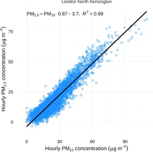
Figure 3: Simplex-y scatter plot of PM2
.5 and PM10for 2013 at London North Kensington. Fitted line and
equation represents the ordinary least-squared regression model.
3. Results & discussion
187
3.1. London North Kensington PM10 and PM2.5
188
London North Kensington is an urban background site (Table 1 and Figure 2) and it 189
is expected that a wide range of sources will contribute particle concentrations, including 190
both local (London) and long-range (continental Europe) sources. A scatter plot of PM2.5
191
and PM10 shows that the two particle size fractions showed a good degree of correlation 192
during 2013 (Figure 3). From Figure 3 alone there is no obvious indication that different 193
source types contribute to the overall scatter of points. The mean ratio between PM2.5 and
194
PM10 was 0.87, as determined by the ordinary least-squares linear regression model and it 195
The usual use of polar plots, by calculating the mean concentration for wind speed and 197
directions bins, show that the there were multiple sources of PM10 and PM2.5 at London
198
North Kensington in 2013 (Figure 4a and Figure4b). Figure 4suggests that locally-sourced 199
particulate matter were present, as potentially indicated by the elevated concentrations at 200
low wind speeds, but the highest concentrations were experienced with easterly winds when 201
wind speeds were high (≈ 10 m s−1). By contrast, NO
x, a pollutant which is dominated 202
by local (London) emissions, showed that only when wind speeds were low, were elevated 203
concentrations experienced due to a lack of pollutant dispersion (Figure 4c). However, when 204
the PM2.5 and PM10 data are plotted with a correlation statistic binned by wind speed and
205
direction, the situation is more revealing than the scatter plot and mean polar plots would 206
suggest alone (Figure5). 207 (a) 5 10 15 ws 20 W S N E
PM10 mean
PM10 10 15 20 25 30 35 40 45 50 (b) 5 10 15 ws W S N E
PM2.5 mean
PM2.5 5 10 15 20 25 30 35 40 45 (c) 5 10 15 ws 20 W S N E
NOx mean
[image:12.595.69.530.356.495.2]NOx 20 40 60 80 100 120 140 160 180
Figure 4: Polar plots of mean concentrations of PM10 (a), PM2
.5(b), and NOx(c) for 2013 at London North
Kensington.
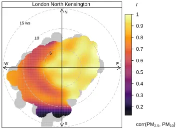
The correlation polar plot of PM2.5 and PM10 demonstrates that during easterly winds,
208
the London North Kensington PM2.5 and PM10 concentrations were very highly correlated
209
with r ≈ 0.9 (Figure5). The zone of high correlation is interpreted to be due to long-range 210
transport which is characterised by the majority of PM10being made up of PM2.5. In London,
211
and most areas of the UK, long-range transport is most important under easterly conditions 212
where air-masses originate from continental Europe (Buchanan et al.,2002;Abdalmogith and
213
Harrison, 2005; Liu and Harrison, 2011). Under these conditions the concentrations of fine 214
Figure5is also smooth and covers a wide range of wind speed and directions which indicates 216
a general, and large-scale process which is being appropriately smoothed and represented 217
by the weighting procedure (Section 2.1). Other monitoring locations, including London 218
Marylebone Road that also measure PM2.5 and PM10 showed similar easterly behaviour (not
219
shown). 220
5 10 15 ws
W
S N
E
London North Kensington r
corr(PM2.5, PM10) 0.2
[image:13.595.120.482.221.480.2]0.3 0.4 0.5 0.6 0.7 0.8 0.9 1
Figure 5: Polar plot of the correlation between PM2
.5and PM10 for 2013 at London North Kensington.
Previous studies such as Querol et al.(2004); Charron and Harrison(2005);Harrison et al.
221
(2001); Liu and Harrison(2011) have reported high PM2.5–PM10 ratios for European sourced
222
particulate matter in the UK and the correlation presented in Figure5is consistent with these 223
past works which reported high PM2.5–PM10 ratios. When HYSPLIT (Stein et al., 2015)
224
back-trajectories for 2013 were clustered and joined to coincident pollutant observations, the 225
cluster representing air-masses from Europe also had the highest PM2.5–PM10 ratio of all
226
clusters, consistent with the conclusions inferred from Figure 5. 227
The polar plot of the slope between PM2.5 and PM10 at London North Kensington
228
demonstrates a similar surface pattern as the correlation polar plot (Figure 6). The long-229
range sourced particulate from the east was indeed primarily composed of PM2.5, as shown
by a PM2.5 to PM10 slope of about 90 %. For other wind directions, coarser particulate
231
matter was a more important contributor to PM10 and the PM2.5 contributions drop to
232
approximately 30 % (Figure6). This reduction of PM2.5 to PM10slope was most likely caused
233
the local process of mechanical resuspension. Even though the scatter plot of PM2.5 and
234
PM10 (Figure 3) does not indicate different source influences, it is clear from Figure 6 in 235
particular that there are at least two major source types affecting particulate concentrations 236
at the London North Kensington site. It should be noted that a careful wind speed, wind 237
direction subset of the data shown in Figure 3does confirm the behaviour seen in Figure 6
238
with a much lower PM2.5 to PM10 slope for south-westerly winds above 5 m s−
1. 239
5 10 15 ws
W
S N
E Formula:
PM2.5 ~ PM10
London North Kensington
robust
slope
[image:14.595.144.450.311.582.2]PM2.5 PM10 0.3 0.4 0.5 0.6 0.7 0.8 0.9 1
Figure 6: Polar plot of the robust slope between PM2
.5 and PM10 for 2013 at London North Kensington.
3.2. London Marylebone PM2.5 and BC
240
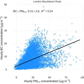
Unlike PM10 and PM2.5 at London North Kensington, the London Marylebone Road BC
241
and PM2.5 correlation was poor in 2013, as shown in Figure 7. Although BC exists primarily
242
BC=PM2.5⋅0.21+2.6, R 2
=0.24
London Marylebone Road
0 10 20 30 40 50
0 25 50 75 100
HourlyPM2.5concentration
(
µgm− 3)
H
o
u
rl
y
B
C
co
n
ce
n
tr
a
ti
o
n
(
µ
g
m
−
[image:15.595.152.449.119.416.2]3
)
Figure 7: Simplex-y scatter plot of BC and PM2
.5 for 2013 at London Marylebone Road. Fitted line and
equation represents the ordinary least-squared regression model.
expected to be an important component of PM2.5 at a traffic-dominated location like London
244
Marylebone Road, PM2.5 also has a diverse number of other sources including secondary
245
inorganic aerosol (Querol et al., 2004). Therefore, at times, BC will be a major contributor 246
to PM2.5 while at others it will be a minor component depending on the strength of the
247
various sources. Using a scatter plot to investigate this relationship is not immediately useful 248
because the two variables do not follow a mean rate of change. Therefore, fitting a simple 249
linear regression line to these data is not informative (Figure 7). 250
The robust regression slope of BC and PM2.5 binned by wind speed and direction at
251
London Marylebone Road demonstrated patterns that were not observed by the simple 252
scatter plot alone (Figure8a). Figure 8a shows that the ratio between BC and PM2.5 was
253
Road had a higher ratio of BC with ≈ 50 % of PM2.5 being composed of BC. BC-PM2.5
255
ratios are sparsely reported, however London Marylebone Road’s ratio is consistent with 256
what Ruellan and Cachier (2001) reported for a traffic-dominated monitoring location in
257
Paris (Porte d’Auteuil) with ratios of 43 ± 20 %. When winds were from the north and 258
westerly directions, the BC-PM2.5 ratio was lower, usually under 20 %. Additionally, winds
259
from the north were nearly completely free of BC particulate matter (Figure8a). 260
(a)
5 10 15 ws 20
W
S N
E Formula:
BC ~ PM2.5
robust slope
BC PM2.5
0.1 0.2 0.3 0.4 0.5 0.6
(b)
5 10 15 ws
W
S N
E Formula:
BC ~ PM2.5
robust slope
BC PM2.5
0.02 0.04 0.06 0.08 0.1 0.12 0.14
[image:16.595.65.532.248.462.2]London Marylebone Road London North Kensington
Figure 8: Polar plot of the robust slope between BC and PM2
.5 at London Marylebone Road (a) and London
North Kensington (b).
The wind direction dependencies inferred from the polar plot are somewhat counter-261
intuitive given that the London Marylebone Road monitoring site is located one metre from 262
the kerb on the south-side of an arterial road. However, the site is also within a significant 263
street-canyon with a width of 40 m and a height of 41 m which is likely to lead to complex 264
recirculation patterns at a range of wind speeds (Charron and Harrison,2005; Giorio et al., 265
2015). Based on this evidence, accumulation of pollutants on the buildings’ lee-side (south) 266
is an important process to consider at London Marylebone Road when interpreting source 267
processes. 268
London North Kensington also measures BC and PM2.5 and the slope of these two
(Figure8b). London North Kensington is an urban background site and lacks the large traffic 271
source being in immediate proximity which London Marylebone Road experiences. Therefore, 272
BC was a much smaller component of PM2.5. In 2013, London North Kensington had a
273
maximum contribution of ≈ 15 % of BC to PM2.5 (Figure 8b). However, this maximum
274
contribution only occurred when wind speeds were low and suggests that this contribution is 275
reached only when local traffic emissions influence the monitoring site. 276
Based on these results for the two monitoring sites, the clear and consistent BC-PM2.5
277
ratio at London Marylebone Road of around 50 % shown in Figure 8a in the south-west 278
quadrant can be interpreted as a contribution dominated by local traffic sources. The lower 279
ratio of between 10–20 % mostly to the east is dominated by regional source contributions 280
where the concentration of PM2.5 is relatively high but where air masses contain very little
281
BC. 282
3.3. Future directions
283
The examples presented for a single year of data for two air quality monitoring sites 284
in London were the first steps for enhancing polar plots to include the functionality of 285
pair-wise statistics. The enhancements were able to substantially improve the information 286
content available from routinely monitored air pollutants where simple scatter plots and 287
‘standard’ polar plots gave no suggestion of the processes subsequently illuminated by the 288
correlation/slope polar plots. 289
The examples reported were for a few commonly measured species. However, it is expected 290
that the use of polar plots using pair-wise statistics for multi-species data such as metal 291
or VOC concentrations could be highly informative. Measurement of large numbers of 292
metals and other species at higher time resolutions (hourly) is becoming more common. 293
A ‘correlation matrix of robust slope polar plots’ would potentially reveal more detailed 294
information on common source origins. 295
The use of other statistics is another valuable future direction such as non-parametric 296
measures of correlation such as Spearman. Other regression techniques such as quantile 297
across a range of quantile levels, potentially providing more comprehensive information on 299
the relationship between two pollutants and give further options when determining pollutant 300
sources. The main advantage of quantile regression is likely to be related to resolving two 301
or more sources that overlap and where there is not a single dominant slope caused by 302
one source. In this case, considering the full distribution of slope values may help better 303
resolve competing source contributions. Finally, the weighted statistics approach for paired 304
statistics could usefully be extended to model evaluation where two sets of data are compared 305
(observed and modelled). In this case, enhanced polar plot analyses could provide valuable 306
information concerning where model agreement is good or poor and indicate more clearly the 307
conditions under which model performance is acceptable and provide enhanced information 308
on where model performance is poor. 309
4. Conclusions
310
This paper outlined the development of enhanced bivariate polar plots to include pair-wise 311
statistics to be used in the atmospheric sciences. Two groups of statistical techniques were 312
implemented: correlation and regression. The new development brings together commonly 313
used pair-wise statistics and relationships with wind speed and direction, which provides 314
enhanced information on pollutant sources beyond currently used techniques. 315
Using a single year of data, in a single city, for routinely monitored pollutants demonstrated 316
that the enhanced polar plots were capable of determining relationships and processes that 317
were not suggested by simple scatter plots and the use of mean polar plots alone. Here we 318
have reported that traffic dominated PM2.5 is composed of 50 % BC at a London monitoring
319
site. This is an important observation and ratios between other pollutants such as elemental 320
carbon and organic carbon (EC and OC) is an obvious future application for the enhanced 321
polar plots. 322
It is expected in the future that enhanced polar plots will be widely used for the 323
investigation of ratios for pairs of pollutants and further extended to be a valuable tool for 324
Acknowledgements
326
This work was supported by Anthony Wild with the provision of the Wild Fund Scholarship. 327
This work was also partially funded by the 2016 Natural Environment Research Council 328
(NERC) air quality studentships programme. 329
Highlights
330
• Bivariate polar plots are a common method for exploring pollutant sources. 331
• Polar plots were enhanced with the addition of pair-wise statistics. 332
• Usage examples of the enhanced polar plots are given for two London monitoring sites. 333
• Processes were illuminated that were not detected by other plotting methods. 334
• Potential future applications and extensions are discussed for bivariate polar plots. 335
References
336
Abdalmogith, S. S., Harrison, R. M., 2005. The use of trajectory cluster analysis to examine the long-range 337
transport of secondary inorganic aerosol in the UK. Atmospheric Environment 39 (35), 6686–6695. 338
URLhttp://www.sciencedirect.com/science/article/pii/S1352231005006825
339
Allen, G., Sioutas, C., Koutrakis, P., Reiss, R., Lurmann, F. W., Roberts, P. T., 1997. Evaluation of the 340
TEOM method for measurement of ambient particulate mass in urban areas. Journal of the Air & Waste 341
Management Association 47 (6), 682–689. 342
Bentley, S., 2004. Graphical techniques for constraining estimates of aerosol emissions from motor vehicles 343
using air monitoring network data. Atmospheric Environment 38 (10), 1491–1500. 344
URLhttp://www.sciencedirect.com/science/article/pii/S1352231003010574
345
Buchanan, C., Beverland, I., Heal, M., 2002. The influence of weather-type and long-range transport on 346
airborne particle concentrations in Edinburgh, UK. Atmospheric Environment 36 (34), 5343–5354. 347
URLhttp://www.sciencedirect.com/science/article/pii/S1352231002005794
348
Cade, B. S., Noon, B. R., 2003. A gentle introduction to quantile regression for ecologists. Frontiers in 349
Ecology and the Environment 1 (8), 412–420. 350
URLhttp://dx.doi.org/10.1890/1540-9295(2003)001[0412:AGITQR]2.0.CO;2
351
Carslaw, D., 2016. worldmet: Import Surface Meteorological Data from NOAA Integrated Surface Database 353
(ISD). R package version 0.6. 354
URLhttp://github.com/davidcarslaw/worldmet
355
Carslaw, D., Grange, S., 2016. polarplotr: Functions to plot polar-plots. R package. 356
URLhttps://github.com/davidcarslaw/polarplotr
357
Carslaw, D. C., Beevers, S. D., 2013. Characterising and understanding emission sources using bivariate 358
polar plots and k-means clustering. Environmental Modelling & Software 40, 325–329. 359
URLhttp://www.sciencedirect.com/science/article/pii/S136481521200237X
360
Carslaw, D. C., Beevers, S. D., Ropkins, K., Bell, M. C., 2006. Detecting and quantifying aircraft and 361
other on-airport contributions to ambient nitrogen oxides in the vicinity of a large international airport. 362
Atmospheric Environment 40 (28), 5424–5434. 363
URLhttp://www.sciencedirect.com/science/article/pii/S1352231006004250
364
Carslaw, D. C., Ropkins, K., 2012.openair — An R package for air quality data analysis. Environmental 365
Modelling & Software 27–28 (0), 52–61. 366
URLhttp://www.sciencedirect.com/science/article/pii/S1364815211002064
367
Charron, A., Harrison, R. M., 2005. Fine (PM2
.5) and Coarse (PM2.5−10) Particulate Matter on A Heavily
368
Trafficked London Highway: Sources and Processes. Environmental Science & Technology 39 (20), 7768– 369
7776. 370
URLhttp://dx.doi.org/10.1021/es050462i
371
Davison, A. C., Hinkley, D. V., 1997. Bootstrap Methods and Their Applications. Cambridge University 372
Press, Cambridge, ISBN 0-521-57391-2. 373
URLhttp://statwww.epfl.ch/davison/BMA/
374
Donnelly, A., Misstear, B., Broderick, B., 2011. Application of nonparametric regression methods to study 375
the relationship between NO2 concentrations and local wind direction and speed at background sites. 376
Science of The Total Environment 409 (6), 1134–1144. 377
URLhttp://www.sciencedirect.com/science/article/pii/S0048969710012726
378
Elminir, H. K., 2005. Dependence of urban air pollutants on meteorology. Science of The Total Environment 379
350 (1–3), 225–237. 380
URLhttp://www.sciencedirect.com/science/article/pii/S0048969705000732
381
Giorio, C., Tapparo, A., Dall’osto, M., Beddows, D. C. S., Esser Gietl, J. K., Healy, R. M., Harrison, R. M., 382
2015. Local and Regional Components of Aerosol in a Heavily Trafficked Street Canyon in Central London 383
Derived from PMF and Cluster Analysis of Single-Particle ATOFMS Spectra. Environmental Science & 384
Technology 49 (6), 3330–3340. 385
URLhttp://dx.doi.org/10.1021/es506249z
Green, D. C., Fuller, G. W., Baker, T., 2009. Development and validation of the volatile correction model 387
for PM10—An empirical method for adjusting TEOM measurements for their loss of volatile particulate 388
matter. Atmospheric Environment 43 (13), 2132–2141. 389
URLhttp://www.sciencedirect.com/science/article/pii/S1352231009000557
390
Harrison, R. M., Yin, J., Mark, D., Stedman, J., Appleby, R. S., Booker, J., Moorcroft, S., 2001. Studies of 391
the coarse particle (2.5–10µm) component in UK urban atmospheres. Atmospheric Environment 35 (21), 392
3667–3679. 393
URLhttp://www.sciencedirect.com/science/article/pii/S1352231000005264
394
Henry, R., Norris, G. A., Vedantham, R., Turner, J. R., 2009. Source Region Identification Using Kernel 395
Smoothing. Environmental Science & Technology 43 (11), 4090–4097. 396
URLhttp://dx.doi.org/10.1021/es8011723
397
Henry, R. C., Chang, Y.-S., Spiegelman, C. H., 2002. Locating nearby sources of air pollution by nonparametric 398
regression of atmospheric concentrations on wind direction. Atmospheric Environment 36 (13), 2237–2244. 399
URLhttp://www.sciencedirect.com/science/article/pii/S1352231002001644
400
Huber, P. J., 1973. Robust regression: asymptotics, conjectures and Monte Carlo. The Annals of Statistics, 401
799–821. 402
Kariya, T., Kurata, H., 2004. Generalized least squares. John Wiley & Sons. 403
Kassomenos, P., Vardoulakis, S., Chaloulakou, A., Grivas, G., Borge, R., Lumbreras, J., 2012. Levels, sources 404
and seasonality of coarse particles (PM10–PM2
.5) in three European capitals — Implications for particulate
405
pollution control. Atmospheric Environment 54 (0), 337–347. 406
URLhttp://www.sciencedirect.com/science/article/pii/S1352231012001665
407
Koenker, R., Bassett, Jr, G., 1978. Regression quantiles. Econometrica: journal of the Econometric Society, 408
33–50. 409
Liu, Y.-J., Harrison, R. M., 2011. Properties of coarse particles in the atmosphere of the United Kingdom. 410
Atmospheric Environment 45 (19), 3267–3276. 411
URL http://www.sciencedirect.com/science/article/B6VH3-52G8GT9-1/2/
412
1c4d705b78225fca7c930197cd80c35a
413
Manoli, E., Voutsa, D., Samara, C., 2002. Chemical characterization and source identification/apportionment 414
of fine and coarse air particles in Thessaloniki, Greece. Atmospheric Environment 36 (6), 949–961. 415
URLhttp://www.sciencedirect.com/science/article/pii/S1352231001004861
416
NOAA, 2016. Integrated Surface Database (ISD). 417
URLhttps://www.ncdc.noaa.gov/isd
418
Petzold, A., Kopp, C., Niessner, R., 1997. The dependence of the specific attenuation cross-section on black 419
URLhttp://www.sciencedirect.com/science/article/pii/S1352231096002452
421
Querol, X., Alastuey, A., Ruiz, C., Artiano, B., Hansson, H., Harrison, R., Buringh, E., ten Brink, H., Lutz, 422
M., Bruckmann, P., Straehl, P., Schneider, J., 2004. Speciation and origin of PM10 and PM2.5 in selected 423
European cities. Atmospheric Environment 38 (38), 6547–6555. 424
URLhttp://www.sciencedirect.com/science/article/pii/S1352231004008143
425
R Core Team, 2016. R: A Language and Environment for Statistical Computing. R Foundation for Statistical 426
Computing, Vienna, Austria. 427
URLhttps://www.R-project.org/
428
Ruellan, S., Cachier, H., 2001. Characterisation of fresh particulate vehicular exhausts near a Paris high flow 429
road. Atmospheric Environment 35 (2), 453–468. 430
URLhttp://www.sciencedirect.com/science/article/pii/S1352231000001102
431
Statheropoulos, M., Vassiliadis, N., Pappa, A., 1998. Principal component and canonical correlation analysis 432
for examining air pollution and meteorological data. Atmospheric Environment 32 (6), 1087–1095. 433
URLhttp://www.sciencedirect.com/science/article/pii/S1352231097003774
434
Stein, A. F., Draxler, R. R., Rolph, G. D., Stunder, B. J. B., Cohen, M. D., Ngan, F., 2015. NOAA’s HYSPLIT 435
Atmospheric Transport and Dispersion Modeling System. Bulletin of the American Meteorological Society 436
96 (12), 2059–2077. 437
URLhttp://dx.doi.org/10.1175/BAMS-D-14-00110.1
438
Uria Tellaetxe, I., Carslaw, D. C., 2014. Conditional bivariate probability function for source identification. 439
Environmental Modelling & Software 59 (0), 1–9. 440
URLhttp://www.sciencedirect.com/science/article/pii/S1364815214001339
441
Venables, W. N., Ripley, B. D., 2002. Modern Applied Statistics with S, 4th Edition. Springer, New York, 442
ISBN 0-387-95457-0. 443
URLhttp://www.stats.ox.ac.uk/pub/MASS4
444
Viidanoja, J., Sillanp¨a¨a, M., Laakia, J., Kerminen, V.-M., Hillamo, R., Aarnio, P., Koskentalo, T., 2002. 445
Organic and black carbon in PM2
.5 and PM10: 1 year of data from an urban site in Helsinki, Finland.
446
Atmospheric Environment 36 (19), 3183–3193. 447
URLhttp://www.sciencedirect.com/science/article/pii/S1352231002002054
448
Westmoreland, E. J., Carslaw, N., Carslaw, D. C., Gillah, A., Bates, E., 2007. Analysis of air quality within 449
a street canyon using statistical and dispersion modelling techniques. Atmospheric Environment 41 (39), 450
9195–9205. 451
URLhttp://www.sciencedirect.com/science/article/pii/S1352231007006863
452
Yohai, V. J., 1987. High Breakdown-Point and High Efficiency Robust Estimates for Regression. The Annals 453
URLhttp://www.jstor.org/stable/2241331