This is a repository copy of
An Alternative for PID control: Predictive Functional Control - A
Tutorial
.
White Rose Research Online URL for this paper:
http://eprints.whiterose.ac.uk/109310/
Version: Accepted Version
Proceedings Paper:
Haber, R., Rossiter, J.A. orcid.org/0000-0002-1336-0633 and Zabet, K.R. (2016) An
Alternative for PID control: Predictive Functional Control - A Tutorial. In: American Control
Conference (ACC), 2016. ACC2016, 06-08 Jul 2016, Boston, MA, USA. IEEE .
https://doi.org/10.1109/ACC.2016.7526765
[email protected] https://eprints.whiterose.ac.uk/ Reuse
Unless indicated otherwise, fulltext items are protected by copyright with all rights reserved. The copyright exception in section 29 of the Copyright, Designs and Patents Act 1988 allows the making of a single copy solely for the purpose of non-commercial research or private study within the limits of fair dealing. The publisher or other rights-holder may allow further reproduction and re-use of this version - refer to the White Rose Research Online record for this item. Where records identify the publisher as the copyright holder, users can verify any specific terms of use on the publisher’s website.
Takedown
If you consider content in White Rose Research Online to be in breach of UK law, please notify us by
Abstract— PFC (Predictive Function Control) can be
considered as a bridge between PI(D) and complex MPC. PI(D) control can have problems handling dead time and constraints. PFC handles these cases and is often better than using a Smith predictor. PFC is a simple realizable MPC which thus uses prediction and preview of key variables. PFC can be implemented via simple program code and thus has cheap license costs. The tutorial introduces the basic idea of PFC and algorithms for typical processes. Simulations illustrate its effectiveness and advantages over PI(D) and Smith predictors.
I. INTRODUCTION
PI(D) (Proportional-Integral-Derivative) control is well known in the industry, as most controllers are of this type. On the other side the PID parameters cannot be tuned easily for fastest aperiodic settling and its usage is limited by dead times. One extension for dead time processes is to deploy alongside a Smith predictor. However this mechanism is sensitive to parameter changes.
Richalet [1] introduced PFC (Predictive Functional Control) as an alternative to PID for processes having dead time and was able to implement on available processors in the 1960s! The manipulating variable (MV) is defined as the sum of weighted basis functions and is calculated by minimizing a sum of quadratic terms of control errors at so called coincidence points in the future. Instead of weighting the control increments, the difference between a reference trajectory and the controlled signal is weighted exponentially. If the reference signal and the disturbance change only stepwise, then just one basis function and one coincidence point are required and the MV is calculated from an algebraic equation.
The advantage of PFC over PI(D) control is the embedded ability to control dead time processes and to constrain both the manipulated and the controlled signal. In addition the tuning parameters have physical meaning which helps in introducing the algorithm in practice. One of the parameters tunes the robustness, as well.
For big plants, like refineries, the process industry uses MPC (Model Predictive Control) which uses a complex numerical optimization of the actual and future manipulated variable sequence by taking into account different constraints. The main drawback of MPC is that the
1 R. Haber and K. Zabet, Laboratory of Process Control, Institute of Process Engineering and Plant Design, Faculty of Process Engineering, Energy and Mechanical Systems, Cologne University of Applied Science, D-50679 Köln, Germany, (e-mail: [email protected]).
2 J. A. Rossiter is with Dept. of Automatic Control and Systems Eng., University of Sheffield, S1 3JD, UK (e-mail: [email protected]).
algorithm considering constraints is so complex that the implementation requires expert knowledge and commercial programs have to be installed with a correspondingly high cost license fee.
Where the task is to improve the behavior of low-level, basic controllers only, PFC in its simplified version is a good choice because of both calculation and tuning simplicity and also its easy implementation and capability of constraints handling. The presented PFC algorithm of course cannot replace a multivariable, robust, stable, constrained MPC. Both algorithms have their different field of application.
As PFC uses an easy algorithm, any engineer can write the program code and no license has to be paid. Because of all these advantages PFC has been applied in the process industry very frequently, mainly as an easily tunable and more robust controller for nonlinear and dead-time processes than PI(D). PFC applications are present in many different countries with many different types of processes. PFC is taught in several technical schools and it is implemented in different forms for different scenarios.
II. BASIC IDEA OF PFC
The basic idea is shown first for a SISO (Single-Input, Single-Output) first-order process having no dead time and when a stepwise change of the set-point should be followed. The principle of PFC is that the controlled variable y
achieves the reference trajectory at the target point (or points) using one change (or minimal number of changes) in the MV (here denoted by u). The desired change in the controlled variable y during the prediction horizon np (from the actual time k) is calculated from the desired change of the reference trajectory and the predicted change of a model output ym. The MV can be calculated easily from the change of the reference trajectory and the predicted change of the model output during the prediction horizon, see Fig.1. The desired changes in the controlled variable y during np prediction step can be defined supposing that y matches the reference trajectory at the target point (np steps ahead):
) | ( ˆ ) ( ) ( ) | (
ˆ k n k y k ek e k n k
y p p (1)
where e(k)yr y(k) and yr is the assumed constant reference signal.
The reference trajectory is chosen to be an exponential function for simplicity. Then the tracking error is decreasing monotonically:
) ( ) | ( ˆ , ), ( ) | 1 (
ˆ k k e k e k n k ek
e np
r p
r
(2)
An Alternative for PID control: Predictive Functional Control -
A Tutorial
Fig. 1. PFC principle
where r is the reduction ratio of the trajectory’s error. The
reference trajectory is linked to the desired settling time
t95%=Tc for the closed loop control system ifr exp
3t Tc
, where t is the sampling time. From (1) and (2), the desired change in y is defined as follows:)] ( )[ 1 ( ) ( ) 1 ( ) | (
ˆ k n k e k y y k
y r n r n r p p
p
(3)which should be equal to the change in the model output.
)
(
)
|
(
ˆ
)
|
(
ˆ
k
n
k
y
k
n
k
y
k
y
m
p
m
p
m
(4)Remark 1: With a stepwise change in the reference (or disturbance) signal, a constant MV can be assumed. With another type of reference signal (e.g. sum of polynomial functions) the MV consists of similar, so called basic, functions; the name PFC arises from this expression. In this case a (quadratic) cost function has to be minimized which includes the sum of squares of the predicted control errors in different, so called coincidence, points [2].
III. PFCALGORITHM FOR SISOPROCESSES
A. First-order Process without Dead Time
The difference equation of a 1st order model is
) 1 ( ) 1 ( ) 1 ( )
(k a y k K a u k
ym m m m m (5)
where ym is the model output, u is the model input, am is the discrete-time model parameter and Km is the static gain of the model. Supposing that the actual input signal u is kept constant during the prediction horizon, then the predicted model output after np steps is:
) ( ] ) ( 1 [ ) ( ) ( ) |
(k n k a y k K a u k
y p np
m m m n m p
m (6)
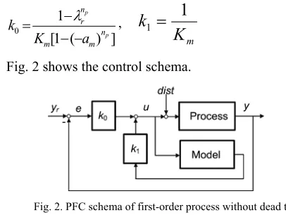
Ensuring equality between the predicted change of the reference trajectory in (3) and the predicted change of ym in (4) results in the manipulated variable (or control law):
) ( )] ( [ )
(k k0 y y k k1y k
u r m
(7a) ] ) ( 1 [ 1 0 p p n m m n r a K k , m
K
k
1
1
(7b)Fig. 2 shows the control schema.
Fig. 2. PFC schema of first-order process without dead time
B. First-order Process with Dead Time
In case of dead time dm, y(k) has to be replaced by
) | (
ˆ k d k
y m in equation (7a). The difference between the delayed and current process output is approximated by the difference between the current and earlier delayed model output values. ) ( ) ( ) ( ) | (
ˆ k dm k yk ym k ym k dm
y (8)
This approximation leads to
( ) ( )
) ( ) | (ˆ k dm k yk ym k ym k dm
y
(9)
B. Second-order Aperiodic Process
[image:3.612.93.259.59.236.2]A second-order aperiodic process can be described by a parallel connection of two first-order processes with different time constants, as shown in Fig. 3.
Fig. 3. Parallel connection of two first-order models
The difference equation of the i-th sub-model is
) 1 ( ) 1 ( ) 1 ( ) ( , , , ,
, k a y k K a u k
ymi mi mi mi mi (10)
The gains of the sub-models can be calculated by partial fraction decomposition ) 1 ( ) 1 ( ) 1 )( 1 ( 2 2 1 1 2 1 m m m m m m m sT K sT K sT sT K
(11)
(If the process has multiple poles then different but very similar poles are used.) Substituting the predictions from (10) into (7a), the PFC control law becomes
) ( ) ( )] ( [ )
(k k0 y y k k1y 1 k k2y 2 k
u r m m (12)
] ) ( 1 [ ] ) ( 1 [ 1 2 2 1 1
0 p p
p n m m n m m n a K a K k , ] ) ( 1 [ ] ) ( 1 [ ) ( 1 2 2 1 1 1 1 p p p n m m n m m n m a K a K a k
[image:3.612.384.491.421.489.2]] ) ( 1 [ ] ) ( 1 [
) ( 1
2 2
1 1
2 2
p p
p
n m m
n m m
n m
a K
a K
a k
Fig. 4 shows the control of a second-order process with the process/model parameters Km = 1, Tm1 = 1/3s, Tm2 = 2/3s without dead time, t=0.05s, np=10 and different desired settling times. It is clear that the control is aperiodic, faster control results in large initial MV and the settling time approximates the controller parameter Tc, as expected.
Remark 2: In the case of an underdamped process the transfer function can be decomposed in a similar way as with aperiodic processes, but the time constants and gains of the sub-models are pairwise complex conjugate. It can be shown that the control algorithm (13) is still valid and some parameters are complex. The MV is (of course) real.
0 2 4 6 8 10 12
-0.5 0 0.5 1 1.5
t
yr
,y
0 2 4 6 8 10 12
0 1 2 3
t
u
yref z y(T
c=0.5)
y(Tc=2) y(Tc=5)
[image:4.612.352.530.58.200.2]u(Tc=0.5) u(Tc=2) u(Tc=5)
Fig. 4. PFC of a second-order aperiodic process
C. Higher-order Processes Including Dead time
Chemical, heating, ventilating and air conditioning plants are often described by an aperiodic process of higher order. The same technique as with second-order processes can be applied [3]. Also dead-time can be considered as in (9).
IV. TUNING OF CONTROLLER PARAMETERS
The course of the controlled variable depends on:
np: prediction horizon
r: reduction ratio of the successive control errors Richalet [2] recommends the choice of the prediction horizon as for first-order processes np=1,
the discrete-time point of the inflection point of the step response for aperiodic processes of higher order. Fig. 5 shows the choice of np=10 steps (inflection point at 10· t=0.05s=0.5s) from the steps and pulse responses of the simulated second-order process.
Remark 3: These tuning recommendation work well for first-order processes, and also for aperiodic ones, but can cause big overshoots or even instability when applied for some processes, such as with underdamping. In [4] several examples are shown of this problem. Fortunately a lot of industrial processes are aperiodic, like heating, cooling, etc.
0 1 2 3 4 5 6
0 0.5 1
Process step response
0 1 2 3 4 5 6 7
0 0.01 0.02 0.03 0.04
Process pulse response (np = 10)
Fig. 5. Choice of the prediction length for the 2nd-order process
V. CONSTRAINT HANDLING
A. Constraints on the Manipulated Variable
Both the MV and its increment can be limited easily. It is important that the process model is fed by the limited MV. This kind of MV limitation is much easier than an anti-windup technique with PI control. Fig. 6 shows the level and the speed limiter [5].
Fig. 6a. The manipulated variable level limiter
Fig. 6b. The manipulated variable speed limiter
B. Constraints on the Controlled Variable
[image:4.612.71.295.244.434.2]Fig. 7. Handling constraints on the controlled signal
VI. PROGRAM CODE OF THE PFCALGORITHM
The list gives exemplars of real-time computation Matlab code based on a second-order process with dead time taking MV constraints into account.
ym1(k)=-am1*ym1(k-1)+Km1*bm1*u(k-1);
%PT1 sub-model-1 output; bm1=1+am1
ym2(k)=-am2*ym2(k-1)+Km2*bm2*u(k-1); %PT1 sub-model-2 output; bm2=1+am2
ym(k)=ym1(k)+ym2(k);% PT2 model output
u(k)=(yref(k)-(y(k)+(ym(k)-ym(k-dm)))) *k0+ym1(k)*k1+ym2(k)*k2; % MV
if u(k)> umax, u(k)=umax; end; %MV-max
if u(k)< umin, u(k)=umin; end; %MV-min
if u(k)>u(k-1)+ dumax,
u(k)=u(k-1)+ dumax; %MV-incr-max
else if u(k)<u(k-1)+ dumin,
u(k)=u(k-1)+ dumin; %MV-incr-min
end; end;
It is seen that the code for implementing a PFC control law is simple and no anti-windup calculation is necessary.
VII. COMPARISON WITH PI(D)CONTROL
[image:5.612.321.552.102.235.2]In a boiler the cold water increase leads temporarily to a decrease of the level as bubbles in the boiling water collapse. If the water feed becomes warmer, the level increases and achieves its new, higher steady-state value. Such a process is called inverse repeat or non-minimum-phase one, see Fig. 8. Fig. 9 shows PID and PFC control, respectively. In both cases standard tuning rules were used. It is clear that PFC performs better. Table 1 compares PFC to PI(D).
Fig. 8. Level step response of a boiler
VIII. COMPARISON WITH SMITH PREDICTOR
Dead time processes can be controlled using a Smith predictor, see Fig. 10.
If process model is equivalent to process and there is no disturbance then the controller sees only the model without
dead time. The controller can be designed for the dead-time- free process and the controlled output is delayed by the dead time. The problem of a Smith predictor is that it is very sensitive to process and model mismatch (see Table 2).
Fig. 9. PFC vs. PID level control of the boiler
Table 1. PFC vs. PI(D)
Feature PI(D) PFC
Dead time Cannot handle Can handle
MV constraint Anti-windup algorithm Simple clipping
Controller tuning
Common tuning rules not appropriate
Desired settling time is control parameter
CV constraint Not possible Using CV prediction
Robustness Basic algorithm not Yes, via settling time
Set-point pred. Not Possible
Fig. 10. Smith predictor
With a stepwise reference signal change it can be shown that PFC for processes with dead time has the form of a Smith predictor. This is illustrated here for a first-order system, see (7) and (9):
) ( )] | ( ˆ [ )
(k k0 y y k d k k1y k
u r m m (14)
IX. ROBUST PFC
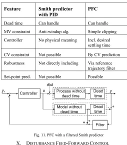
[image:5.612.307.561.290.493.2] [image:5.612.73.280.556.639.2]Table 2. PFC vs. Smith predictor with PI(D)
Feature Smith predictor with PID
PFC
Dead time Can handle Can handle
MV constraint Anti-windup alg. Simple clipping
Controller No physical meaning Incl. desired settling time
CV constraint Not possible By CV prediction
Robustness Not directly including Via reference trajectory filter
[image:6.612.46.300.64.354.2]Set-point pred. Not possible Possible
Fig. 11. PFC with a filtered Smith predictor
X. DISTURBANCE FEED-FORWARD CONTROL
A.Measured Disturbance Feed-forward Control
Assume an additive output disturbance. Its compensation is possible if the dead time of the disturbance process is greater than (or equal to) the dead time of the process. For simplicity consider the case of first-order model (1) with dead time d and disturbance model with dead time dv≥d.
) 1 ( ) 1 ( ) 1 ( )
(k a y k K a v k
yvm vm vm vm vm m (15)
The MV can be calculated [5] with k0, k1 from (7b) and
)) ( ( )) ( ( ) ( )]}] ( )) ( ( [ )] ( ) ( [ ) ( { [ ) ( 2 1 1 0 d d k y k d d k v k k y k d k y d d k y d k y k y k y y k k u v vm v v m v m v vm v vm m m r (16) ] ) ( 1 [ ] ) ( 1 [ 1 p p n m m n vm vm v a K a K k
;
] ) ( 1 [ ) ( 1 2 p p n m m n vm v a K a k (17)
Fig. 12 shows the simulation of PFC with feed-forward based on the measured disturbance. A delayed first-order model of these processes is assumed in the PFC algorithm with Km = 2, Tm = 10s, and Tdm = 10s. The controller parameters are Tc=25s and np=1. The control scenario in Figs. 12 and later in Fig. 14 is:
sampling time t=1s and simulation time = 460s,
at t=10s stepwise increase of yr from 0 to 1,
at t=160s stepwise external disturbance (0 -0.5).
at t=310s stepwise increase of process gain by 50%.
B.Estimated Disturbance Feed-forward Control
Richalet [2] introduced the disturbance observer (Fig. 13). The main advantage of this scheme is that it uses
[image:6.612.324.542.299.638.2]same tools as the already installed PFC, which thus can be implemented easily. A simulated process model is controlled by a fast PFC in the estimator. Both the “real” controller and the estimator controller use the same process model without dead time. The controlled variable y is applied as the reference signal of the estimator PFC. As the estimator control loop is not disturbed the difference between both manipulated/control signals are equal to the external disturbance acting on the process input if the process model and the controllers are perfect. Consequently this difference is the estimated disturbance acting to the process’s input. A detailed description of the disturbance estimator is given in [2] and [7]. Because of the three feedback loops in the full control some filters have to be used to prevent instability. Fig. 14 shows the control with estimated disturbance. The estimator parameters are: Tce = 1s and npe = 1 for first-order process. The estimated external and structural disturbances are compensated in case of the first-order process, the high oscillations started with the structural disturbances as the controller parameters were not optimally tuned in this case.
Fig. 12: PFC with measured disturbance feed-forward control
Fig. 13: PFC with disturbance observer
XI. TITOPREDICTIVE FUNCTIONAL CONTROL
The block diagram of a TITO (Two-Input, Two-Output) process is shown in Fig. 15. PFC of SISO process can be extended for TITO process to achieve the aim of controlling both output signals y1 and y2 (for i = 1,2):
)
(
ˆ
)
(
ˆ
)]
(
ˆ
)[
1
Fig. 14. PFC with estimated disturbance feed-forward
whereas for the i-th control signal: yri is the reference signal,yˆi is the predicted controlled signal, yˆmi is the predicted non-delayed model’s output,
) , (
max mi1 mi2
mi d d
d is the supposed dead time, ri is reduction ratio of the i-th control error. The tuning parameters are: closed loop settling times Tci3t/log(ri) and prediction horizons npi. It can be seen that the two MVs
are calculated by minimizing the quadratic coast function [2]:
2 1, 2
1
2 2 2 1
1 ( ) ( )] MIN [
u u i
i i
i u k u k
(19)
The solutions of (19) are calculated (if they exist) in every control step, otherwise (when solutions do not exist) the tuning parameters are modified.
Fig. 15. TITO process model
XII. CONCLUSION
[image:7.612.306.561.59.279.2]This tutorial has shown the basic idea and the core algorithms of PFC mainly for SISO processes. PFC was compared with PI(D) and a Smith predictor and the benefits of PFC were highlighted. The main difference to those controllers lies in PFC’s knowledge of the behavior of the process. “PFC is familiar with the process to be controlled; the prediction of what is going to happen.” As PFC is simple, Table 3 compares its features to commercial MPC packages. PFC is not a rival against commercial MPC, it can be used for simple cases where commercial MPC is superfluous. Multivariable MPC can control a complex plant only if the basic level controllers work well. For this task PFC is an ideal choice.
Table 3. PFC vs. commercial MPC software
Feature Commercial MPC PFC
MIMO process Can handle In MIMO case not so easy
MV constraint By numerical optimization
Simple clipping
CV constraint By numerical optimization or weighting factors
By using CV prediction
Controller parameters
Weighting factors without direct physical meaning
Desired settling time is controller parameter
Robustness Usually yes,
algorithm complex
Yes, via desired settling time
Set-point pred. Possible Possible
Software license Yes No
PFC is implemented in most industrial control units, is applied in many different countries and processes and taught in various technical schools. Problems with difficult processes (e.g. inverse repeat, underdamped, unstable) are not dealt with in this tutorial but good recipes exist [2, 8, 9]. Pole-placement PFC is recommended for over-damped systems in [10] and for under-damped systems in [11].
ACKNOWLEDGMENT
The authors thank to Jacques Richalet for very helpful discussions and some PFC codes.
REFERENCES
[1] J. Richalet, A. Rault, J.L. Testud, J. Papon, “Model predictive heuristic control: applications to industrial processes,” Automatica, vol. 14, no. 5, pp. 413-428, 1978
[2] J. Richalet, D. O’ Donovan, “Predictive functional control Principles
and industrial applications,” Springer-Verlag, London, 2009
[3] M.T. Khadir, J.V. Ringwood, “Extension of first order predictive functional controllers to handle higher order internal models,” Int. J.
Appl. Math. Comput. Sci., vol. 18, no. 2, pp 229-239, 2008
[4] J. A. Rossiter, R. Haber, “The effect of coincidence horizon on predictive functional control”, Processes, Vol. 3, 25-45, 2015 [5] R. Haber, R. Bars, U. Schmitz, ”Predictive Control in Process
Engineering: From the Basics to the Applications, Ch. 11: Predictive
Functional Control,” Wiley-VCH, Weinheim, 2011
[6] J. Normey-Rico, C. Bordons, E. Camacho, Improving the robustness of dead-time compensating PI controllers, Control Engineering Practice, Vol. 5, 801–810, 1997
[7] K. Zabet, R. Haber. K. Mocha Stabilizing gain design for PFC (Predictive Functional Control) with estimated disturbance feed-forward. Nordic Process Control Workshop, Oulu. 2013
[8] J. A. Rossiter, “Model predictive control: a practical approach,” CRC press, 2003.
[9] Rossiter, J.A., Input shaping for PFC, how and why? Journal of Control and Decision, DOI: 10.1080/23307706.2015.1083408, 2015. [10] J.A. Rossiter, R. Haber, K. Zabet. Pole-placement Predictive
Functional Control for over-damped systems with real poles. ISA Transactions, http://dx.doi.org/10.1016/j.isatra.2015.12.003, Vol. 61, pp. 229-239, 2016.
[image:7.612.95.232.432.576.2]