A survey for stellar relics of galaxy formation in the large Magellanic cloud

(1)

A Survey for Stellar Relics of

Galaxy Formation in the Large

Magellanic Cloud

Bryn D. Emptage

B.Sc. (Hons.)

November 2018

Supervisor: Associate Prof. Andrew A. Cole

Submitted in fulfilment of the requirements for the Degree of

(2)

Declaration

This thesis contains no material which has been accepted for a degree or diploma

by the University or any other institution, except by way of background

informa-tion and duly acknowledged in this thesis, and to the best of the my knowledge

and belief no material previously published or written by another person except

where due acknowledgement is made in the text of the thesis.

Signed:

(3)

Acknowledgements

There are several people to whom I owe a great deal of thanks for their assistance

in completing this project. The first and foremost is my supervisor Andrew Cole

who kept me on the right path, and seems to be an endless well of knowledge

and insight. To my family, thank you for supporting me through my project, and

for your consistent motivation. To everyone in the School of Natural Sciences at

UTAS, thank you for providing friendly and supportive environment. Finally, to

my wife Alice, thank you for your support, your boundless enthusiasm for my

project, and for your love.

Thank you to all the support staff at AAO for a fantastic observation run.

This research has made use of the SIMBAD database, operated at CDS,

Stras-bourg, France.

This research has made use of the NASA/ IPAC Infrared Science Archive, which

is operated by the Jet Propulsion Laboratory, California Institute of Technology,

(4)

We aim to identify some of the first extremely metal-poor stars in the Large

Magellanic Cloud (LMC) based on photometric selection of red giants. The

pho-tometric data were from observations using the CTIO 4m Blanco telescope and

MOSAIC-II imager, covering 5.4 square degrees of the LMC, extending from the

central bar to a projected distance of 8 degrees. Candidates were identified using

Washington photometry, paired with a custom narrowband filter centred on the

Calcium II H & K lines - in which metal-poor stars would exhibit greater flux.

For the most likely metal-poor candidates, medium resolution spectra were

ob-tained in the visible (R « 1500), and the infrared (R « 10000) using the 3.9m

AAT telescope with the 2df + AAOmega instruments. The metallicity and

ra-dial velocities of these stars were derived from measurements of the near-infrared

calcium triplet.

Based on the candidate frequency, the photometric pre-selection proved successful,

yielding 104 metal-poor candidates. Of these, 34 stars are previously unknown

stars more metal-poor than [Fe/H] “ ´2.0, with our most metal-poor candidate

having a metallicity of [Fe/H]“ ´2.93. This is the most metal-poor known object

in the LMC.

From these results, candidates for high-dispersion follow-up spectroscopy have

(5)

TABLE OF CONTENTS iv

LIST OF FIGURES vii

LIST OF TABLES xii

1 Introduction 1

1.1 Metal-Poor Stars . . . 4

1.1.1 The Importance of Metal-Poor Stars . . . 8

1.2 The Large Magellanic Cloud . . . 13

1.2.1 Metal-Poor Stars in the LMC . . . 16

2 Photometric Survey 18 2.1 Observations . . . 21

2.2 Data Analysis . . . 26

2.3 Results . . . 36

3 Spectroscopic Followup 56

(6)

3.1 Observations . . . 56

3.2 Data Analysis . . . 60

3.3 Results . . . 64

3.3.1 Metal-Poor Calibrator Stars . . . 65

3.3.2 Cole et al. 2005 Stars . . . 68

3.3.3 NGC 1939 . . . 74

3.3.4 Metal-Poor Candidates . . . 75

4 Discussion 80 4.1 HK Selection . . . 80

4.2 Identified Metal-Poor Stars . . . 86

4.2.1 Stars -2 ă[Fe/H] ă-1 . . . 90

4.2.2 Stars -3 ă[Fe/H] ă-2 . . . 91

4.2.3 Potential EMP Stars in the LMC . . . 93

4.3 Concluding Remarks . . . 97

A Photometry: Additional Figures and Tables 98 A.1 Example HK Residual Figures . . . 105

A.2 Surface Gravity Rejection in Outer Fields . . . 113

B Spectroscopy: Additional Figures and Tables 116 B.1 Tables of MP Stars . . . 116

(7)

(8)

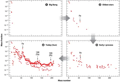
1.1 Chemical enrichment of the Universe, from Wiescher et al. (2012) 3

2.1 Theoretical HK tracks . . . 20

2.2 Theoretical HK tracks using SkyMapper v . . . 21

2.3 Ca ii filter transmission . . . 23

2.4 Positions of the fields observed within the LMC. . . 25

2.5 DDO51 filter foreground star rejection . . . 30

2.6 Fitting the HK colour-colour plot . . . 32

2.7 Example of region selection effects on region fit . . . 33

2.8 HK diagram with metal-poor isochrones . . . 34

2.9 HK residuals with metal-poor isochrones . . . 35

2.10 Cole et al. (2005) stars overlaid on HK diagram and CMD of LMC26 37 2.11 Location of HE0107 on the HK diagram and in the CMD . . . 39

2.12 Location of HE0305 on the HK diagram and in the CMD . . . 40

2.13 Location of HE0557 on the HK diagram and in the CMD . . . 41

(9)

2.15 HK diagram and CMD for 47 Tuc . . . 43

2.16 Example CMD and HK diagram for LMC field 26 . . . 46

2.20 CMD and HK diagram for LMC field 15 . . . 50

3.1 Example fibre allocation for an AAOmega + 2dF field . . . 59

3.2 Velocity of measured stars in the LMC by position . . . 63

3.3 Observed lines in IR spectra at different metallicities . . . 67

3.4 Velocities of the Cole et al. (2005) stars . . . 70

3.5 Metallicities of the Cole et al. (2005) stars . . . 71

3.6 Potential NGC1939 candidate spectra . . . 76

3.7 Example spectra from CTIO stars . . . 78

3.8 Distribution of metallicity in our sample . . . 79

4.1 Efficiency of HK candidate selection . . . 82

4.2 HK index vs measured metallicity . . . 83

4.3 Spectrally identified metal-poor stars on the CMD . . . 84

(10)

4.5 Example false-positive spectra for HK index . . . 86

4.6 Inner LMC field metallicity distributions . . . 88

4.7 Outer LMC field metallicity distributions . . . 89

4.8 Velocity distribution of metal-poor stars . . . 90

4.9 Potential EMP LMC star . . . 94

4.10 Second most metal-poor star in our sample . . . 96

A.1 Fit to the data with included background galaxies for LMC field 15 101 A.2 Fit to the data with included background galaxies for LMC field 13 102 A.3 Fit to the data with included background galaxies for LMC field 11 103 A.4 Fit to the data with included background galaxies for LMC field 8 104 A.5 Example HK residual diagram for LMC field 26 . . . 105

A.6 Example HK residual diagram for LMC field 25 . . . 106

A.9 HK residual diagram for LMC field 15 . . . 109

(11)

B.1 LMC field 26, observation 1 spectra. Part 1 . . . 125

B.17 LMC field 24 spectra. Part 1 . . . 141

(12)

B.22 LMC field 13 spectra . . . 146

B.23 LMC field 11 spectra . . . 147

(13)

1.1 Metal-poor star nomenclature . . . 5

1.2 Age and metallicity tracers in the LMC . . . 15

2.1 Photometric calibration fields . . . 26

2.2 The number of candidate stars identified in fields . . . 54

3.1 AAOmega +2dF target allocation priorities for observation . . . . 57

3.2 Known metal-poor objects observed at AAO . . . 60

3.3 Metal-poor calibrator equivalent widths . . . 66

3.4 Velocities for Cole et al. (2005) stars . . . 72

3.5 Equivalent width calculated metallicity for Cole et al. (2005) stars 73 3.6 NGC 1939 observations . . . 75

4.1 VMP star list . . . 91

4.2 VMP star list, continued . . . 92

4.3 Potential EMP stars in the LMC . . . 95

(14)

A.1 Summary observation log for CTIO data. . . 98

A.2 Summary observation log for CTIO data - continued. . . 99

A.3 Summary observation log for CTIO data - continued. . . 100

B.1 Stars with řEW ă4 in LMC field 26 - observation 1. . . 117

B.2 Stars with ř EW ă4 in LMC field 26 - observation 2. . . 117

B.4 Stars with ř EW ă4 in LMC field 25 - observation 1. . . 119

B.6 Stars with ř EW ă4 in LMC field 24. . . 121

B.7 Stars with řEW ă4 in LMC field 20. . . 122

B.8 Stars with ř EW ă4 in LMC field 15. . . 122

B.9 Stars with řEW ă4 in LMC field 13. . . 123

B.10 Stars withř EW ă5.5 in LMC field 11. . . 123

(15)

Introduction

All matter in the universe started out as a combination of the light elements

hydrogen, helium, and minute amounts of lithium that were produced in the Big

Bang. As stars aged, they began to create heavier elements - carbon, nitrogen,

oxygen, silicon, increasing in atomic number up to iron, dependent on their mass.

The production of these elements produces energy for the stars, but the formation

of elements heavier than iron results in a net loss of energy. The energy to form

heavier elements is provided in abundance during the final stages of massive stars’

lives. Stars more massive than „ 8 Md end their lives in explosive supernova

events (type II supernova), which are responsible for the creation of elements up

to uranium (Pagel 1997). These supernovae expel all these elements, dispersing

them into the interstellar medium, where they are incorporated into the next

generation of stars.

The next generation of stars has the remnants of the previous generation, and

therefore is slightly more metal-rich1 _{than its predecessors. Eventually, some of}

these stars will also go supernova, contributing the remnants of its predecessors

1_{Metal refers to any elements other than hydrogen and helium.}

(16)

and the metals they created during their lives to the interstellar medium. This

process is known as the chemical enrichment of galaxies.

The most recent stars to form in our Galaxy contain the elements produced by

several generations of stars before them. These stars are metal-rich and are

gener-ally found in areas of recent star-formation. In the Milky Way (MW), these stars

are primarily found within the disk. The older stars in a galaxy have not had

the continual enrichment of the young stars and hence are typically metal-poor

by comparison. These stars are typically located in the halo and the thick disk

of galaxies like the MW. This leads to an observable anti-correlation between age

and metallicity, the age-metallicity relation (AMR).

The distinction between the young and old stars of galaxies led to the definition

of stellar populations. The younger, visibly bluer stars were called Population

I, as they stood out from the redder, older stars, which were called Population

II. These two populations also shared a distinction in their metallicities due to

the nature of chemical evolution (e.g. Wiescher et al. (2012)). Therefore, the

metallicity of the Population II stars can be used to infer the duration of major

early star-forming activity in their host galaxy. The way abundances of elements

change with time is shown in Figure 1.1.

Population II have only had metal contributions from a few progenitor stars, with

the most metal-poor Population II stars only having contributions from one or two

supernovae. The progenitors of the most metal-poor stars would have formed with

effectively zero metal content, containing only the first elements created during

the Big Bang (Bromm 2013). These stars represent an as yet unobserved third

population of stars, called Population III. Population III stars are responsible

for the reionisation of the early Universe and the energy of their stellar winds

(17)

[image:17.612.140.528.256.521.2]

(18)

strongly shaped the early evolution of galaxies. If any of these Population III

stars exist today, they will be invaluable in contributing to our knowledge of the

early Universe.

1.1 Metal-Poor Stars

Metal-poor stars are among some of the oldest members of a given stellar

popula-tion. Due to their usefulness as probes for the early epochs of galaxy formation,

they have been the subject of many surveys over the last several decades, e.g.

Bond (1970), Beers et al. (1985), Frebel et al. (2010), and Starkenburg et al.

(2017). However, these metal-poor stars have remained relatively scarce, as they

have proven difficult to identify, e.g. as in Christlieb et al. (2002).

The degree to which a star is metal-poor can be determined by measuring the total

metal abundance [M/H] within that star. A proxy for the total metal abundance

is [Fe/H], the abundance of iron in the star with respect to the Sun, given in

equation 1.1.

rFe{Hs “log10

ˆ

NF e NH

˙

´log10

ˆ

NF e NH

˙

d

(1.1)

The term metal-poor refers to a large range of metallicities, typically anything

below [Fe/H]“ ´1.0. To avoid ambiguity, we will adopt the nomenclature defined

in Beers & Christlieb (2005) for classifying levels of metal deficiency, given in Table

(19)

Table 1.1: The nomenclature for metal-poor stars as suggested by Beers & Christlieb (2005)

[Fe/H] Term Acronym

ă ´1.0 Metal-Poor MP

ă ´2.0 Very Metal-Poor VMP

ă ´3.0 Extremely Metal-Poor EMP

ă ´4.0 Ultra Metal-Poor UMP

ă ´5.0 Hyper Metal-Poor HMP

ă ´6.0 Mega Metal-Poor MMP

Many different methods have been used in attempts to identify these metal-poor

stars in the field, primarily within the MW. The earliest metal-poor stars were

linked to the halo of the MW, and as such, the surveys pre-selected stars based

on their proper motions. Such studies are very limited, as they are restricted

by the metallicity distribution function (MDF) of the populations in which they

reside, and are kinematically biased, as there are many metal-poor stars without

high proper-motions (Bond 1970; Beers & Christlieb 2005). Attempts to identify

kinematically unbiased populations thus required a different methodology for

se-lection of stars - for which we have two potential applicable wide-scale options:

objective-prism based spectroscopic surveys, and colorimetric surveys (Christlieb

2006).

The survey by Bond (1970) was one of the first spectroscopic surveys to specifically

search for metal-poor stars in the galaxy, covering 4000 square degrees of the

MW. This survey was the first to indicate the extent of proper motions that

metal-poor stars had, and show that metal-poor stars weren’t limited to having

(20)

of known metal-poor stars with Mv ă `2.0 and [Fe/H]ď ´1.5 by 132 stars. The

lowest metallicity stars observed in these first surveys were around [Fe/H]“ ´3.0,

leading to the conclusion that stars of greater metal deficiency were exceedingly

rare.

A majority of known VMP stars were discovered by the HK survey by Beers et al.

(1985) and Beers et al. (1992), and the Hamburg/ESO (HES) survey (Christlieb

et al. 2002). Both surveys are objective-prism-based, covering a large area of the

MW,„2000 square degrees for the HK survey, and„5000 for HES. The selection

of apparently poor spectra yielded approximately 1000 stars more

metal-poor that [Fe/H] “ ´2.0, and „100 stars more metal-poor than [Fe/H] “ ´3.0,

increasing the number of known EMP stars by a factor of 7. These candidate

stars were selected based on the widths of the Ca ii K line and the Balmer lines

in their spectra. Due to a limiting magnitude of V ď15.0, a majority of the stars

discovered in this survey were relatively close, having distances between 2 kpc

and 10 kpc. In addition, the HK survey was the first to identify objects in the

UMP category (Beers et al. 1992).

Both spectroscopic and colorimetric methods are effective at identifying candidate

metal-poor stars in wide fields, but still require confirmation of metallicity using

follow-up medium-to-high-resolution spectroscopy. Spectroscopic surveys are

ca-pable of efficiently identifying metal-poor stars within the MW, and as such, these

types of survey have been the most effective, yielding a majority of the known

VMP stars in our galaxy to date.

Objective-prism-based spectroscopic surveys become increasingly difficult in the

more crowded fields due to overlapping spectra, thus they tend to be limited to

higher Galactic latitudes. For the more crowded fields, colorimetric surveys are

(21)

colours of the stars. The sensitivity to changes in metallicity is dependent on the

photometric filter system used in the survey (Beers & Christlieb 2005). Additional

filters can complement standard filter systems, enhancing the capacity to detect

lower metallicity stars. For example, a narrowband filter centred on the region

around the CaiiH & K lines, when used in conjunction with theuvby filters, could

distinguish metallicities down to [Fe/H] “ ´3.4 (Anthony-Twarog & Twarog

1998).

Recently, there have been several photometry-based surveys searching for

metal-poor stars, such as SkyMapper (Schmidt et al. 2005; Keller et al. 2012) and

PRISTINE (Starkenburg et al. 2017). Both of these surveys rely on the use of a

filter sensitive to changes in the Ca ii H & K lines to detect metal-poor objects.

SkyMapper observed the entire southern sky, with survey limits similar to the

Sloan Digital Sky Survey. This survey has been responsible for the discovery of

122 previously unknown stars, 41 of which were confirmed to be EMP.

SkyMap-per is the first program to observe stars in the MMP category (eg. Nordlander

et al. (2017); Keller et al. (2014)), which puts their metal content close to the

elusive population III stars. PRISTINE also showed high efficacy in the

selec-tion of metal-poor targets based on their photometry, with a reported successful

identification rate of 70 percent for stars more metal-poor than [Fe/H] “ ´2.5

(Youakim et al. 2017), identifying 33 new EMP stars.

Such low numbers of reported EMP stars in these surveys are a result of the MDF

of the galaxy. In a given population, the chances of observing a metal-poor star

decreases by a factor of 10 for every factor of 10 decrease in metallicity. It is

estimated that EMP stars represent a proportion of fewer than 1 in 1000 stars

(Norris 2004). Due to the scarcity of the lower metallicity stars, this relationship

isn’t well defined below [Fe/H] “ ´3.0. Results indicate that as few as 1 in

(22)

(Christlieb 2006).

There is a hypothetical lower limit to the metallicities of stars that have active

interiors. Mixing within a star that formed with very low metal content (e.g.

Population III stars) would have a metallicity of [Fe/H]« ´5.7 today (Iben 1983).

Currently, only one star has been discovered below this limit with a metallicity

of [Fe/H] ď ´6.5 (Nordlander et al. 2017; Keller et al. 2014).

1.1.1 The Importance of Metal-Poor Stars

The study of metal-poor stars can provide key insights into several aspects of

galaxy formation and the early epochs of the universe. They can be used to

test the IMF of high-mass stars, the earliest chemical evolution of galaxies, and

supernova yields. Due to the scarcity of the HMP and more metal-poor stars,

this parameter space is not well understood.

The initial element abundances of the universe are not directly measurable.

Metal-poor stars hold information on the chemical enrichment that occurred prior to

their formation, which can be used to model the production of elements in the

early universe. There are several different methods by which stars form their

elements, from alpha elements created in helium burning stars, to the iron peak

elements found in the cores of massive stars, to s- and r- process neutron-capture

elements. The heavier elements that are produced during explosive supernovae

are one of the better tracers of the predecessor population of stars.

The r- and s- processes are neutron capture mechanisms that allow for the

forma-tion of heavy elements. The r- process (rapid) produces heavy elements through

the rapid capture of neutrons and subsequent β´ _{decay. This process requires a}

(23)

core-collapse supernovae (Meyer 1994). The s- process (slow) allows for decays of the

nucleus between neutron captures, and requires far less extreme environments

when compared to the r- process. The s- process elements primarily form in AGB

stars during helium burning phases (Meyer 1994).

In the most ancient metal-poor stars, very little chemical enrichment occurred

prior to their formation. The chemical enrichment in these particular stars is

primarily from the supernovae (SNe) of the preceding stellar populations mixing

with the interstellar medium. At most, only a few SNe contributed to the heavy

element content of the most metal-poor stars (McWilliam et al. 1995; Keller et al.

2014). By comparison to models that predict the heavy elements produced during

SNe, the abundance patterns in these stars can indicate the conditions under

which the progenitor stars created and distributed heavy elements (Shigeyama

et al. 2000).

The ability to determine the early metal formation (specifically r- and s-process

elements) rates is particularly useful in modelling supernova element production

and testing the very end stages of a star’s lifecycle. Aoki et al. (2013) tested

models’ ability to reproduce element abundance trends seen in metal-poor stars

and found that the element abundance trends within EMP stars were indicative

of a ‘truncated r-process’, in which the progenitor star initially forms as a neutron

star, and then collapses through accretion to form a black hole. Observations of

metal-poor stars by Yong et al. (2013a) suggest that there are an additional two

methods by which heavy elements are formed other than the r-process.

Although metal-poor stars are classified as such through their relative lack of

(24)

to iron2. For many elements, [X/Fe] is relatively constant for a majority of a

star’s life, barring any external contribution. Each nucleosynthetic process that

occurs in a star will contribute to the enrichment of only a few elements. The

[X/Fe] abundance trends in metal-poor stars can be useful in testing the processes

that formed those elements (e.g. Spite et al. (2018)). The measurement of these

abundances is particularly useful for elements that are commonly associated with

high energy events like supernovae.

Several neutron-capture elements show consistent overabundances in metal-poor

stars. The measured abundances of barium and europium are key indicators of

neutron capture production, with the value of [Ba/Eu] changing dramatically

be-tween stars that formed elements under s-process and those that formed elements

under r-process (Beers & Christlieb 2005). The variation in abundance patterns

in metal-poor stars has indicated that if r-process elements are overabundant,

then the stars were likely produced by low mass type-II supernovae (McWilliam

et al. 1995).

The abundance of these r-process elements can determine the age of the star,

in particular, thorium and uranium. Finding metal-poor stars with measurable

r-process elements can help constrain the ages of the stellar populations to which

these metal-poor stars belong, as they are some of the oldest stars in those

pop-ulations (Sneden et al. 2001).

Approximately 20% of stars with [Fe/H]ă ´2.0 have an overabundance of carbon

(Rossi et al. 2005), with a similar fraction below [Fe/H] ă ´3.0 (Yong et al.

2013b). Given this trend is frequent in the metal-poor star population, under the

nomenclature of Beers & Christlieb (2005), any star with carbon overabundances

2_{The abundance ratio is represented by [X/Fe], where X represents any element other than}

(25)

of [C/Fe] ą `1.0 is termed a carbon-enhanced metal-poor (CEMP) star3.

Due to the small number of HMP- class stars currently known, the abundance

ratios of other elements at the low metallicity scale are not determined. Only

a few stars are currently known with metallicities below [Fe/H] “ ´5.0, two of

which have metallicities of [Fe/H] “ ´5.3 (Christlieb et al. 2004a), and [Fe/H]

“ ´5.4 (Frebel et al. 2005). Both of these stars are CEMP stars, having large

overabundances of carbon, with [C/Fe] « `4.0. In the most metal-poor star

currently known, with an estimated metallicity of [Fe/H] ď ´6.53 (Nordlander

et al. 2017), the abundance trends indicate that the star appears to have been

enriched by at most only a few low-energy supernovae (Keller et al. 2014).

To understand galaxy formation, knowledge of the distribution of masses of the

first stars is important. This mass distribution is known as the initial mass

function (IMF) and represents the range of masses over which stars enter the

main sequence. Metal-poor stars play an important role in constraining the IMF

at low metallicities. Indeed, studies suggest that the IMF of galaxies is skewed,

with a majority of the early stars having high masses, and any low-mass stars

potentially forming as binaries (Tumlinson 2007b). The link between CEMP

stars and the extremes of the metallicity scale are linked to the IMF by how these

low-mass stars are able to form. There is a threshold of C and O required to

form low-mass stars in the early Universe, as these elements provide a cooling

mechanism for the gases to form low-mass stars (Bromm 2013). Therefore, any

stars extremely low in metallicity at low mass must have formed from a gas above

these critical thresholds of [C/H] “ ´3.5 and [O/H] “ ´3.0.

The low-mass end of the IMF can be used to understand the way in which the

cos-mic cos-microwave background (CMB) has changed with time. As the CMB changes,

(26)

the minimum temperature of gases also changes. Metallicity affects the

temper-atures at which stars can form from gas (through cooling), hence the IMF would

change as the CMB changes. Using the results from Abel et al. (2002) and Bromm

et al. (2002), Tumlinson (2007a) showed that there was a relation between the

CMB and the IMF and found indications that the CMB has an effect on the

masses of stars formed early in the Galaxy.

Another of the important characteristics of a galaxy to understand is the

pro-portion of stars that exist at given metallicities, described by the MDF. The

MDF can be used to test the ability of stellar formation models to replicate

ob-served trends. The MDF can also provide estimates for the proportion of peculiar

metal-poor stars (such as CEMPs) (Yong et al. 2013b). Because stars become

increasingly scarce at lower metallicities, the low metallicity end of the MDF is

not well understood.

Understanding the way in which the most metal-poor stars (UMP and HMP)

received their metal enrichment provides information about the Population III

stars - the first stars that formed in their galaxy. The observations of these UMP

and HMP stars can help constrain the MDF of Population III stars, and the star

formation rate when Population II stars were beginning to form (Rollinde et al.

2009).

There is a wealth of knowledge that can be gained from studying metal-poor stars,

and as such, the discovery of new metal-poor stars is important. Unfortunately,

metal-poor stars become increasingly rare as metallicity decreases, with only a

handful existing in the HMP category. Filling this parameter space will be

in-valuable for testing the conclusions based on the small number of these presently

(27)

1.2 The Large Magellanic Cloud

There have been extensive studies looking for metal-poor stars in the Milky Way

and its metal-poor satellites. The dwarf spheroidal galaxies Fornax, Sculptor and

Sextans have confirmed EMP stars resulting from the surveys of these satellites

(Tafelmeyer et al. 2010). However, there hasn’t been much work on our nearest

significant mass neighbour, which we have reason to believe would be an excellent

place to search for EMP stars.

The Large Magellanic Cloud (LMC) is one of the Milky Way’s satellite galaxies.

With a mass of between M = 1010_M

dand M = 1011Md(van der Marel et al. 2002;

Laporte et al. 2018) (between 1% and 10% of the Milky Way’s mass), it is classified

as a barred late-type spiral. The galaxy formed approximately 13 Gyr ago and

had formed about half of its stars between 5 and 7 Gyr ago (Weisz et al. 2013).

Observation of the LMC is relatively easy, as we view it from almost directly

face-on. Studies of the LMC are important as they provide comparisons for Galactic

formation models, and help in understanding galaxies with companions such as

our own (Robotham et al. 2012).

The distance to the LMC is now well determined by Pietrzy´nski et al. (2013),

who used eclipsing binary systems to constrain the distance to approximately

2%. The LMC distance was determined to be dLM C “ 49.96˘1.11 kpc. The

proximity of the LMC has allowed for a great number of studies into its evolution

and composition, and as such, is one of the Milky Way’s most studied satellite

galaxies.

Tidal interactions between the LMC and the Milky Way, and between the LMC

and Small Magellanic Cloud (SMC) have both played a part in the star formation

(28)

et al. 2013). An interaction between the LMC and the MW appears to have

occurred approximately 3-5 Gyr ago, which is around the time when the LMC

bar formed (Cole et al. 2005), corresponding to a burst in SMC star formation

(Cignoni et al. 2012). The LMC-SMC system had its closest approach with the

MW approximately 1 Gyr ago, and the LMC - SMC system has an orbital period

of „ 1 Gyr, with the most recent interaction between 150 Myr and 200 Myr ago

(Kallivayalil et al. 2013).

For recent star formation events in the LMC (i.e. over the past„2 Gyr, starting

about 3 Gyr ago), there are observed coincident events in the SMC, further

sup-porting interaction-induced star formation (Harris & Zaritsky 2009; Weisz et al.

2013). Although there has been star formation throughout the history of the

LMC, the star formation rate between 12 and 5 Gyr was relatively quiescent, a

trend that is shared by the SMC (Weisz et al. 2013).

The quiescent period of star formation is accompanied by a lack of globular cluster

formation. Nearly all of the globular clusters observed in the LMC were formed

around 13 Gyr ago, or in the past 3 Gyr, with only one cluster observed of

intermediate age (Da Costa 1991). The formation of new clusters 3 Gyr ago

coincides with a peak in the SFR, possibly due to an LMC-SMC interaction.

The cluster age gap is of interest because the cluster and field star populations

share a similar age-metallicity relationship (AMR), with the field star formation

continuing during the age gap (Geha et al. 1998). By comparison, the SMC

has a distribution of cluster ages extending back to its oldest clusters (Da Costa

1991). The cluster population is analogous to the Milky Way’s cluster population

(Harris & Zaritsky 2009) (with the exception of the cluster age gap), with the

notable exception of massive young clusters that have formed as a result of the

(29)

The AMR of various populations within the LMC have been studied by several

authors (e.g. Cole et al. (2005); Carrera et al. (2011); Piatti et al. (2012)). Based

on the AMR derived from red giant stars in the central bar, Cole et al. (2005)

noted a lack of chemical evolution during the cluster age gap (i.e. the AMR was

flat during this epoch). From the study of Cole et al. (2005), the majority of red

giants in the bar have mean metallicity [Fe/H] “ ´0.4, with a distribution

ex-tending down past [Fe/H]ă ´2.0. Piatti et al. (2012) used wide-field Washington

photometry covering a majority of the galaxy with the purpose of establishing an

AMR (Piatti & Geisler 2013). The results of Piatti & Geisler (2013) found that

the cluster AMR at the ancient ages acted as a lower limit to the field population

AMR. There are indications that the initial chemical enrichment rate was quite

steep, reaching a value of [Fe/H] “ ´1.0 within the first 2-3 Gyr (Carrera et al.

2011). A list of common age and metallicity tracers is given in Table 1.2.

Table 1.2: A few of the metallicity and age tracers in the LMC, given is the mean

metallicity of these populations.

Tracer Metallicity Age Refsa

[Fe/H] Gyr

Young Globular Clusters ´0.4 ă2.5 Gyr Piatti et al. (2018a)

RR Lyrae ´1.5 ą10 Gyr Haschke et al. (2012)

Old Red Giants ´0.4 ą10 Gyr Cole et al. (2005)

a _{Example references for the values given in this table.}

From the trends of alpha elements observed in the LMC, it is likely that the

primary source of chemical enrichment is from type Ia supernovae4 _{(Van der}

4_{Type Ia supernovae are caused by accretion onto white dwarf stars from a binary partner,}

(30)

Swaelmen et al. 2012b). The domination of enrichment from type Ia supernovae

occurs at lower metallicities than is seen to occur in the Milky Way (Van der

Swaelmen et al. 2012a). Through an analysis of the chemical enrichment history

of the LMC, Van der Swaelmen et al. (2013) concluded that massive stars had

less of a contribution to the total enrichment of the galaxy than they do in the

Milky Way. Also observed in the study of Van der Swaelmen et al. (2013) was a

difference in abundance patterns for the disk and bar stars.

1.2.1 Metal-Poor Stars in the LMC

There have been very few studies focussing on finding individual metal-poor stars

within the LMC. Currently, there are only a handful of stars known with

metallic-ity [Fe/H] ă ´2.0 (Cole et al. 2005; Carrera et al. 2011; Van der Swaelmen et al.

2013). Measurements of RR Lyrae stars have yielded one of the lowest

metallic-ity objects known in the LMC (albeit with some degree of uncertainty due to the

faintness and variability of the star), with reported [Fe/H] “ ´2.7 (Haschke et al.

2012).

Beyond these few examples, there have been no large attempts to delve into the

metal-poor side of the MDF beyond [Fe/H] “ ´2.0. Many wide-scale surveys

are performed in broadband systems, which have little sensitivity to changes in

metallicity below this threshold. If the relationship between the metallicity and

the frequency of metal-poor stars as described in Norris (2004) holds true in the

LMC, then we can make a guess at the frequency of EMP class stars among the

LMC’s giant population. Given the distribution of red giant stars in the LMC as

(31)

stars to be classed as EMP or more metal-poor5.

The low line of sight reddening and the well-determined distance make the LMC

a suitable place to search for EMP stars, as we can see down to the centre of

the galaxy from the outside, unlike our views into the MW bulge. These central

regions are likely to have the greatest proportion of metal-poor stars, due to their

distribution (Tumlinson 2010).

It is not well known if the low metallicity scale of the LMC reflects what is seen in

the MW. From this project, we expect to expand the lowest region of the MDF,

probing below [Fe/H] “ ´2.0 to fill in this parameter space for the LMC.

5_{Assume the frequency of poor stars follows a power-law distribution when the}

metal-licity is less than [Fe/H]ď ´0.7, which in Cole et al. (2005), accounted for 10% of the red giant population. Then, for a star with at least [Fe/H]“ ´3.0, we have

0.10

ş´0.7

´8 10 x_dx

ż´3

´8

10xdx«0.0005

(32)

Photometric Survey

This study takes inspiration from Anthony-Twarog & Twarog (1998), wherein

the use of a narrowband filter in combination with the broadband Str¨omgren

uvby filter system was shown to be a good tracer of metallicity, showing good

metallicity sensitivity and a low false positive rate as confirmed with spectroscopy

(Anthony-Twarog et al. 2000).

Broadband photometric colours begin to lose sensitivity to changes in metallicity

around [Fe/H] “ ´2.0. The Washington CMT1T2 filter system was designed to

provide better temperature and metal abundances for G & K giant stars (Canterna

1976). This photometric system has been proven to be a good metallicity indicator

when compared to other photometric systems, achieving some results down to a

metallicity of [Fe/H] « ´2.5 (Geisler et al. 1991).

Instead of the Str¨omgren filters, we are using the Washington C & M filters

with Cousins R & I as substitutes for Washington T1 & T2 (Geisler 1996). In a

fashion similar to Anthony-Twarog & Twarog (1998), we establish an index for

the differentiation of metallicity. We will define our measure as the HK index:

(33)

HK“ pCaii´Mq ´ pM´Rq (2.1)

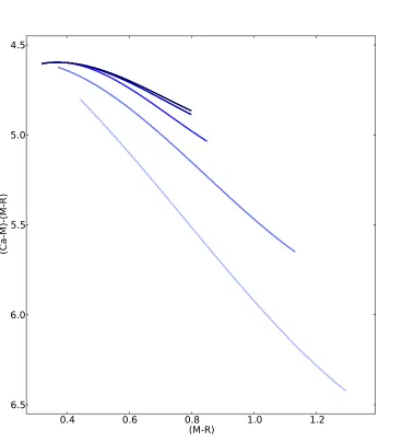
We show the ability of this HK index to differentiate metallicities below [Fe/H]“

´3.0 in Figure 2.1. The Washington and Cousins filter predictions were obtained

from MIST isochrone grids (Dotter 2016; Choi et al. 2016; Paxton et al. 2011, 2013,

2015), and the calcium filter data were acquired from ATLAS model atmosphere

grids (Kurucz 1970). The calcium filter magnitude was estimated by interpolating

between grid values at the given metallicities for the corresponding MIST Tef f

and log g.

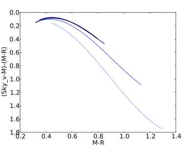
To demonstrate the increase in the sensitivity of a photometric system paired

with a narrowband filter, we compare Figure 2.1 to Figure 2.2. In Figure 2.2,

we have taken the SkyMapper v filter as a representative calcium filter, and have

constructed the HK index as in equation 2.1 using MIST isochrone grids. The

SkyMapper v filter has a central wavelength of λ “ 384nm with ∆λ “ 28 nm

(Bessell et al. 2011), which is slightly bluer and wider than the one used in this

study. From this figure, we see that using a wider filter can result in a loss of

sensitivity1 _{below [Fe/H]}

“ ´3.0.

1_{SkyMapper uses a different metric to determine metallicity in their surveys. This example}

(34)

0.4

0.6

0.8 _(M-R)

1.0

1.2

4.5

5.0

5.5

6.0

6.5

[image:34.612.155.534.139.543.2]

(Ca-M)-(M-R)

Figure 2.1: HK index against (M-R) colour using MIST isochrones with Kurucz model

atmospheres to estimate the Ca ii filter magnitudes. The tracks have metallicities of

(35)

0.2

0.4

0.6

0.8

1.0

1.2

1.4 M-R

0.0

0.2

0.4

0.6

0.8

1.0

1.2

1.4

1.6

1.8

[image:35.612.138.538.134.436.2]

(Sky_v-M)-(M-R)

Figure 2.2: Skymapperv HK index against (M-R) colour using MIST isochrones. The

tracks have metallicities of [Fe/H] “ ´1.0,´2.0,´3.0,´4.0,and ´5.0, from lightest to darkest, respectively. All isochrones have an age of 13 Gyr. In this example, the isochrones become degenerate at [Fe/H] “ ´3.0.

2.1 Observations

The photometric data were taken by Andrew Cole and Doug Geisler during the

nights of the 27th to the 31st of December 2008 with the 4-m Blanco telescope at

the Cerro Tololo Inter-American Observatory (CTIO) using the MOSAIC-II CCD

imager. The MOSAIC-II detector consists of eight 2048ˆ2048 pixel SITe CCDs,

(36)

over the four nights, each covering an area of 361

ˆ361_{, for a total observational}

area of 5.4 square degrees. The seeing for the observations varied between 0.6”

and 1.7”, with a typical value of „ 1”. Airmass varied between „ 1.1 and 1.7.

In addition to these observations, partial data2 _{for some of the science fields}

were obtained a week prior (on the 21st of December) by Doug Geisler. These

additional observations were combined with the primary data in the analysis.

In addition to the C, M, R & I filters, the fields were also observed with the DDO51

filter, which is centred on the Mgb and MgH lines at λ„515nm. This filter can

be used in conjunction with our M and I filters to help screen for unwanted

foreground contaminants (Majewski et al. 2000) based on surface gravity.

The sixth filter used to observe our fields is a custom-built narrowband filter,

centred on the Caii H & K lines. The filter was manufactured by Omega Optical

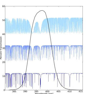
with a central wavelength ofλ“396.5˘2nm, and a FWHM of 9˘2nm. The filter

was specified to have a transmissivity of at least 50% at the central wavelength.

The measured bandpass of the filter is shown in Figure 2.3 with some example

spectra at different metallicities, showing the change in the H & K lines as the

metal content decreases.

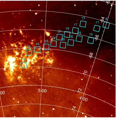
The science fields were aligned along the bar of the LMC, in the direction of

the greatest falloff in stellar density, shown in Figure 2.4. The innermost field

covers the same region observed in Cole et al. (2005), which we will use as a

metallicity calibration between [Fe/H] “ ´0.4 and ´2.0 for our data. This field

also contains the metal-poor globular cluster NGC1939, which has a metallicity

of [Fe/H]“ ´2.10˘0.19 (Mackey & Gilmore 2004). In the inner fields, we expect

a stellar density of „ 1000 red giant branch (RGB) stars per square degree,

decreasing to only „ 20 RGB stars per square degree in the outermost field

(37)

385

390

395

400

405

410

415 Wavelength (nm)

0

10

20

30

40

50

60

[image:37.612.158.537.179.566.2]

Percent Transmission

Figure 2.3: The transmissivity of the Omega Optical Ca ii filter superimposed over

POLLUX synthetic spectra (Palacios et al. 2010). The spectra have [Fe/H] “1.0, 2.5, and 4.0, and Tef f “5000, 5250, and 5500 from top to bottom, respectively. All three

(38)

(Nikolaev & Weinberg 2000).

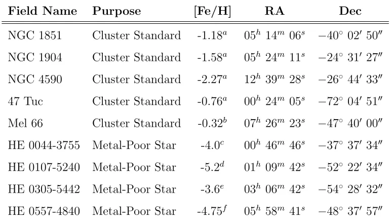
For each night, a selection of calibration sources was observed, listed in Table

2.1, with the full list of observations given in Tables A.1 to A.3. The standard

star fields PG0321, SA 98, SA 101, and NGC 3680 are the standard fields from

Geisler (1996) and are used to calibrate the photometric system. The metal-poor

star fields were offset from the star of interest by 21 _{N and 2}1 _{E, to ensure that}

the target wouldn’t land in the gap between chips. These metal-poor calibration

fields are useful for testing the candidate selection techniques detailed in section

2.2. The remaining cluster standard fields cover a range of metallicities between

(39)

[image:39.612.139.532.208.608.2]

11 13 15 16 17 18 8 21 23 20 25 22 24 19 26

4:00

5:00

6:00

-74

-72

-70

-68

-66

-64

-62

(40)

[image:40.612.141.526.160.378.2]

Table 2.1: Calibration fields observed at CTIO

Field Name Purpose [Fe/H] RA Dec

NGC 1851 Cluster Standard -1.18a ₀₅h ₁₄m ₀₆s

´40˝ 021 502

NGC 1904 Cluster Standard -1.58a ₀₅h ₂₄m ₁₁s _´₂₄˝ ₃₁1 ₂₇2

NGC 4590 Cluster Standard -2.27a ₁₂h ₃₉m ₂₈s

´26˝ 441 332

47 Tuc Cluster Standard -0.76a ₀₀h ₂₄m ₀₅s _´₇₂˝ ₀₄1 ₅₁2

Mel 66 Cluster Standard -0.32b ₀₇h ₂₆m ₂₃s

´47˝ 401 002

HE 0044-3755 Metal-Poor Star -4.0c ₀₀h ₄₆m ₄₆s _´₃₇˝ ₃₇1 ₃₄2

HE 0107-5240 Metal-Poor Star -5.2d ₀₁h ₀₉m ₄₂s

´52˝ 221 342

HE 0305-5442 Metal-Poor Star -3.6e ₀₃h ₀₆m ₄₂s _´₅₄˝ ₂₈1 ₃₂2

HE 0557-4840 Metal-Poor Star -4.75f ₀₅h ₅₈m ₄₁s

´48˝ 371 572

a _{Dalessandro et al. (2012)} b _{Netopil et al. (2016)} c _Fran¸_{cois et al. (2003)} d _{Christlieb et al. (2004b)} e _{Cayrel et al. (2004)} f _{Norris et al. (2007)}

2.2 Data Analysis

On each night, a set of bias, dark and flat field images was taken to perform

standard CCD basic calibration. All image reduction was done using the IRAF3

mosaic reduction package mscred. The 10 bias images from each night were

3_{IRAF is distributed by the National Optical Astronomy Observatory, which is operated}

(41)

averaged together, rejecting the minimum and maximum pixel values from the

image sets to account for cosmic ray interference. For each filter, 5 dome flats

were combined, rejecting pixels more than 3σ from the median level.

The sky flats were constructed using many non-crowded images, which were

aver-aged together rejecting pixels based on the readnoise and gain of the CCD, given

by: σ“ d ˆ RN Gain ˙2 ` xIy

Gain` psˆ xIyq

2

(2.2)

Where xIy is the pixel value, RN is the readnoise, and s is the sensitivity noise.

The range of acceptable values from the median is then calculated on a per-pixel

basis, with rejection occurring if the pixel value is below 5σ, or above 2.5σ.

The science frames then were corrected based on the bias and the dome flat fields

using the ccdproctask inmscred. These images were then processed once more,

applying the corrections from the sky flats. In this process,ccdprocautomatically

performs trimming of the overscan regions in the frame and corrects for any

crosstalk between CCD chips on the same amplifier.

Each amplifier was then merged in IRAF, and the multi-extension fits image split

into individual fits images for each amplifier for the following steps of the data

reduction.

The reduced data was then processed using the PHOTRED and STDRED

pack-ages, first described in Nidever et al. (2011). These IDL scripts make use of

Peter Stetson’s DAOPHOT and ALLFRAME packages (Stetson 1987, 1994) to

reduce crowded photometric fields. STDRED was used to calculate the

appro-priate transformation equations for each night’s data. PHOTRED was used to

(42)

fields4. PHOTRED was used to estimate the required aperture corrections for all

observed fields.

To ensure correctly combined images, these outer fields required processing in two

batches, ‘long’ exposures (C, Caii, and DDO51 filters), and ‘short’ exposures (I, R

and M filters). The results from these reductions were then combined by aligning

the frames using the stellar positions calculated by PHOTRED. There was a far

greater number of stars identified in the I, R, and M exposures, which could not

be included in the combined file, as the analysis required detections in four of the

six filters (I, R, M, and Ca ii).

The remaining fields were reduced by hand in DAOPHOT. The coordinates of

the stars in each filter were matched to the corresponding stars, using the I filter

as a reference. The positions of stars were allowed to vary by up to the average

PSF of the filter being matched. The resultant file was the best symmetric match

between the I filter and other filters, requiring matches in the above four filters. It

is worth noting that allowing the coordinates to vary will introduce some erroneous

matches.

The data were transformed to a standard photometric system using equations of

the following form:

R“Rinstć1ˆ pRinst Íinstq ć2ÂM ´R0ÀPR`2.5 log10tR (2.3)

Where c1 is the colour coefficient, c2 is the airmass coefficient, R0 is the

zero-point offset for filter R, APR is the aperture correction for filter R, and tR is the

exposure time. The colours used for the calibrations are (R-I) for Cousins R &

4_{Fields LMC20 and closer to the centre of the LMC suffered data quality issues in the output}

(43)

I, (C-M) for Washington C & M, and (Ca-C) for the Ca ii filter. The DDO51

filter did not have information in all of the standard fields that were observed,

so a reliable transformation equation could not be calculated using PHOTRED.

Any analyses following that use the DDO51 filter are thus utilising instrumental

values.

The data were then dereddened, using values from Schlegel et al. (1998) for I &

R, and O’Donnell (1994) for C & M. The reddening in the Caiifilter is calculated

using the same coefficient used for the C filter. The reddening towards the LMC is

relatively low, with E(B - V)«0.06 (from Schlegel et al. (1998)). While this value

will be appropriate for the outer fields, the inner fields have additional variation

from line-of-sight reddening within the LMC disk. The reddening in the inner

fields is still quite low, but can vary by up to E(B - V) « 0.1 (Haschke et al.

2011).

Because the LMC lies at a distance of 50 kpc, and the LMC is viewed nearly

face-on, we do not need to consider strong distance effects on individual stars

within a field. However, due to the distance, and the high degree of crowding in

our fields, we concentrate on the detection of RGB stars. To select these stars,

visual inspection of an I vs (R-I) colour-magnitude diagram (CMD) is used, and

constraints are placed on the data to analyse.

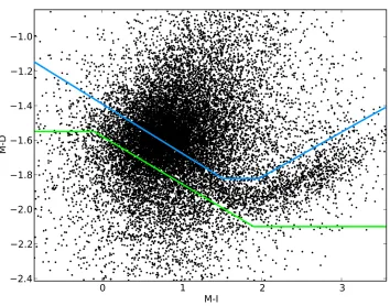
One issue to consider with this technique is the inclusion of MW foreground dwarf

stars, which will occupy a similar region in the CMD. Majewski et al. (2000)

detailed a method using Washington photometry in conjunction with DDO51 to

distinguish between stars with high surface gravity (main-sequence), and those

with low surface gravity (giant stars). We adopted this technique but allowed a

more relaxed cutoff range to allow for the large scatter in the data, rejecting only

(44)

an example of this in Figure 2.5, which contains all of the valid data5 from field

[image:44.612.148.502.198.476.2]

13.

Figure 2.5: Example colour-colour plot used to reject obvious foreground stars. The

blue line is approximately where the relation from Majewski et al. (2000) falls, which separates the giants (above the curve) from the dwarfs (below the curve). The green line is our rejection threshold, with any stars above this line being included in the candidate selection plots. Our rejection threshold is lowered to account for poorer quality photometry in the DDO51 filter. The ‘tail’ feature seen in this plot mainly consists of MW foreground objects, but may contain some number of RGB stars of interest.

Once the RGB stars are selected, they are plotted on the HK colour-colour plot.

(45)

Stars in this plot should occupy a narrow region on the diagram corresponding

to the age and metallicity of the mean of the LMC RGB population. Practically,

these stars will have some random errors associated with the photometry, and

some systematic errors associated with the reduction process. As the metal-poor

stars we are interested in are going to occupy specific areas in relation to the

main body of stars, we can greatly reduce the effects of the systematic errors by

looking at the positions of stars with respect to the population mean.

To look at the positions of stars with respect to the mean, we need to get an

idea of the mean stellar population. To do this, we define a region around the

densest population of stars and fit a third order polynomial to the data using

2-dimensional weighted least-squares. The third order polynomial was chosen

to mimic the general shape of the metal-poor stars in HK space without being

influenced too greatly by outliers. The results of doing this in our most densely

populated field are shown in Figure 2.6, in which we have defined the fit to the

(46)

0.0

0.5

1.0

1.5

2.0 (M-R)

4.0

4.5

5.0

5.5

6.0

6.5

7.0

7.5 (CaII-M)-(M-R)

LMC26 HK Index

Figure 2.6: Example HK Diagram showing fit to the region (in green) containing

the densest region of stars for a single amplifier LMC 26. The contour regions contain 93.75%, 87.5%, 75% and 50% of stars from lightest to darkest, respectively. Typical error bars for these data are given in the bottom-left.

We want to check that the selection of the region doesn’t greatly influence the

selection of candidate metal-poor stars, so we have shown an example of taking

a larger proportion of the stars in Figure 2.7. Over the range of colours we are

likely to find metal-poor stars, the difference between the two fits tends to be

small. The region selection only begins to have a large effect at the extremes in

(47)

(48)

0.0

0.5

1.0

1.5

2.0 (M-R)

4.0

4.5

5.0

5.5

6.0

6.5

7.0

7.5 (CaII-M)-(M-R)

LMC26 HK Index

Figure 2.8: HK from WISE isochrones and interpolated ATLAS model atmosphere

grids overlaid on the region shown in 2.6. Purple is an approximate typical LMC isochrone with Age“4 Gyr, [Fe/H]“ ´0.5; the blue isochrones begin at [Fe/H]“ ´1.0 and decrease in steps of 1 dex, to [Fe/H]“ ´4.0, with more metal-poor isochrones being darker. Contour levels are the same as in Figure 2.6

Using this technique, we can then measure the HK separation from the mean of

the population, giving us a rough idea of the metallicity compared to the rest of

the observed stars. Subtracting the fit from the data yields Figure 2.9, in which

we have included the isochrones from Figure 2.8. In this step, we also measure

the spread of the entire population (not just the region selected for the fit) to

categorise the stars. For our example (LMC26, amplifier 3), stars that had an

(49)

is the metric by which we identify our metal-poor candidates.

0.0

0.5

1.0

1.5

2.0 (M-R)

3

2

1

0

1

2 HK Residual

LMC26 HK Residuals

Figure 2.9: Residuals of HK diagram used to select metal-poor candidates, represented

with black diamonds. Isochrones are as in Figure 2.8; blue isochrones are 13 Gyr, [Fe/H]

“ ´2.0,´3.0, and´4.0, from lightest to darkest, respectively. The purple isochrone is a 4 Gyr, [Fe/H]“ ´0.5 isochrone. The dotted red lines represent the ˘2σ values of the HK values of all the stars in the plot. A typical error bar for the data is shown in the top-left.

The detection threshold was lowered for LMC20 to accommodate the lower

num-ber of stars in the field. For the outer fields, (fields with RA ă4h30m) both the I

magnitude and the detection threshold were lowered significantly due to the very

(50)

false positives, primarily foreground stars. These foreground stars are partially

screened as detailed above using the DDO51 filter.

Due to issues with the data quality and the reduction pipeline, only certain fields

were analysed. The science fields that were successfully reduced are LMC fields

8, 11, 13, 15, 20, 24, 25, and 26. Two of the clusters had usable data in some

filters - 47 Tucanae and NGC4590. Three of the four observed metal-poor stars

were also analysed: HE0107, HE0305, and HE0557.

2.3 Results

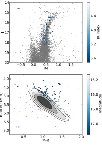
The most immediate test available to us is checking for consistency with the stars

already observed in Cole et al. (2005). We see that there is good agreement

be-tween typical RGB stars and the Cole stars, with some stars having HK indices

that could flag them as metal-poor under our selection criteria (Figure 2.10).

There are some stars with comparatively high scatter in the CMD and HK

dia-gram, which could indicate that there is some source of error in the photometry.

These errors could be caused by incorrect matching of stars between each of the

filters. Some level of mismatching is to be expected between filters due to the

high degree of crowding in the inner fields. This problem should only affect a

relatively small number of stars, which will diminish as we move further from

the central fields. It is reassuring that the CMD and colour-colour plots show

coherent, identifiable structures.

We also would like the metal-poor calibrators to be clearly identifiable in the HK

diagrams, as they are all on the extreme end of the metallicity scale. From Figures

2.11, 2.12 and 2.13, we see that the metal-poor objects are all located well above

(51)

(52)

10ăI ă18. There is a higher degree of scattering in the field containing HE0305

but the metal-poor star still lies „ 0.5 dex from the mean of the population,

about where we would expect metal-poor stars based off of the separation of the

isochrones from Figure 2.1.

The morphology of our HK diagrams can also serve as an indicator of any issues

that might be present in the data. For the inner fields6_{, a large percentage of}

the data is RGB stars, with some minor contribution from MW foreground dwarf

stars, and from MW asymptotic giant branch (AGB) stars. These foreground

objects occupy the same area of the HK diagram as the RGB stars. The ratio of

contaminants to genuine LMC stars increases dramatically as we move out from

the central regions. To lessen the impact of these contaminants, they are filtered

using the DDO51 Filter, as shown in Figure 2.5. A small number of obvious

foreground objects can be removed using this method, an example of which is

shown in Figure 2.14.

6_{LMC20 and inwards - those fields with RA}

(53)

0.5

0.0

0.5

1.0

1.5 R-I

12

14

16

18

20 I

0.0

0.5

1.0

1.5 M-R

4.0

4.5

5.0

5.5

6.0

6.5

7.0

7.5 (CaII-M)-(M-R)

Figure 2.11: Location of HE0107 (black diamond) in the HK diagram and the CMD of

(54)

0.5

0.0

0.5

1.0

1.5 R-I

12

14

16

18

20 I

0.0

0.5

1.0

1.5 M-R

3.5

4.0

4.5

5.0

5.5

6.0

6.5 (CaII-M)-(M-R)

(55)

0.5

0.0

0.5

1.0

1.5 R-I

12

14

16

18

20 I

0.2

0.4

0.6

0.8

1.0

1.2

1.4 M-R

4.5

5.0

5.5

6.0

6.5 (CaII-M)-(M-R)

(56)

Figure 2.14: Left: A CMD of all available LMC13 data after filtering with DDO51, as shown in Figure 2.5. Black points are all objects considered to be non-foreground objects, and red points are the objects returned by our metal-poor selection criteria. The filtering was only performed on objects with 0ă pR´Iq ă1.1, and 14ăI ă18.9.

Right: The approximate locations of features in the filtered region. These feature regions only indicate where we might expect to find a majority of the labelled objects.

The inclusion of other objects is apparent in the outer fields’ HK diagrams, in

which a second feature below the RGB stars begins to dominate. These objects

are most likely galaxies, having redder colours than the RGB stars. Ideally,

these objects are filtered out in the reduction process using DAOPHOT, with

the definition of the sharpness and roundness parameters allowing for rejection

of very obvious galaxies. These galaxy contaminants are probably more distant

(z ą1.5) elliptical galaxies, whose PSF is similar enough to typical stars to pass

the rejection criteria. There is also a minor spur feature in some of the diagrams,

most notably in the field of 47 Tucanae (Figure 2.15). This feature could result

from poor matches between filters in the photometric reduction step, caused by

the high degree of crowding in the images.

(57)

0.5

0.0

0.5

1.0

1.5 R-I

11

12

13

14

15

16

17 I

0.0

0.5

1.0

1.5 M-R

4.0

4.5

5.0

5.5

6.0

6.5

7.0

7.5 (CaII-M)-(M-R)

Figure 2.15: CMD and HK diagram for 47 Tucanae. Typical error bars for the data

(58)

fitting our data, as the fit is still very good in the region we expect to find

metal-poor stars (e.g. see Figures A.1 to A.4 in Appendix A). Due to the way in which

we select the metal-poor candidates, the inclusion of these galaxies could increase

the spread of HK index in the population, which we counteract by lowering the

detection threshold slightly.

In the determination of metal-poor candidates, we need to consider the effect that

reddening has on the HK index. From the reddening in the filters used to define

the HK index, the reddening in HK is given by:

AHK “0.234ˆEpB´Vq

Even if we expect at worst a variation of E(B - V) “0.1 among stars in a field7_,

the impact it will have on the HK index of the stars isă0.05 dex. Paired with the

effects of reddening on our temperature indicator, any stars with higher reddening

than what we have estimated will appear to be slightly more metal-rich in the HK

diagrams. These effects are much smaller than the errors from the photometry,

which are likely the limiting factor for the sensitivity of our technique.

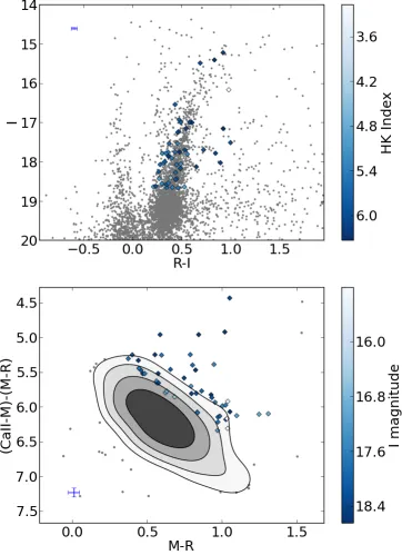
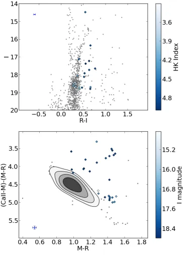
The following figures (2.16 to 2.23) show the locations of candidate objects in the

HK diagram, and in the I vs (R-I) CMD for the fields we analysed. Looking at

these diagrams, we can see that there is some zero-point issue between individual

fields, as the location of the bulk of stars in HK space is not consistent. This could

be a result of the crowding in the inner fields, as these are the fields in which the

effect is the most noticeable. Comparatively, the outer fields have a much more

consistent distribution of stars in HK space. As the candidates are calculated on

a per-amplifier basis, this is not going to impact the identification of metal-poor

stars.

In the fields with identifiable red giant branches, the candidates that are obviously

(59)

members of the RGB tend to lie on the blue side of the diagram. This is consistent

with our understanding of metal-poor stars.

From Tumlinson (2010), the oldest and most metal-poor stars of a galaxy are

most common on tightly-bound orbits in a galaxy’s halo. We expect to find a

majority of our metal-poor candidates in the inner fields of the LMC. In selecting

candidates for follow-up, we preferentially select from these inner fields.

Table 2.2 contains a summary of our candidate numbers for each field. These

objects were sorted based on their I magnitude to prepare for medium resolution

(60)

(61)

[image:61.612.145.504.93.604.2]

(62)

[image:62.612.143.505.97.596.2]

(63)

[image:63.612.141.505.94.601.2]

(64)

[image:64.612.158.490.95.594.2]

(65)

[image:65.612.157.494.95.592.2]

(66)

[image:66.612.159.495.94.589.2]

(67)

[image:67.612.157.494.95.592.2]

(68)

Table 2.2: The number of candidate stars identified in fields

Field Name Number of Candidates Notes

LMC26 1182 a

LMC25 553

LMC24 451

LMC20 81 b

LMC15 156 a,c,d,e

LMC13 210 a,c,d,e

LMC11 102 c,d,e

LMC8 173 a,c,d,e

a _{Some amplifier data were not included in the selection of candidates due to issues in}

the reduction process.

b _{The selection criterion was lowered to}_σ

ą1.2 due to a lower density of stars.

c _{The selection criterion was lowered to}_σ

ą0.7 due to the extremely sparse RGB population and the inclusion of background galaxies.

d _{More strict filtering based on surface gravity was used to constrain candidates in}

these fields.

e _{The cutoff for I magnitude was lowered in the selection criteria.}

The use of the HK index to select metal-poor candidate stars from a population

has proven successful in other surveys such as PRISTINE (Starkenburg et al.

2017), SkyMapper (Schmidt et al. 2005; Keller et al. 2012), and originally in

Anthony-Twarog & Twarog (1998). We have shown our HK index is capable of

resolving metal-poor stars from the remainder of the fields using known EMP

stars. Our choice of HK index is minimally influenced by reddening effects, which

(69)

There is a range of complicating factors in considering the use of our HK diagrams.

As our targets are very faint and crowded, a high degree of scatter in the central

fields is to be expected. Contributions to the HK index from chromospherically

active stars are also expected, something that cannot be easily distinguished solely

with photometry. Finally, the effects of temperature on the index are not trivial;

although we are applying our analysis to RGB stars, which have a relatively

nar-row range of temperatures, there is the possibility that strongly reddened spectral

type A-F stars can creep into the sample based on their broadband colours, and