The Study of Ship Motions in Regular Waves using a
Mesh-Free Numerical Method
by
Bruce Kenneth Cartwright, B. Eng., M. Sc.
Submitted in fulfilment of the requirements for the Degree of
Master of Philosophy
University of Tasmania April 2012
Candidate Bruce Kenneth Cartwright Student number 602728
Department National Centre for Maritime Engineering and Hydrodynamics Australian Maritime College
Supervisors:
Primary Professor M. R. Renilson, Australian Maritime College Co- Mr G. J. Macfarlane, Australian Maritime College Research Advisors:
Dr S. M. Cannon,
Defence Science and Technology Organisation, Melbourne, Australia. Dr P. H. L. Groenenboom,
B K Cartwright, 2012. p.2
Declaration
I certify that:
a) except where due acknowledgement has been made, the work is that of the candidate alone
b) the work has not been submitted previously, in whole or in part, to qualify for any other academic award
c) the content of the thesis is the result of the work which has been carried out since the official commencement date of the approved research program
d) ethics procedures and guidelines have been followed
____________________________________
Bruce K Cartwright
Date: ______________________________
Authority of Access
B K Cartwright, 2012. p.3
Abstract
Mesh-free methods are becoming popular in the maritime engineering fields for their ability to handle non-benign fluid flows. Predictions of ship motions made using mesh-free methods need to be validated for benign conditions, such as regular waves, before progressing to non-benign conditions. This thesis aims to validate the response of a ship in regular waves by the Smoothed Particle Hydrodynamics (SPH) mesh-free method.
Specifically, the SPH technique uses a set of interpolation points, designated SPH particles, located at nodes that track the centre of discrete fluid volumes with time. As part of this research a set of simple rules was established to locate the free surface of the fluid based on the location of the SPH particles. These simple rules were then used to validate the
hydrostatics of a ship floating in the fluid, identifying the vertical location of the water line to 0.22% of the Design Water Line length.
The propagation of regular waves in SPH has historically been problematic, resulting in diminishing wave height with propagation distance. In this study, non-diminishing deep-water regular waves were generated in a shallow tank by moving segments of the floor in prescribed orbital motions, a technique developed by the researcher and hereinafter called the moving-floor technique. The resulting waves showed no discernible loss in wave height with propagation distance, and were computationally more efficient than modelling a full-depth tank. The resulting surface profiles of the waves were within ± 5% of the theoretical values, while the velocity and pressure profiles were within ± 10%.
The pitch and heave transfer functions for a round bilge high speed displacement hull form at Froude numbers of 0.25 and 0.5 were predicted using waves in SPH developed by the
moving-floor technique. These predictions were compared to transfer functions obtained from experiments in a towing tank. The results obtained using SPH generally
under-predicted the experimental results by about 10%, but by as much as 50% at peaks or at high frequencies where the responses were small. Reasons for the under-prediction by the SPH technique are discussed in this thesis.
B K Cartwright, 2012. p.4
Acknowledgements
It is a pleasure to acknowledge my Principal Supervisor, Professor Martin Renilson, for his continued enthusiasm, guidance, encouragement and relentless questioning of my ideas that have facilitated my understanding of the subject sufficient to complete this body of work. I also thank Dr Paul Groenenboom for his assistance with the preparation and explanations of the software on which much of this work is based.
Damian McGuckin deserves special thanks for allowing me to use the resources of his company, Pacific ESI, to conduct this work.
B K Cartwright, 2012. p.5
Contents
Abstract ... 3
Acknowledgements ... 4
1 Introduction ... 8
1.1 Motivation ... 8
1.2 Aim of the Current Work ... 8
1.3 Approach to the Present Work ... 9
1.4 Use of a Robust Code ... 9
2 Theoretical Background ... 10
2.1 Mesh-Based Methods ... 10
2.2 Mesh-Free Methods... 11
2.3 Formulation Principles for SPH ... 11
2.3.1 Particle Approximation ... 11
2.3.2 Support Domain and Influence Domain ... 13
2.3.3 Navier-Stokes and Euler Equations ... 14
2.3.4 Artificial Viscosity ... 15
2.3.5 Equation of State ... 16
2.3.6 Density Re-Initialisation ... 17
2.3.7 Anti-Crossing Parameter ... 17
2.3.8 Smoothing Length ... 18
2.3.9 Time step ... 18
2.4 Rigid Bodies in SPH ... 19
2.5 Interaction of SPH with Finite Elements ... 21
2.6 Symmetry Conditions ... 21
2.7 Alternative Momentum Equations ... 22
2.8 Scaling of SPH Particles ... 22
2.9 Key SPH Parameters ... 23
2.10 Summary of Theory and Implementation ... 23
3 Software ... 25
3.1 PAM-CRASH ... 25
3.2 Previous Ship-oriented Applications of PAM-CRASH ... 26
4 Hydrostatics ... 28
4.1 Introduction ... 28
4.2 Buoyancy Force on a Submerged Body. ... 28
4.2.1 2D Studies in a 3D world ... 28
4.2.2 Submerged Objects in 2D ... 29
B K Cartwright, 2012. p.6
4.4 Spheres and Cubes ... 38
4.5 Orthogonal and Hexagonal Spaced SPH Particles ... 39
4.6 Buoyancy Force as a Function of Time ... 43
4.7 Location of the Free Surface ... 45
4.7.1 Location of the Free Surface ... 45
4.7.2 Floating Objects ... 46
4.8 Visualising the Free Surface ... 49
4.9 Theoretical Location of the Free Surface ... 51
4.9.1 Two dimensions ... 51
4.9.2 Three dimensions ... 53
4.10 Recommendations for the Location of the Free Surface ... 54
4.11 Recommendations for Correct Buoyancy... 55
4.12 Hydrostatics of AMECRC09 ... 55
4.13 Total Vertical Force of a Vessel Moving Forward in Calm Seas ... 61
4.14 Summary of Hydrostatic Studies ... 64
5 Non-Linear Free Surface Flows ... 65
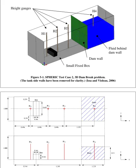
5.1 Reference Data ... 65
5.2 SPH Model of the Dam-Break Scenario ... 67
5.2.1 2D Model of the Dam-Break ... 68
5.2.2 3D Model of the Dam-Break ... 69
5.3 Summary of Free Surface Flows ... 76
6 Regular Waves in a Mesh-Free Environment ... 77
6.1 Numerically Modelling the Towing tank ... 77
6.2 Moving Floor Technique ... 81
6.3 Waves Generated using the Moving Floor Technique ... 84
6.3.1 Wave Descriptions ... 84
6.3.2 Surface Profiles ... 85
6.3.3 Through-Depth Velocity Profiles ... 87
6.3.4 Through-Depth Pressure Profiles ... 93
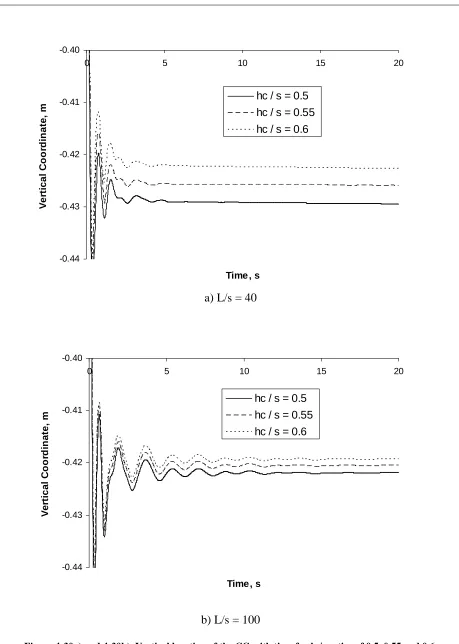
6.4 Effect of Floor Depth ... 94
6.5 Summary of Regular Waves in a Mesh-Free Environment ... 96
7 Prediction of Ship Response in Regular Waves using SPH ... 98
7.1 Reference Data ... 98
7.2 SPH Simulation Setup ... 99
7.3 Tank Width, Tank Depth and Contact Thickness Effects ... 101
7.3.1 Tank Width Effects ... 101
B K Cartwright, 2012. p.7
7.3.3 Contact Thickness Effects... 103
7.4 Pitch and Heave at Froude Numbers of 0.25 and 0.5 ... 104
7.5 Discussion of Ship Motion Predictions using SPH ... 106
8 Conclusion ... 108
9 Future Work ... 109
10 References ... 111
Appendices ... 115
A1 Abbreviations ... 115
A2 Glossary ... 116
A3 Axes Systems ... 117
A4 Bifilar Suspension ... 118
B K Cartwright, 2012. p.8
1 Introduction
1.1 Motivation
The motivation for this research was to explore the use of a generic hybridised mesh-free and finite element method as a universal tool for the prediction of the structural response of a floating structure to waves.
The vision was to have one software tool that can predict both the global motions, and the global and local structural response, including damage, of a floating, or sinking, structure subjected to any wave scenario. Such a capability was envisaged to be useful to the
assessment of not only monohull vessels, but also multihull and small water-plane area twin hull (SWATH) vessels, submarines, off-shore structures, high-speed and lightweight vessels. It could also turn out to be useful in the investigation of the response of structures which accidentally found themselves in or on the water, such as ditching of aircraft or helicopters, or the human body itself in a boat subjected to violent wave forces.
In practise, validating the vision was a bold task. Hence, the research presented here has focused on establishing the groundwork for the vision by:
a. restricting the scope to that of a rigid-ship motion response in regular waves; and b. comparing these results to tank tests and linear theory predictions.
The vision to have one software tool to conduct the complete hydrodynamic and structural response prevails. It is hoped the work here will be continued, and some recommendations to achieve this are presented in Chapter 9, Future Work.
1.2 Aim of the Current Work
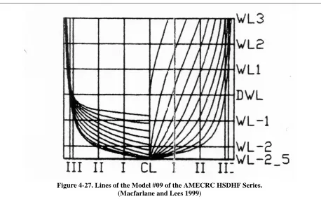
The aim of the current work was to build confidence in mesh-free methods by comparing the numerical simulation predictions to conventionally generated results from model towing tank tests and linear theory. One specific hull at two speeds in regular head waves has been compared.
The hull form used was a hull developed by the Australian Maritime Engineering
B K Cartwright, 2012. p.9
1.3 Approach to the Present Work
Mesh-free methods are emerging in various sectors of the maritime sector but are not yet commonplace. As they are not commonplace yet, a number of simple steps were taken in this research to build confidence in the mesh-free approach for ship motions. Exploring the buoyant force on some submerged shapes in two and three dimensions with this mesh-free method allowed some hydrostatic concepts to be validated. Next, the simulation of the classical dam break scenario provided some validation of the method’s ability to handle various free surface conditions such as splash and the interaction between the fluid and a rigid body.
Non-diminishing regular waves in a mesh-free fluid domain have not been demonstrated previously in the literature. A novel technique to achieve such waves in a mesh-free domain has been developed in the course of this research. The waves developed by this approach are presented for a variety of wave frequencies.
Finally the mesh-free predictions of motions for a vessel in regular waves will be presented and compared to results for the same vessel in tow tank testing and from an industry-standard linear theory panel method.
1.4 Use of a Robust Code
B K Cartwright, 2012. p.10
2 Theoretical Background
2.1 Mesh-Based Methods
The traditional numerical analysis of a fluid’s dynamical behaviour over time relies on the subdivision in space of the fluid into smaller pieces that can be analysed individually (Liu 2002). The behaviour of the system of smaller pieces taken as a whole over the time-frame in question then describes the original complete system. The process of producing these smaller pieces is called discretisation, which involves the use of cells or elements to represent either the fluid body, a Lagrangian discretisation, or the space in which the fluid resides, an
Eulerian discretisation. The resulting elements are a “mesh” that represents both the geometry of the system and the connectivity of each element therein to its neighbour(s). In a
Lagrangian system, the mesh moves with the fluid. In this approach the free surface will always be at the interface of two specific elements, one filled with water the other filled with gas. In an Eulerian system, the fluid is mapped onto the mesh, and the fluid then flows through the mesh with time and the location of the free surface will be defined by the proportion of fluid and gas in any specific element.
The governing equations for the system, based on principles such as the conservation of mass, energy and momentum, and expressed as differential and partial differential equations, are written to address the changes for any single cell or element. While these equations will be similar for both the Lagrangian and Eulerian systems, there will be differences because of the different frame of references used.
Due to the different approaches being employed, there is an inherent difference in the ability of the two systems to solve specific problems (Liu and Liu 2003). When tracking the location of a moving free-surface or the interface of two materials is the aim, the Langrangian
formulation is best as the mesh moves with the interfaces. This is reliable up to the point the movements begin to severely distort the shape of the elements, and numerical stability may become a problem due to irregular shaped elements. For the Eulerian system the mesh does not distort, but instead additional computations are required to accurately locate the free surface or interface within the mesh elements.
B K Cartwright, 2012. p.11
2.2 Mesh-Free Methods
Mesh-free methods define a system by a set of points that are able to move around the domain, instead of a mesh of elements, or cells. Associated with those points are various properties. The governing equations for the system describe how the points interact with each other, taking into consideration those properties.
As the points are discrete, with no connectivity to their neighbours, one of the advantages of mesh free methods is their ability to handle large geometric distortions of the original configuration and remain numerically stable.
A specific field of mesh-free methods is the so-called Mesh-free Particle Method, or MPM, where a finite number of points is used to track both the state of the system and the motion of the system. One of the most developed of these methods is the Smoothed Particle
Hydrodynamics (SPH) technique. This was specifically developed as a system of discrete particles to describe a continuum system (Liu and Liu 2003). Importantly, the SPH method is a Lagrangian method.
Liu (2002), Vignejvic (2004), Nguyen et al (2008) and Liu and Liu (2010) provide a summary of the many, more commonly used, mesh free methods available such as the
Element-Free Galerkin (EFG) method, the Reproducing Kernel Particle Method (RKPM), the Point Interpolation Method (PIM), the Moving Particle Semi-implicit (MPS) method, and the Finite Point Method (FPM). In this work the SPH mesh-free method has been chosen
exclusively as it the most mature of the mesh-free methods available, based on the volume of published papers.
2.3 Formulation Principles for SPH
This section outlines the fundamental mathematics of the SPH formulations and is based on the book by Liu and Liu (2003). These formulations are the same as those set out by the originators of the technique Lucy (1977), and Gingold and Monaghan (1977), and are the same as those which are employed in the commercial software code PAM-CRASH (2009) which is used for this research, henceforth referred to simply as ‘the software’.
The SPH formulations are developed in the form of integrals in Liu and Liu (2003), and then converted to a discrete particle representation relevant to numerical methods. The description here commences with the interpretation at the discrete particle level.
2.3.1 Particle Approximation
B K Cartwright, 2012. p.12
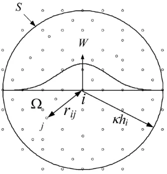
Figure 2-1 Smoothing function, W, for particle i in a 2-dimensional domain (Liu and Liu 2010).
Referring to Figure 2-1, Ω is the domain of integration and W is the smoothing function that is used to approximate field variables at some point i. The field variables of all the j particles within the cut-off distance of κ*h from i are averaged by the weight of the smoothing
function. This cut-off distance is the smoothing length h multiplied by an appropriately chosen constant κ. The extent of the domain within the cut-off distance is termed S, the support domain of W. Note that the magnitude of W depends on the distance between the points, and has h as a parameter.
The smoothing function W is chosen such that:
a) the integral over the domain is unity, the normalisation condition;
b) as the smoothing length goes to zero, not only will the value of the function approach infinity but its integral is still unity, the delta function property; and
c) the value of the smoothing function at a distance greater than the smoothing length away from the central point, is zero, the compact support condition.
In this way the field variables are represented and calculated by means of the points and the smoothing function. The material itself can also be similarly represented by assigning a volume to each point, and then using the smoothing function to find the local volume based on its neighbours by means of the smoothing function. This will now be used to summarise the characteristic equations.
The representative mass of each particle is the volume of each particle, ∆Vj, multiplied by the
density of each particle, ρj , for each of the j particles within the support domain, as follows:
mj = ∆Vj.ρj (1)
The particle approximation for the integral of the function f(x) at particle i then becomes:
= ∑ −, ℎ∆V (2)
= ∑ ౠ
ೕ
B K Cartwright, 2012. p.13 Using < > to denote a particle approximation, it is then given as:
< >= ∑ ౠ
ೕ
. (4)
And
= (−, ℎ) (5)
Equation (4) is the essence of the SPH technique as it states that the value of a function at particle i is approximated by the average of that function at all the particles within the support domain of particle i, weighted by the smoothing function.
Derivatives of the function f(x) are found by approximation also. They can be expressed as: <.>= − ∑ ౠ
ೕ
. ∇ (6)
Where
∇ = ೕ ೕ
ೕ ೕ =
ೕ ೕ
ೕ
ೕ (7)
Another key feature of the SPH technique is the implication of Equation (6), where it is stated that the derivative of a function at the particle i is approximated by the average of the values of the function at all the particles within the support domain of particle i, weighted by the gradient of the smoothing function. The important concept to note here is that it is not the derivative of the actual function which is being calculated, but instead is the derivative of the smoothing function. Hence the evaluation of the derivative of an unknown function may be simplified by using the known derivative of the smoothing kernel. Often the smoothing function is chosen such the derivative is easily calculated.
2.3.2 Support Domain and Influence Domain
The previous section used the term support domain to describe the region which is considered when determining the local value of a function.
The support domain can be centred somewhere in space that may or may not coincide with the location of one of these particles. It is important to remember that the function values at that point in space are approximated by considering the value of the function at all the particles within the support domain.
Another common term is the influence domain which is the region over which a particle exerts its influence.
In contrast to the support domain, the influence domain must be associated with a particle, and thus it represents the domain over which that particle has influence.
B K Cartwright, 2012. p.14
2.3.3 Navier-Stokes and Euler Equations
The Navier-Stokes equations are a set of partial differential equations that state the
conservation of mass, momentum and energy for a fluid. These are defined in the Lagrangian form consistent with Liu and Liu (2003) as:
Continuity:
= −
ഁ
ഁ (8)
Momentum (free of external force):
ࢻ
=
ഀഁ
ഁ (9)
Energy: = ഀഁ ഀ
ഁ (10) (The superscripts α and β are used for the coordinate directions, and summation over repeated indices is implied. ν is velocity and χ is displacement in the respective directions.)
The total stress tensor is σαβ and composed of two parts, one part the isotropic pressure p, and the other, the viscous shear stress due to dynamic viscosity, µ, as follows:
= −+ (11a)
with,
= (11b)
and, = ഁ ഀ+ ഀ ഁ− (∇. ν)δ (11c)
When the viscous component is considered negligible, the Navier-Stokes Equations without viscous term becomes the Euler Equation (Liu and Liu 2003). This affects the energy equation leaving only the pressure component as follows:
= −
ഀ
ഁ (12)
In particle approximation form, the expressions are now as follows: Continuity: = ∑ ೕ ഁ (13)
Momentum (after some manipulation, refer Liu and Liu 2003): ࢻ
= ∑
మ+
B K Cartwright, 2012. p.15 Energy: = ∑ మ+
ೕ ೕమ ೕ ഁ (15) Where
= − (16)
Liu and Liu (2003) note that the removal of the viscosity term in these equations describes an inviscid fluid, with the resulting equations then becoming simply the Euler equations. It should be noted that the software used for this research solved the Euler equations.
Liu and Liu (2010) state that many of the early algorithms did not conserve linear and angular momentum. The momentum equation stated here in equation 14, and that employed in the software used for this research, does conserve momentum as the smoothing kernel is symmetric with respect to interchange of the particle index.
2.3.4 Artificial Viscosity
Artificial viscosity is a numerical term introduced originally to control the calculation
problems associated with shock waves (Monaghan and Gingold 1983). The problem was that the shock front was typically very much smaller than the particle size, and so instabilities resulted. To overcome this, the effective width of the shock front was stretched by increasing the apparent viscosity.
For the Euler Equation where there is no real viscosity term, the velocity of the particles is modified slightly by the addition of the artificial viscosity term to the momentum equation as follows, where Π istheartificialviscosityterm:
ࢻ
= −∑
మ+
ೕ
ೕమ+ Π ೕ
ഀ
(17)
The most common form of the artificial viscosity is that proposed by Monaghan (1985), and aptly called the Monaghan artificial viscosity. The formulation is as follows:
Π = ೕ(−
ೕ
+
) (18)
Where:
(ℎ+ ℎ)
( ೕ)∙( ೕ)
ೕ
మ
"మ , (−) ∙−< 0
=
0, (−) ∙−≥ 0
B K Cartwright, 2012. p.16 In Equation (18) the α and β terms are called the alpha and beta constants of the artificial
viscosity. Monaghan, Thompson and Hourigan (1994) state that these two terms control the shear and bulk viscosity respectively, and that the shear viscosity is approximately equal to the product of α, the smoothing length and the speed of sound.
2.3.5 Equation of State
Throughout this research, one variant of the many modifications of the original Murnaghan equation of state (Murnaghan 1944) has been used. The form used states that the pressure p is given by:
= #+
బ $
− 1 (19)
Specifically, ρ/ρ0 is the ratio of the current mass density to the initial mass density, and γ is a constant equal to 7 for most applications (Monaghan, Thompson and Hourigan 1994). B is the bulk modulus of the material and is often chosen to produce a sound speed at least 10 times higher than the maximum (expected) fluid velocity. This implies that the Mach number of the flow will remain less than 0.1 which limits the density variation to about 1%, which is deemed to be a pragmatically acceptably density fluctuation that maintains the
quasi-incompressible nature of the flow regime (Monaghan, Thompson and Hourigan 1994). The Mach number also influences the time step (see Section 2.3.9) and hence the overall
computational effort required to complete a simulation of given duration, and so this determination of the minimal Mach number to retain essential flow characteristics is a convenient tool for reducing computation time.
A cut-off pressure is included in the implementation of this equation of state in the software as a simple cavitation model. In this role when the pressure of the material equals that of the cut-off pressure, the material strength is reduced to zero.
Another commonly used equation of state is the polynomial equation of state:
= #++++%+&+' (20) Where Ei is the internal energy and C0 to C6 are material constants and the terms C2µ2 and C6µ2 are set to zero if :
< 0; + 1 =/#
Toso (2009) studied the impact of deformable structures on water using SPH to represent the water, and found very similar simulation results between these two equations of state when similar properties were used in each. Toso (2090) also reported that good correlation with experimental results was maintained with a significant reduction in computation time when the speed of sound was reduced in the Murnaghan equation following the guidelines of Monaghan, Thomson and Hourigan (1994), however the correlation between experiment and prediction by SPH deteriorated when the speed of sound was reduced further.
B K Cartwright, 2012. p.17 equation of state is preferred for its ability to have a larger time-step and has thus been
chosen for this research.
2.3.6 Density Re-Initialisation
Density is commonly approximated by the particle approximation method. Density is vital for calculations in fluid dynamics, as many of the equations of state used to define a fluid contain a density term (Liu and Liu 2003).
A representation of the density in particle form is:
= ∑ (21)
This definition encounters problems when the particle is close to the domain boundary, as the cut-off distance of the smoothing function will extend beyond the domain, effectively
including a partially null volume. The consequence of this is the calculation for the density will be incorrect.
As noted in Liu and Liu (2010), a common way to overcome this resulting error is to normalise the smoothing function at the boundary by the sum of the smoothing function truncated to the domain limits. Recall from Section 2.3.1 that one of the features of the smoothing function is that the integral over its support domain is unity. Hence, if the integral is not unity, then the result is scaled accordingly. This preserves density at the boundaries. Fluctuations in density are commonly seen in various SPH formulations (Rogers et al 2009). A common technique that overcomes these fluctuations is the re-initialisation of the density field using a Shepard filter (Shepard 1968). Using this filter, which is an interpolation function, the density is periodically reinitialised as:
( = ∑ !() (22)
Where:
()
! = ೕ
∑ೕ ഐೕೕ ౠ
(23)
Equations 22 and 23 state that the individual density of some particle i is reinitialised to the total average density across the domain. Such re-initialisations done regularly during the time-frame in question leads to smoother density gradients, which in turn then leads to smoother pressure gradients throughout the domain in question. The default interval for density re-initialisation in the software used here was every 20 time-steps.
2.3.7 Anti-Crossing Parameter
B K Cartwright, 2012. p.18 displacement of particular particles such that their velocity is closer to the average within the smoothing length of that particular particle (PAM-CRASH 2009). The particles displacement is modified, conserving momentum, according to:
+
+ =+ ∑
ೕ(ೕ )
ೕ
(24)
Specifically, ε is a factor between 0 and 1, with a value of 0.5 found to work well for many scenarios (Monaghan, Thompson and Hourigan, 1994), and ρij is the density of particle j
relative to particle i.
2.3.8 Smoothing Length
The smoothing length is a dimension that, in conjunction with the parameter κ described earlier, determines the cut-off distance of the compact support of the smoothing function. The larger the smoothing length, then the larger that the influence domain of a particle will be, producing more gradual changes of parameters with distance, thus making for a more viscous-like behaviour, in the case of fluid motion.
Formulations for compressible fluids can employ a variable smoothing length that aims to maintain a constant number of neighbours within the calculation, thus ensuring effective smoothing behaviour of the material properties. For a quasi-incompressible fluid however, a constant value may be used (Monaghan, Thompson and Hourigan 1994).
2.3.9 Time step
The behaviour of the fluid over time will necessarily involve some form of time integral. The increment in time used therein between consecutive calculations is termed the time step. The original SPH formulations from 1977 of Lucy, Monaghan and Gingold did not include a discussion of time step, but this is an important, indeed a fundamental and critical, feature of any numerical solution. The rules shown here are based on the requirements for a stable implementation of any time integration within the software used for this research. The time step must be such that:
a) a shockwave moving through a material does not traverse more than one element in a time step; and
b) moving SPH particles do not pass through each other in a time step.
The first requirement is fundamental to dynamic analysis by ensuring that all transient data relevant to that shockwave is both captured and maintained in the calculation at every time-step. The second ensures that all collisions are captured by ensuring the distance traversed by any two moving particles is less than the distance between the two, such that the smoothing rules fundamental to the SPH technique can take effect.
B K Cartwright, 2012. p.19 c ="
(25)
The critical distance is the smoothing length, and hence the critical time step ∆tc is defined as:
Δ# = , (26)
A more accurate determination of the critical time step considers also the artificial viscosity parameters and particle velocities, as defined in Lombardi et al (1999) as;
Δ#-./ = min ,
.. 012ౠ 3ೕ (27)
Where:
ci = speed of sound at particle i
µij = as defined for equation (18)
The speed of particles approaching one another also has to be considered to ensure that no collisions occur within a time-step. This calculation is similar to Equation (26) in that the smoothing length is the critical distance, except the particle velocity is used in place of the speed of sound. This time step is usually orders of magnitude lower than the time step determined by shockwave rule, as the particles in fluid motion are usually travelling at much less than sonic speeds.
The software employed for this research also applies a Courant-like condition to the smallest time step to ensure convergence and avoid instabilities (PAM-CRASH 2009). This involves multiplying the smallest time-step by a factor typically less than unity.
As both the material properties, the smoothing length and the minimum distance between any two particles may change with time, the time-step will also change throughout a simulation. In the software used here, safeguards to ensure a minimum time step can be defined by the user, or similarly the simulation may cease if the time step becomes less than some
predefined value.
In summary, the time step for a group of SPH particles is determined by: - the smoothing length of the SPH particles, and
- a Courant-like factor, and
- the speed of sound in the material the SPH particle is representing, or - the maximum speed of the particles.
2.4 Rigid Bodies in SPH
B K Cartwright, 2012. p.20 For studies of fluids and rigid bodies, a rigid body being a body for analysis purposes that is considered perfectly rigid, the rigid body is typically made from SPH particles that are tied together to represent the shape of the rigid body, as in Figure 2-2 from Gonzales et al (2006). Note that in Figure 2-2 the SPH particles are sufficiently small compared to the ship so as to be not recognisable individually, but visible as a textured continuum.
Figure 2-2. Rigid bodies such as ships can be defined by a set of connected SPH particles. (Gonzales et al 2006)
For three-dimensional shapes, such as ships, their representation by discrete particles is tedious to generate, and requires quite small particles to accurately reveal the features. A much more convenient way to represent the ship is to use a series of connected panels and stringers and frames as would commonly be used for the structural analysis of that ship by the Finite Element Method (FEM). Often this type of description of the hull already exists, or is very easily exported from ship hull design software. Hence, it would be convenient to use this panel model of the hull directly in an SPH solver.
Johnson et al (2001), Ubels et al (2003), Cartwright et al (2004a and 2004b), Lobovsky and Groenboom (2009), and Vignevic and Campbell (2009a and 2009b), demonstrate software that include solvers for both SPH and finite elements within the one package. Typically, the fluid behaviour is modelled by SPH, with the structural behaviour modelled by the FEM. The software employs a time step that considers both the SPH and FEM requirements enabling a stable solution for the fluid and the structure to be solved at each time step, and enables interaction of the SPH particles with the finite elements. This is in contrast to the use of two independent stand-alone solvers, one for the fluid and one for the structure, which then require an exchange of data between the two solvers at periodic intervals to achieve full fluid-structure interaction (FSI).
Once finite elements are included in the solver, the existing library of robust finite element material models, including non-linear material definitions and material failure definitions, are able to be employed simultaneously with the SPH analysis (PAM-CRASH 2009). Combining structurally deformable materials with fluids enables complex problems such as hydro-elastic analyses to be performed within the one software package (Toso 2009, Lobovsky and
B K Cartwright, 2012. p.21
2.5 Interaction of SPH with Finite Elements
The interaction of the SPH particles and finite elements is controlled by a sliding contact interface, allowing sliding interaction, but not penetration.
Bourago and Kukudzhanov (2005) present a summary of sliding contact interface techniques. In summary, such interfaces enable elements not connected by a mesh to slide past one
another without penetration.
Many of these sliding contacts use an artificially applied penalty force to prevent elements from sliding through one another. A development of this sliding contact to cater for the discrete particles interacting with shell-type finite elements is described in Lobovsky and Groenenboom (2009), and is similar to the algorithm employed in this research (PAM-CRASH, 2009). A review of contact algorithms for use between finite elements and boundary conditions is presented in Groenenboom (2011).
The penalty force sliding contact algorithm performs a test for SPH particles that have penetrated within a predefined distance of the shell element called the “contact thickness”. Any particles that are within this contact thickness have a penalty force applied to them that is proportional (user-defined to be linear (default) or non-linear) to the depth of penetration. The force is normal to the face of the shell element face and pushes the particle away from the shell element. Particles further away than the contact thickness experience no force from the contact. As the penalty force is proportional to the penetration depth, the sliding contact acts like a spring, such that for a particle that is continually forced against the shell, say due to hydrostatic pressure on the bottom of a ship hull, equilibrium is only achieved with a small degree of penetration. Typically the penetrations for equilibrium are very small, a fraction of a percent of the contact thickness, so that the penetration is negligible on the scale of the particles and the finite element.
Sliding interfaces may also include friction laws. The software used for this research includes a variety of friction laws (PAM-CRASH, 2009), ranging from classical Coulomb friction, friction dependent on either pressure or velocity or both, friction described by standard mathematical functions, through to directionally dependent friction and even user-defined friction models. This research used effectively zero friction between the finite elements by selecting the default Coulomb friction law and then specifying a coefficient of friction of zero. This approach may need to be reconsidered if viscous effects such as drag on the body are to be considered.
2.6 Symmetry Conditions
B K Cartwright, 2012. p.22
2.7 Alternative Momentum Equations
The scenarios studied in this research considered that the presence of air on the free surface of the water is negligible. Consequently the air has not been included in the SPH simulations. For situations where the presence of air is important, such as accounting for the cushioning effects of air in a slamming event between a structure and water (Kalis 2007), the momentum equation of Equation (14) does not work well. The reason being the density of the fluids becomes smeared at density inhomogeneities, thus giving spurious results (Liu and Liu 2003). The alternative momentum equation is more suitable for these situations as follows:
ࢻ
= ∑
ೕ . ೕ
ೕ ഀ
(28)
2.8 Scaling of SPH Particles
In numerical simulations it is often necessary to use SPH particles of different size. Reasons for this could be any of the following:
a) the domain size is made larger but the number of SPH particles need to remain constant for reasons of CPU effort, or
b) a material calibration that includes the SPH parameter set was performed at one size SPH particle, but a different SPH size has to be used in an application, possibly due to a)
c) the response of a ship model in flooding requires fine SPH, yet the same ship model with forward motion in large waves will also be conducted requiring much larger particles to maintain a manageable model size (number of SPH particles). To ensure the SPH particles have similar behaviour in numerical models of different scale, the SPH parameters must be scaled according to the factors listed in Table 2-1. This table provides scaling factors according to Froude scaling.
Table 2-1 Scale factors for SPH Models.
Parameter Scale factor
Linear Geometric scale S
Bulk Modulus of Fluid S
Alpha coefficient of artificial viscosity, αΠ 1/(S1.5)
Simulation time √(S)
Timestep √(S)
Note that the α term is a factor that has no units, however it requires scaling as it is used in the artificial viscosity expression (Equation 18) that consists of other parameters of
dimension that do not scale according to Froude scaling. The scale law quoted here for α
B K Cartwright, 2012. p.23
2.9 Key SPH Parameters
For the Murnaghan equation of state (Equation 19) that has been used throughout this research, the key SPH parameters that have been used throughout this work are given in Table 2-2.
Table 2-2 Typical values of key SPH parameters.
Parameter Description Typical Value
Smoothing Kernel Type Smoothing function Cubic Spline Smoothing Length to Radius
Ratio
Defines the sphere of influence of a particle
1.6 – 2.5 with a value of 1.8 used in this research. Artificial Viscosity Terms:
Alpha Beta
Controls shear viscosity Controls bulk viscosity
0.02 for fluids Anti-Crossing Force Modifies particle velocities
and helps with stability
0.02 Bulk Modulus Influences the Mach number
and hence the time step of the simulation
Up to 2.2e9 Pa for water, but typically 2.2e6 Pa for benign waves.
Density Re-initialisation Reduces density fluctuations in the domain
Every 20 time steps (default value).
The values in Table 2-2 are based on the sensitivity studies performed in the same software (Kallis 2007), with small changes based on the author’s own experience.
As noted in Section 2.3.9, the bulk modulus of the material influences the speed of sound in the material, and consequently the time-step. For a given duration of event that is to be simulated, the number of time-steps will influence the time to complete the simulation (as does the number of particles in the calculations). Typically it is desirable to complete the calculations as quickly as possible, so having as large a time-step as possible is of interest to provide efficient solutions.
Monaghan (1994) states that if the speed of sound is 10x that of the highest anticipated speed of the particles in the model, then the behaviour of the fluid remains stable and is suitable for the simulation of the bulk flow of the fluid. Hence this rule allows a reduced Bulk modulus to be determined based on anticipated velocities, that will allow a large time-step and the rapid completion of the calculations.
2.10 Summary of Theory and Implementation
Mesh-free methods are highly customisable, such that many of the implementations discussed in the literature have been developed for particular applications within the field of fluid or solid mechanics problems.
B K Cartwright, 2012. p.24 Mesh-free techniques, including SPH as used within this work, are not as mature as the more traditional Finite Difference (FD), Finite Volume (FV) or FEM techniques for fluid and structural mechanics problems. For this reason there is still much development being reported in the literature in the use of these methods for seemingly common applications such as water flow.
The inclusion of finite elements with mesh-free solvers employing sliding algorithms is a powerful capability that conveniently allows structural components to be included in an analysis involving fluids. This has enabled complete fluid-structure interaction to be
B K Cartwright, 2012. p.25
3 Software
The software used throughout this study has been the commercial code PAM-CRASH from ESI Group, France (PAM-CRASH, 2009). The use of the software has been made available through the Australian distributor Pacific Engineering Systems International, Pty Ltd in Sydney (trading as Pacific ESI Pty Ltd.)
3.1 PAM-CRASH
PAM-CRASH is a general purpose finite element code with an explicit solver optimised for dynamic, strongly non-linear structural mechanics. PAM-CRASH contains finite element formulations for thin shells, solid elements, membranes and beams with material models with plasticity and failure for metals, plastics, rubbers, foams and composites. Robust contact algorithms are available in the code enabling the modelling of dynamic contact between various parts within a model. A Smoothed Particle Hydrodynamics (SPH) solver is
incorporated into the explicit PAM-CRASH solver, enabling both finite elements and SPH elements to be used and solved simultaneously in the same model. The solver is able to run on multiple processors to achieve reduced computation times.
The origins of the SPH solver within PAM-CRASH are in commercial work for hyper-velocity debris impact analysis on spacecraft and ballistic protection in the mid 1990s
(Groenenboom 1997) In the late 1990s the SPH material laws were extended to include fluid laws for the application of bird-strike, fuel sloshing and explosives (PAM-CRASH, 2001). Continual development of PAM-CRASH focuses on the robust implementation of advances in the field from public literature, ensuring compatibility with the existing software and material models. The direction of the software development is driven by customers who fund specific development, and topic-based research projects for which funding is received on a competitive basis.
B K Cartwright, 2012. p.26
Table 3.1 PAM-CRASH SPH Features
Material models available for SPH Murnaghan Equation of State (Equation 19) Polynomial Equation of State (Equation 20) Elasto-plastic with damage
JWL Explosive Johnson-Cook
Kernel functions W4 B-Spline
Q-Gaussian Quartic Quadratic Cubic
Quartic Spline Smoothing Lengths options Constant or variable Artificial viscosity in tension Flag to turn on or off
Symmetry planes by ghost particles Aligned to global coord axis
Momentum formalism options Options for co-existence of homogeneous or inhomogeneous material
Density re-initialisation By use of a Shepherd filter at user-defined intervals
Interaction with finite elements Both deformable and rigid shell and solid finite elements. Interaction through contact interfaces or tied interfaces.
3.2 Previous Ship-oriented Applications of PAM-CRASH
PAM-CRASH has been used commercially to study ship-ship and ship-infrastructure collisions. Much of this work has not been published due to commercial confidentiality requests, but a few reports are available such as a report on a ship colliding with a compliant wharf structure (Kisielewicz et al 1993), and predictions of damage to colliding river barges (Grabowiecki et al 2004). These studies focused mainly on non-linear finite element
behaviour in the prediction of damage and puncture of the hulls. SPH was not used in this work.
Some of the earliest papers in the public domain referencing water and waves modelled with SPH and floating structures modelled with finite elements are the works by the author of this thesis with various colleagues.
B K Cartwright, 2012. p.27 The response of a generic naval Landing Helicopter Dock (LHD) ship was predicted at one wave length and two wave heights using PAM-CRASH (Cartwright et al 2006a). Of greater interest was the prediction of the response of a landing craft within the landing dock. No correlation to model data was made, however, as the response of the landing craft within the dock is particularly difficult to model (Bass et al 2005), the ability to reveal the motion of the landing craft within the well dock from the simulation using SPH was considered a useful outcome.
PAM-CRASH was used to demonstrate the response of a single chine powerboat using SPH in calm water as it transitions from rest through to an equilibrium planing condition at high speed (Cartwright et al 2006b).
Although many of these papers by Cartwright et al did not validate the predictions, the presented numerical simulation concepts were novel at the time.
Validated results of structures in water modelled by SPH based on the concepts presented by the 2006 publications by Cartwright et al include the study of a planning vessel in water (Overpelt 2007) and the predictions of the motions of a free-fall emergency lifeboat (Kalis 2007). Both these reports concluded that correct trends were predicted by the SPH method, however the results were found to be sensitive to the numerical SPH parameters chosen, and it was commented that the role of the SPH numerical parameters was not well understood. Overpelt et al (2006) took the work of Cartwright et al (2006a) further and correlated predictions from SPH with actual test measurements. They found favourable correlation for the LHD response and the landing craft within the well dock for the sea states examined. The work of Kalis (2007) was taken further in Groenenboom (2008), to predict the
B K Cartwright, 2012. p.28
4 Hydrostatics
4.1 Introduction
The concept of hydrostatics is so fundamental to naval architecture that it may seem strange to include a section on it in this thesis.
There are two reasons this section is necessary. The first is that the SPH technique has more commonly been applied to dynamic events than static systems, due to its inherent ability to handle splash and violent free surface events. In hydrostatics the interest is in the static location of the fluid surface relative to the ship features. This is a novel application for the SPH technique, and so a brief study on static events is warranted.
The second issue is that the SPH technique describes a continuum, in this case water, by a set of nodal points that each identify the centre of a discrete volume of water. The location of the water surface is not inherently obvious. For hydrostatics there is a need to accurately locate the surface of the water both adjacent to the air and adjacent to the floating structure,
particularly for future studies that may investigate flow into and out of a damaged structure. This section establishes some rules to address these issues that are unique to the mesh-free methods.
These studies in hydrodynamics have been considered as a subset of the larger problem consisting of a tank sufficient to develop a wave train of many wavelengths for a ship to traverse. Consequently the simulations here may appear to have low numbers of large particles. The longer term aim is to use these same sized particles in the larger tank to maintain a realistic computational effort within the realms of this research. In contrast, the use of a large number of smaller particles in the hydrostatic studies may produce less errors but the findings would not be relevant to a larger tank as the number of particles required would deem the problem size impractical.
4.2 Buoyancy Force on a Submerged Body.
4.2.1 2D Studies in a 3D world
The finite element program employed for this research uses a three-dimensional coordinate system. Two-dimensional (2D) studies were conducted in a three-dimensional (3D) space by placing restraints on all entities such that they were allowed to move only in the plane of interest.
The SPH particles used in this research were represented by a single point, which is compatible with a 2D environment. This is shown in Figure 4-1 where the fluid is
B K Cartwright, 2012. p.29 The kernel is usually defined to sum over a spherical volume, centred at a specific particle
and applying weighting factors to all other particles within the smoothing length. For a 2D simulation the kernel will only find particles within a plane and so the weighting factors must be modified to ensure the sum of the kernel is still is unity. This modification to the kernel was achieved through a 'switch' in the software that selects the 2D weighting factors instead of the default 3D factors. This switch enables studies in plane strain to be undertaken. Geometric shapes such as submerged bodies or a holding tank to contain the fluid would suffice as bar elements in a 2D environment. To reliably interact with the 3D volume of the SPH particles, the 2D entities were replaced with 3D shell elements perpendicular to the plane of interest, of depth into the plane approximately equivalent to the diameter of the SPH volume. This is merely a ‘numerical etiquette’ particular to the software used to ensure that the contact algorithms work efficiently. Again referring to Figure 4-1, the solid lines
represent impassable boundaries to the SPH particles, and consequently have a dimension in the direction normal to the plane of the particles such that they are also 3D entities.
4.2.2 Submerged Objects in 2D
The first study investigated the force responses associated with a submerged square, as shown in Figure 4-1. Due to the 2D/3D nature of the code, the forces were reacted only in the plane of the square, and the 2D square was actually a thin 3D box. The thin box was rigid and held at constant depth below the surface to enable the forces acting on it to be examined to
understand how the buoyancy forces are generated using the SPH technique.
The forces acting on a stationary submerged box are the buoyancy force of the displaced fluid and the weight of the box. In the studies here the box was held at a prescribed location in space by a displacement boundary condition that perfectly reacts the weight of the box. The only remaining forces acting on the box were those due to the SPH particles.
Penetration of the box by the SPH particles was prevented by a ‘contact interface’, as
introduced in Chapter 2. The contact interface is a numerical tool that allows two materials to come into contact with each other but prevents them from passing through each other in an un-physical way. In this way the water remains on the outside of the box, and the box displaces the water. The net contact interface force is the net force acting on the box due to the SPH particles. For a stationary box in still water, the net contact force is the buoyancy force.
To conduct these tests, a rigid square box shape (in two dimensions) was located above the water, and then forcibly moved to a location where it was fully submerged. The movement of the box was controlled by a displacement boundary condition, that is, a simple function that prescribed the motion of the box with time. The box sides were oriented at 45 degrees to the horizontal, to produce a less-violent disturbance of the free-surface – i.e. if the flat face was presented to the water surface it would create a larger impact event resulting in greater splash and waves that would require more time to dissipate before reaching equilibrium conditions.
B K Cartwright, 2012. p.30 conditions of the simulation. As gravity was applied to the model and the SPH particles
settled a uniform hydrostatic pressure develops. The approach adopted here averaged the hydrostatic pressures over the total surface of the submerged box, and thus the net buoyant force was reported, as shown by the contact interface force in Figure 4-2. The unfiltered contact force is quite noisy in this example, caused by the movement of the SPH particles as they re-arrange themselves into an equilibrium position, each one bouncing off the
submerged box. A moving average of 100 samples was used to smooth the force curve to the smooth line shown.
At time zero in Figure 4-2 the box commenced the simulation above the water, and the water began to settle under gravity. The water was largely settled at time of 1 second when the box touched the water and the first contact force is registered. The reaction force of the water on the box increased to a maximum value when the box was fully submerged and moving, then settled to a near-constant value when the vertical motion ceased. The maximum reaction force was the sum of the buoyancy and all hydrodynamic forces (such as drag) acting on the box. The box was decelerated smoothly until stopped and then held at that depth for a
suitable length of time to allow the water to settle. For the 2D studies on submerged bodies a simulation time of 20 seconds was found to give a sufficiently steady buoyancy force.
B K Cartwright, 2012. p.31
Figure 4-2. Buoyancy force acting on the submerged box. Raw and Moving Average results.
In this model the submerged square was 2m x 2m. The SPH particles were on 0.2m centres. In line with the 3D representation of the 2D model, the FE model had a finite thickness into the page, so that the walls of the box were shell elements with a finite area. The thickness into the page was set to a unit thickness based on the SPH particle spacing.
The SPH parameters used to generate the figures of Figure 4-4 are listed in Table 4-1.
Table 4-1 SPH Parameters used for Buoyancy Studies with 0.2m SPH.
Parameter Value
Smoothing length/radius 1.6
Smoothing lengths : min , max 0.0001 , 0.08
Artificial viscosity terms : α , β 0.02 , 0.02
Anti-crossing force parameter 0.02
Bulk modulus 2.2e8 Pa
Shepard density re-initialisation Every 20 cycles
The properties listed in Table 4-1 with 0.2m SPH centres gave a nominal time-step of 120 microseconds. Force output were written to the output file at 100 Hz.
The final buoyant force in this example was 8454N, which is more than the theoretical value from the Archimedes principle of 7848N. The reason for this is that the hole in the water in which the box is sitting is not quite the right size – it is too large, and hence the box is
displacing more water than it should. Similarly, the water level in the tank will have risen by the volume displaced.
Figure 4-3 illustrates in detail a box submerged in SPH particles. The main dimensions are shown. The box has side length ‘L’. The SPH particles are dispersed on a nominal centre –
-30 -20 -10 0 10
0 5 10 15 20
F
o
rc
e
,
k
N
Time, s
Fy, raw
B K Cartwright, 2012. p.32 centre distance of ‘s’. The distance between the SPH particles and the surface of the
submerged box is the contact thickness and defined as ‘hc’.
Figure 4-3. Dimensions for the buoyancy tests.
Typically the contact distance, hc, will be less than or equal to the SPH spacing. As the SPH spacing varies, then so too should the contact distance. hc/s is a non-dimensional variable used here to describe contact distance effects.
Trials were conducted with different values of hc and different sized particles to find the value of the contact distance parameter that produced the buoyancy force closest to that obtained using Archimedes principle.
Figure 4-4 shows the error in buoyancy force as a function of the hc/s ratio. Three different SPH spacings were used, namely L/s of 5, 10, 20 and 100. The error was the difference between the measured buoyancy force and the actual buoyancy force, expressed as a percentage of the theoretical buoyancy force.
In Figure 4-4, the curve for the L/s value of 5 has the steepest slope, indicating that the error in the buoyancy force is sensitive to hc/s ratio. It is also not very smooth. An L/s of 5 means that there were only 5 particles along the length of the box, which was a very coarse model. The curve for the L/s value of 10 in Figure 4-4 is much less steep and has less scatter than the curve for L/s of 5. The curve for the L/s value of 100 has the least gradient and is the most linear.
From Figure 4-4 the value of hc that corresponds to the most accurate buoyancy force is when the ratio of hc /s (contact distance to particle spacing) is about 0.6 for the square shape studied here.
c Submerged Box
Domain of SPH particles
h
cB K Cartwright, 2012. p.33 To have only five SPH particles along the length of a moving body is an absurdly coarse
model, but demonstrates some interesting behaviours that will be present no matter how small the particles. The error curve for the buoyancy force is not smooth with changing contact distance, hc. Intuitively the correct value of hc is expected to be about 0.5, that is when the SPH particles are at one radius away from the surface of the submerged body, as this is their normal spacing away from adjacent SPH particles. The error curve agrees with this in principle in that the error is least around the value of 0.5 for the particle sizes studied, and significantly away from this value the error is large, i.e. at hc = 0 and hc =1. The deviation from a straight-line relationship is an interesting feature of the curve.
A likely explanation for the not-quite straight-line behaviour of the curves in Figure 4-4 is the packing of SPH particles against the surface of the body. If the SPH particles pack uniformly against the body, for example if the body length is an exact integral number of SPH particles in length, a particular value of hc will give the correct buoyant force. If the particles do not pack uniformly against the submerged body, say there is one half an SPH particle too many to fit uniformly, then the particles will not pack uniformly and the particles will not be in their most dense arrangement. Consequently a local variation of fluid density will result and a different value of hc may be needed to displace a bit more fluid to ensure the exact buoyant force.
Figure 4-4. Buoyant force error in simulation, for various SPH sizes. (Discrete values of each data set have been joined by lines for clarity.)
This can be illustrated by considering a submerged body of spherical or hexagonal shape, as shown in Figure 4-5. If the body exactly replaces one or more SPH particles, with its boundary exactly half-way between the neighbouring SPH particles, then the neighbouring particles will pack uniformly around the body, in their usual hexagonal arrangement. The value of hc /s to give the correct buoyant force will be 0.5. If the body is slightly larger, or smaller, then the neighbouring particles are not able to pack uniformly around the body,
-40% -20% 0% 20% 40% 60%
0 0.2 0.4 0.6 0.8 1
B u o y a n c y F o rc e e rr o r, %
h /s Ratio
L/s = 5
L/s = 10
L/s = 20
L/s = 100
B K Cartwright, 2012. p.34 producing a reduced local density of the fluid. The value of hc /s will need to be larger than 0.5 to achieve the correct buoyant force.
A two dimensional study of this packing example was conducted using a 19 cell hexagonal shape, as shown in Figure 4-5. In image a) the submerged shape is exactly of the area and shape that 19 equi-spaced particles would have occupied. The value of hc /s was 0.5, and the final arrangement of SPH particles around the shape is perfectly regular on a hexagonal pattern.
When the 19 cell hexagonal shape is replaced with a circle of the same area, as shown in image b) of Figure 4-5, the SPH particles cannot pack regularly against the circle, and so arrange themselves as best they can under the forces of gravity. The result is a less dense arrangement of particles. In image c) of Figure 4-5 a square of the same area was also submerged and again the SPH particles were forced to vary from their most-dense hexagonal arrangement to accommodate the submerged shape.
The buoyant force on the circle and square was larger and smaller respectively than for the hex-based shape, indicating that a different value of hc /s is required to give the correct buoyant force for each shape.
a) b) c)
Figure 4-5. Close-up views of packing irregularities around simple shapes.
(Note – image boundaries shown here are not the SPH domain boundaries – these are snapshots within the domain with a focus on the packing around the specific shapes.)
A further observation of the SPH distribution around the shapes of Figure 4-5 is that they are not symmetrical about a vertical axis through the centre of the submerged shape. This creates a net lateral force on the submerged shape. This net force is very much geometry dependent and is significant here only because of the coarse particle sized used to illustrate the nature of the packing problem. In a more research oriented simulation, the SPH particle size would be much smaller and so the corresponding lateral force due to an unequal number of fluid particles on either side of the centre line would be significantly smaller.
B K Cartwright, 2012. p.35 From these examples it is shown that the contact interface will introduce an error into the
buoyancy calculation.
4.3 Error Limits in the Buoyant Force
An estimate of the maximum error in the buoyant force as a function of the hc /s ratio can be derived from the geometry of the submerged shapes and the limits in “reasonable” contact parameters. This estimate can then be used to determine the particle size to ensure a minimum error for a specific shape.
Maintaining perspective of the application of these techniques to a ship in waves, this study in error limits is relevant in that the volume of water for numerous wavelengths will be significanly larger than the volume of water required merely to submerge a body as shown here. There will, by necessity, be a compromise in the number of particles that can
B K Cartwright, 2012. p.36
Figure 4-6. Limits of reasonable values of the contact distance.
From these limits, the maximum area is then the area of the box with the sides lengthened by s, represented by the shaded area in the left diagram of Figure 4-6. Similarly the minimum area is a box of sides of length L minus s, as shown in the right image of Figure 4-6. A comparison of the areas calculated for the two cases shown in Figure 4-6 shows that as s becomes much smaller than L, i.e. s<<L, the error in the displaced box approaches 2s/L. Using this expression, an estimate of the maximum error in buoyancy for a given L/s ratio can be determined, as shown in Table 4-2.
Table 4-2 Maximum Error Estimate for Submerged Squares.
L/s Error
5 ~ 40%
10 ~ 20%
20 ~ 10%
40 ~ 5%
100 ~ 2%
These values are in general agreement with the curves of simulation results for submerged squares shown previously in Figure 4-4. The upper right points in Figure 4-4 show an error larger than the estimated 40% error for L/s equals 5. This can be explained by s not being much smaller than L, and also by the errors due to packing of SPH particles against rigid bodies.
SPH Elements
Rigid Box
Displaced
Volume L
L+s
hc = s hc= 0
L - s
B K Cartwright, 2012. p.37 In practice it would be advisable to use L/s ratios of 40 or greater to ensure an error of less than 5%.
It can be concluded that the error will approach zero as L/s goes to infinity, if hc is proportional to s.
These error estimates are the maximum error that would result from using the worst possible value of hc, which is when hc is the same as the SPH spacing, s. Intuitively, and from Figure 4-4, the correct hc value might seem to be closer to a value of s/2. The error with a value of hc of s/2 would be less than the errors in Table 4-1.
Similar calculations can be made for other 2D and 3D shapes, with the errors as listed in Table 4-3. Table 4-3 indicates that the error is shape dependent.
For common submerged shapes of low aspect ratio, a generic rule of thumb is necessary to provide a starting point for hydrodynamic purposes. For high aspect ratio shapes, like the plate in Table 4-3, it is likely that the generic rule of thumb for low aspect ratio shapes may not be suitable, unless L/s is suitably large.
Table 4-3 Error Estimate for Submerged 2D shapes and 3D volumes.
Dimension Shape Error
2D Square, of side length L 2s/L
2D Circle, radius R s/R
3D Sphere, radius R 1.5*s/R
3D Cube, side length L 3s/L
3D Square Plate, L square, t thick s/t
The study was extended to an L/s ratio of 40 for a box in 2D and the results are shown in Figure 4-7. This simulation was setup a little different to the previous tests as much to check the robustness of the rules and also for convenience. The difference was that the SPH
particles were defined in their initial positions on an orthogonal distribution, as is
conveniently created in the pre-processor. The particles then re-arranged themselves in the first few seconds of the simulation into the more efficient hexagonal distribution with a corresponding reduction in depth.
The L/s value of 40 required a large number of SPH particles. The computational effort for the large number of SPH particles was reduced by commencing the simulation with the box in the submerged location, and allowing the water to settle around the box.
B K Cartwright, 2012. p.38
Figure 4-7. Buoyancy Force Error as a function of L/s ratio, for hc/s = 0.5.
Using initially orthogonal spacing implies that the SPH particles will rearrange themselves into a hexagonal arrangement. This rearrangement brings with it an increase of the SPH spacing dimension of about 10%. Hence the actual hc/s ratio corresponds to about 0.55 of the original orthogonal spacing distance.
The error in the measured buoyancy force was about 1% for a L/s value of 20, and reduced to 0.01% at an L/s value of 40 in this case. This error is less than the Error Estimates of Table 4-2 because the value of hc /s was closer to the correct value (even though the correct value is not known), instead of the worst case value used for calculating the values in Table 4-2.
4.4 Spheres and Cubes
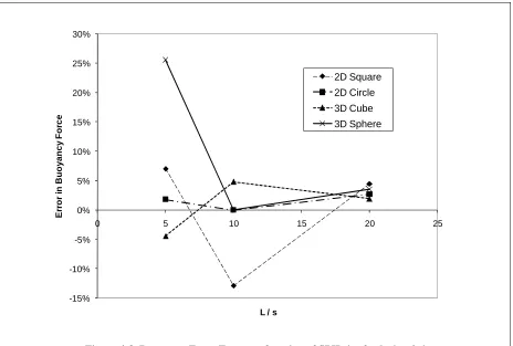
Trial simulations were also conducted in 3D to observe the trend in the measured error. The chosen volumes all had the same overall dimensions. A value of hc /s of 0.6 was chosen, based on the results for the submerged square. The error in the measured buoyancy force for different SPH particle spacing is shown in Figure 4-8.
The errors in Figure 4-8 are less than the error limits defined earlier in Table 4-3 for the 2D shapes and 3D volumes. This is to be expected as the hc /s value of 0.6 used here is lower than the maximum value of 1 used to develop the error guidelines of Table 4-3.
0% 2% 4% 6% 8% 10% 12% 14% 16%
0 10 20 30 40 50
B
u
o
y
a
n
c
y
F
o
rc
e
E
rr
o
r,
%