Contemporary geomorphological activity throughout the proglacial area of an alpine catchment

promoting access to White Rose research papers

White Rose Research Online [email protected]

Universities of Leeds, Sheffield and York

http://eprints.whiterose.ac.uk/

This is the author’s version of an article published inGeomorphology

White Rose Research Online URL for this paper:

http://eprints.whiterose.ac.uk/id/eprint/76051

Published article:

Carrivick, JL, Dickson, NE, Carver, SJ, Evans, AJ, Brown, LE, Geilhausen, M and Warburton, J (2013)Contemporary geomorphological activity throughout the proglacial area of an alpine catchment.Geomorphology, 188. 83 - 95. ISSN 0169-555X

Contemporary geomorphological activity throughout the proglacial area of

1

an alpine catchment

2 3

Jonathan L. Carrivick1*, Martin Geilhausen2, Jeff Warburton3, Neil E. Dickson1, Steve J.

4

Carver1, Andrew J. Evans1, and Lee E. Brown1

5 6

1_{School of Geography, University of Leeds, Leeds. West Yorkshire. LS2 9JT. UK} 7

2_{Department of Geography and Geology, University of Salzburg, Hellbrunnerstrasse 34, A-5020 Salzburg, Austria} 8

3

Department of Geography, Durham University, Durham, DH1 3HP, UK

9 10

*

Corresponding author:

11

Email: [email protected]

12

Tel: +44 (0) 113 34 33324

13

Fax: +44 (0) 113 34 33308

14 15 16 17

ABSTRACT 18

19

Quantification of contemporary geomorphological activity is a fundamental prerequisite for predicting 20

the effects of future earth surface process and landscape development changes. However, there is a lack 21

of high-resolution spatial and temporal data on geomorphological activity within alpine catchments, 22

which are especially sensitive to climate change, human impacts and which are amongst the most 23

dynamic landscapes on Earth. This study used data from repeated laser scanning to identify and 24

quantify the distribution of contemporary sediment sources and the intensity of geomorphological 25

activity within the lower part of a glaciated alpine catchment; Ödenwinkelkees, central Austria. 26

Spatially, geomorphological activity was discriminated by substrate class. Activity decreased in both 27

areal extent and intensity with distance from the glacier, becoming progressively more restricted to the 28

fluvially-dominated valley floor. Temporally, geomorphological activity was identified on annual, 29

seasonal, weekly and daily timescales. Activity became more extensive with increasing study duration 30

but more intense over shorter timescales, thereby demonstrating the importance of temporary storage of 31

sediment within the catchment. The mean volume of material moved within the proglacial zone was 32

4400 m3.yr-1, which suggests a net surface lowering of 34 mm.yr-1in this part of the catchment. We 33

extrapolate a minimum of 4.8 mm.yr-1net surface lowering across the whole catchment. These surface 34

lowering values are approximately twice those calculated elsewhere from contemporary measurements 35

of suspended sediment flux, and of rates calculated from the geological record, perhaps because we 36

measure total geomorphological activity within the catchment rather than overall efflux of material. 37

Repeated geomorphological surveying therefore appears to mitigate the problems of hydrological 38

studies underestimating sediment fluxes on decadal-annual time-scales. Further development of the 39

approach outlined in this study will enable the quantification of geomorphological activity, alpine 40

KEYWORDSsediment flux; landscape denudation; LIDAR-Laser scanning; glacier; river 1

2 3

HIGHLIGHTS 4

5

 Quantified distribution and intensity of contemporary geomorphological activity 6

7

 Categorisation of geomorphological activity by substrate class 8

9

 Inter-annual, seasonal, weekly and daily analysis of magnitude - frequency regime 10

11

 Mean volume of material moved within the 9.2 km2catchment of 4400 m3per year 12

13

 Net surface lowering across the whole catchment of at least 4.8 mm.yr-1 14

15 16

INTRODUCTION AND RATIONALE 17

Understanding contemporary sediment fluxes is fundamental to predicting the likely effects of future 18

changes to geomorphological activity and landscape development, whether those changes are induced 19

by climate change or by human activity (c.f. Jones, 2000; Slaymaker, 2010). Catchment-wide 20

denudation is commonly inferred indirectly from rates of fluvial suspended sediment exiting 21

catchments (c.f. Milliman and Syvitski, 1992). However, it is important to recognize that the discharge 22

of suspended sedimentfromcatchments effectively considers a catchment as a ‘black box’; it does not 23

represent all of the geomorphological activity that occurswithinthat catchment (Caine, 2004), nor does 24

it recognise the spatial and temporal variability of that activity. This problem has been acknowledged 25

for several decades by projects that have examined bedload movements and that have defined sediment 26

production, transfer and storage within a catchment (e.g. Rapp, 1960; Warburton, 1990; Trimble, 27

1995). 28

29

Future changes to geomorphological activity and landscape development will be especially rapid and 30

potentially severe within alpine catchments because they are very sensitive to climate changes and to 31

human impacts. This sensitivity is most evident in water availability (c.f. Barnett et al., 2005), water 32

quality and stream biodiversity (e.g. Brown et al., 2003; 2007), water thermal dynamics (e.g. Carrivick 33

et al., 2012) and sediment fluxes (c.f. Milliman and Syvitski, 1992; Hallet et al., 1996). Understanding 34

contemporary sediment fluxesfromalpine catchments has to account for the considerable variability in 35

geomorphological activity between adjacent mountain catchments (e.g. Gurnell et al., 1988; Trimble, 36

1995; Carrivick and Rushmer, 2009). However, understanding contemporary sediment fluxes within

37

alpine mountain catchments is complicated because mountain glacier responses to regional and local 38

a significant imbalance between sediment production and sediment transport due to former glacial 1

activity that i) over-steepens topography and promotes paraglacial slope adjustment processes, ii) 2

produces large sediment stores available for erosion, and iii) emplaces moraines that can be both a 3

sediment source and a barrier to meltwater (Beylich and Warburton, 2007). This complexity in the 4

spatial and temporal nature of geomorphological processes hinders the identification and quantification 5

of sediment sources, storages and fluxes (e.g. Dietrich and Dunne, 1978; Jones, 2000; Bertoldi, et al. 6

2009). For example, it is well known from hydrological measurements of suspended sediment that 7

small mountain catchments have a particularly variable sediment flux that is seldom resolved, partly 8

because large but short-lived events are often missed (Kirchner et al., 2001; Lewis et al., 2005). 9

Consequently, decade-long sediment-yield measurements using conventional (hydrological) methods 10

can greatly underestimate long-term (centennial – millennial) average rates of sediment delivery 11

(Kirchner et al., 2001). Short-term geomorphological activity within parts of a catchment can be 12

determined from repeated topographic measurements and episodic sediment fluxes can be calculated as 13

a volume of material moved between each of these surveys (e.g. Martin and Church, 1995; Ham and 14

Church, 2000; Fuller et al., 2003). However, whilst several European alpine countries are in the process 15

of making systematic country-wide Airborne Laser Scan surveys, use of ALS and Terrestrial Laser 16

Scan (TLS) topographic data (i.e. Light Detection and Ranging; LiDAR data) to determine 17

geomorphological changes within alpine catchments is presently limited. This is perhaps because ALS 18

datasets tend to be acquired on a campaign basis, rather than as part of routine monitoring strategies. It 19

is also undoubtedly because of the problems of processing such voluminous and complex datasets. 20

21

The overall aim of this paper is to identify and quantify the contemporary distribution and intensity of 22

activity of sediment sources, storages and fluxes within the proglacial part of a glaciated alpine 23

catchment. 24

25

QUANTIFYING GEOMORPHOLOGICAL CHANGES WITHIN ALPINE CATCHMENTS 26

Long-term (centennial-millennial) sediment storage within alpine catchments has been quantified by 27

combining geophysical surveys, digital topographic analyses and geographic information system (GIS) 28

modelling techniques (e.g. Otto et al., 2009; Schrott et al., 2003). Determination of contemporary 29

sediment sources, storages and fluxes within alpine catchments remains problematic however, not least 30

because existing catchment-wide models (e.g. Caine, 1974; Dietrich and Dunne, 1978) are qualitative. 31

These qualitative conceptual models are relied on heavily for designing contemporary field sampling of 32

definition of sediment storages and fluxes is necessary prior to a field campaign (Warburton, 1990). 1

Furthermore, it is difficult to decide how to focus field campaigns because sediment storages and fluxes 2

vary greatly over the short-term (annual-decadal) (e.g. Trimble, 1995) due to; i) functional activity of 3

geomorphological coupling is dependent on sediment availability and triggering events (Schrott et al., 4

2006), and; ii) because intermittent valley-floor and braidplain storage is very important (e.g. 5

Warburton, 1990; Orwin and Smart, 2004; Bertoldi, et al. 2009). 6

7

The best way to quantify contemporary geomorphological activity within alpine catchments; and 8

specifically to discriminate contemporary sediment storages and fluxes in space and time, is to employ 9

a geomorphological approach (i.e. to re-survey topography; e.g. Martin and Church, 1995; Ham and 10

Church, 2000; Fuller et al., 2003; Bertoldi et al., 2009). Indeed Orwin et al. (2010) recommend 11

resurveying as the most appropriate method for establishing integrated sediment flux studies in cold 12

environments on inter- and intra-annual time-scales. Re-surveying using traditional methods is 13

exceptionally time-consuming and financially expensive for anything more than a few fixed cross-14

sections of valley profiles. Differential Global Positioning Systems (dGPS) have helped to alleviate 15

these problems slightly and Schrott et al. (2006) made excellent use of photogrammetric methods to 16

determine changes in sediment storages over a four year period within a deglaciated valley in Germany. 17

Advancements in surveying technology of LiDAR; primarily in the form of ALS and TLS, for rapid 18

very high-resolution analyses (Abermann et al., 2010) have yet to be exploited for holistically 19

examining multi-scale sediment fluxes within highly dynamic alpine catchments. 20

21

LASER SCANNING OF ALPINE GEOMORPHOLOGY 22

High resolution (~ 1 m) topographic data from photogrammetry (e.g. Schrott et al., 2006) and satellite 23

image datasets from mountainous and alpine catchments have to date been used for i) 24

geomorphological mapping, ii) landform unit-scale analyses of episodic geomorphological changes, 25

and iii) analyses of river reach-scale changes (Wang et al., 2010; Smith and Pain, 2009). ALS and TLS 26

instruments give high resolution (< 1 m), high precision (> 0.2 m), and rapid acquisition of surface 27

elevation data over a range of spatial scales and are thereby revitalising geomorphological studies. 28

29

Alpine catchment-wide use of ALS and TLS datasets is still new and developing, but a notable work to 30

date is that of Van Asselen and Seijmonsbergen (2006) which illustrated that 1 m resolution Digital 31

Elevation Models (DEMs) can be analysed to map mountain hillslope and elevation properties semi-32

special attention for monitoring and measurement of retreat, downwasting, and surface character due to 1

the obvious rapid responses to, and consequences of, climate change (Abermann et al., 2010). At a 2

geomorphological unit (i.e. ‘landform’) scale (over tens of metres) and in terms of episodic event-based 3

analyses, Morche et al. (2008) used TLS data to quantify and explain changes on an alpine talus cone 4

within an alpine catchment over a four month period. Dunning et al. (2010) and Abellan et al. (2010) 5

have investigated landslide occurrence and properties. At a river reach scale, repeat surveys using 6

photogrammetric (e.g. Luchi et al., 2007), differential Global Positioning System (dGPS) (Brassington 7

et al., 2000, 2003) and remote sensing data (e.g. Lane et al., 2003) have been used to quantify changes. 8

Hetherington et al. (2005) and Milan et al. (2007) used the same data from a 10 day period in early 9

ablation season (June) to quantify a major episode of avulsion and medial bar erosion as well as 10

transient bank accretion. However, to date no studies have made repeated and multi-scale laser scan 11

surveys within an alpine catchment to identify and quantify the distribution and intensity of 12

contemporary (multi-scale) geomorphological activity and thus sediment sources, storages and fluxes, 13

holistically. 14

15

STUDY AREA DESCRIPTION 16

The Ödenwinkelkees catchment extends from ~ 47o6’00” – 47o8’7”N and from 12o37’19.5” – 17

12o40’20”E and is partially within the Hohe Tauern National Park, central Austria (Fig. 1). It is well 18

known both for its proximity to the Rudolfshutte Alpinzentrum and for the long-term measurements of 19

the snout position of the Ödenwinkelkees and of the nearby Sonnblickkees (e.g. Slupetzky, 1997; 20

Slupetzky and Aschenbrenner, 1998). The Ödenwinkelkees catchment has an area of 9.2 km2 and the 21

glacier presently occupies 1.8 km2 or 19.5 % of that area (Fig. 1A). Catchment terrain surface 22

elevations range from 1790 – 3490 m.a.s.l. (Fig. 1B). The Ödenwinkelkees catchment is composed 23

predominantly of granitic gneiss bedrock (Höck and Pestal 1994) but the hillslopes and valley floor 24

have a superficial veneer of late Holocene (Little Ice Age) and modern scree, moraine and colluvial, 25

alluvial and fluvial sediments (Slupetzky and Teufl, 1991), which are mapped in Figure 2A. The 26

Holocene (de)glacial history of the Ödenwinkelkees catchment is delimited by dated moraines, which 27

are also located inFigure 2A.Figure 3is an oblique photograph viewing south-south-eastwards from a 28

position very close to the ‘Hinterer Schafbichl’ (Fig. 1A) and it illustrates the catchment ‘mountain 29

landsystem’; specifically the geomorphological coupling between rock faces, hillslopes and moraine 30

ridges and the valley floor. The (de)glacial history (Fig. 2A) and this spatial distribution of 31

geomorphological processes (Fig. 3) led us to target three zones of interest for reporting in this paper; 32

1

DATA ACQUISITION AND PROCESSING METHODS 2

In this study we used Airborne Laser Scanner (ALS) data acquired from July 29th 2008 and multiple 3

sets of Terrestrial Laser Scanner (TLS) data acquired from July and August 2008, August 2009, and 4

June and August 2010 (Table 1). The weather conditions and river discharge during this study period 5

are depicted inFigure 4and the location of these meteorological and hydrological instruments is given 6

in Figure 1. As an overview, air temperatures were typically below zero on the Eisboden between 7

September and March, rainfall was approximately evenly distributed all summer, and river discharge 8

had a baseflow of ~ 2, a mean of 4, and peaks of 6 – 8 m3s-1 (Figure 4). More details of these 9

meteorological and hydrological data are given in Dickson et al. (2010). 10

11

AIRBORNE LASER SCANNING 12

The ALS used in this study was a Riegl Q560, which is a medium-footprint (~ 0.15 m) LiDAR system. 13

It was mounted onto the underside of a Touring Motor Glider Dimona HK36 TTC-ECO, which 14

operated at ~ 1000 m above the study area terrain. Post-processing of the ALS point cloud data was 15

performed within standard Riegl software RiAnalyse 560. Post-processing incorporated the Dimona 16

onboard dGPS data and its onboard Inertial Measurement Unit data, with dGPS base station data from 17

a Leica GPS500 dual phase receiver located at the Hinterer Schafbichl geodetic control point (Fig. 1A), 18

which is situated at 47o08 04.26241 N, 12o37’41.76277 E. This enabled georeferencing to compute the 19

3D locations of each of the ALS laser returns within the point cloud. These georeferenced points were 20

then filtered using a combination of text file editing functions to remove atmospheric clouds located 21

altitudinally above the terrain, and then standard zonal ArcGIS functions to remove atmospheric clouds 22

within valleys. The final ALS point cloud had ~ 2 returns per square metre, with elevation values for 23

each point accurate to ~ ± 0.05 m. 24

25

TERRESTRIAL LASER SCANNING 26

We used a Riegl LMS-620 and the Riegl software RiScanPro for both TLS data acquisition and data 27

processing. The maximum field of view (FOV) of this scanner is 360° horizontally and 80° vertically 28

when mounted on a tripod and levelled coarsely to 1 to 2° prior to measurement. Precise levelling was 29

performed during data processing using inclination sensor information with an accuracy of ± 0.008°. 30

To reduce the shadowing effects of large objects and a better visibility of hollows, the scanner was 31

mounted as high as possible above the surface of primary interest; i.e. usually the valley floor. At each 32

resolution scans with 0.03 - 0.04° resolution were measured leading to 41 single scans. The scanner 1

configuration was specified with 0.15 mrad beam divergence (0.045 cm footprint at 300 object 2

distance) and ‘last pulse target’ detection mode; which is useful to discriminate between ground surface 3

elements and vegetation features. TLS scan positions and reflector targets, as shown inFigure 2B, were 4

captured four to five times using the same Leica GPS system as used for ALS data acquisition, 5

resulting in an overall precision for TLS data of 2.4 ± 0.7 cm. We were unable to use reflector targets 6

for scans completed from tripod positions at higher elevation on the western valley slopes, so the 7

scanner orientation (towards North) was simply obtained with a magnetic compass (accurate to 1°). 8

This orientation was to provide a coarse georeferencing of each 3D point cloud in the early stage of 9

TLS data processing. Subsequent TLS data processing included accurate georeferencing (‘registration’) 10

and the elimination of vegetation. 11

12

Registration

13

All scan positions were levelled precisely with the inclination sensor information and georeferenced 14

using dGPS data and tie-point based (reflector) registration. The final TLS and TLS to ALS 15

registrations were achieved by means of the 'Multi Station Adjustment (MSA)', which is a semi-16

automatic least-square surface matching procedure. In general, surface matching procedures are well 17

established and have been used in different environments delivering good results (Gruen and Akca, 18

2005; Akca, 2007; Miller et al., 2008). However, TLS to ALS data registration is still a challenge and 19

Bremer and Sass (2012) recently showed that height differences of up to 0.3 m in areas without surface 20

change require further alignments. We therefore integrated the ALS data set in the MSA surface 21

matching procedure. The MSA algorithm divides the raw scan data into square tiles and reduces the 22

number of points per tile by representing them by planes based on defined criterions, e.g. maximum 23

edge length or plane error. If the deviation of the points is too high, the tile is considered not to be a 24

plane and subdivided into sub-tiles until the deviation of the points is within the criterions to define a 25

valid plane. The criteria used in this study were 5.0 m maximum edge length and 0.2 m plane error 26

deduced from several test runs to receive a high number of valid planes representing the scanned 27

surfaces. The spatial orientation and location of all scan positions was then refined in several iterations 28

to achieve the best overall fit by minimizing the normal distance between the planes of overlapping 29

scans from several scan positions and survey campaigns. Thus, all reflectors were included as reference 30

targets, all plane surfaces used were manually revised and areas of significant surface changes between 31

the surveys excluded, effects of surface discrepancies were mitigated through outlier handling and 32

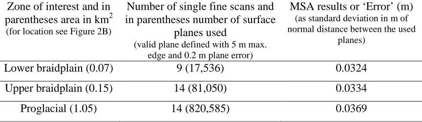
description of the MSA procedure is given in Riegl (2010). Final MSA results including the standard 1

deviation of distances between all planes used (in cm) as a measure of the final TLS and TLS to ALS 2

registration results are listed in Table 1. 3

4

Elimination of vegetation

5

The removal of vegetation is a crucial processing step as the geomorphological analyses of multi-6

temporal laser scan datasets should focus primarily on terrain changes and processes. Discrete, sparse 7

and clearly distinguishable vegetation was largely discarded during data acquisition due to the last 8

pulse detection mode. Nevertheless, sophisticated cleaning using the surface comparison functionality 9

within RiScanPro was conducted (Riegl, 2010). Therefore, point clouds were triangulated at different 10

resolutions and outliers representing vegetation were identified by comparing relatively high and low 11

resolution surfaces. However, this could not remove very dense or low vegetation, e.g. alpine meadows 12

and leafy bushes, as identified from our field notes and field photographs. In the case of small-sized 13

features points were therefore deleted manually, but in larger areas this problem remains unsolved. 14

However, the purpose of this study was to quantify geomorphological activity and it was assumed that 15

these areas were inactive due to the presence of vegetation. 16

17

DIGITAL ELEVATION MODEL (DEM) CREATION AND ANALYSIS 18

After processing, the final TLS point clouds were transferred into GIS software using the LAS file 19

format. The quality of TLS derived elevation models is influenced by i) errors caused by the laser 20

system and the applied methodology and algorithms in processing, and ii) the data and surface 21

characteristics, namely point density and type and flatness of the terrain. For this reason, rasterised 22

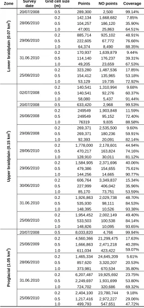
grids representing the number of points per grid cell were calculated for three point cloud resolutions; 23

0.2 m, 0.5 m and 1 m resolution and the overall coverage was calculated (Table 2). 24

25

Using a subjective consideration of the best resolution-coverage combination (Table 2), both ALS and 26

TLS point cloud data were gridded at 0.5 m cell size resolution to produce a Digital Elevation Model 27

(DEM) for each zone of interest; the ‘lower braidplain’ (0.07 km2), ‘upper braidplain’ (0.15 km2) and 28

the ‘proglacial’ zones (1.05 km2) (Fig. 2B). DEM grid cells without a point within 1 m were returned 29

with a ‘no data’ value. Each zone DEM was clipped to the extent of each substrate class that is listed 30

and mapped in Figure 2A, and as adapted from Slupetzky and Teufl (1991). For convenience and 31

brevity we use shortened versions of the substrate class names throughout the rest of this paper (e.g. 32

colluvial) and we combined the two boulder-dominated substrate classes together; ‘boulders’. We 1

differenced DEMs for the same substrate in the same zone for successive surveys and for surveys one, 2

two and three days apart, for the same substrate in the same zone at monthly intervals and the start and 3

end of each summer, and for the same substrate in the same zone at the start and end of the complete 4

study period. 5

6

The attribute table of each DEM of difference was analysed to extract the number of grid cells with a 7

given surface elevation change. To distinguish between real and artificial surface changes caused by 8

slightly varying terrain representation due to different point densities and angles of incidences, we 9

calculated DEMs of difference in defined test areas of unchanged surfaces covering approx. 100 - 200 10

m² with different surface characteristics and grain sizes. From these calculations we considered the 11

number of grid cells with surface elevation changes of > 0.15 m (Ø 0.072 ± 0.063 m) to be significant 12

for river, alluvial/colluvial and glacier terrain, and > 0.3 m (Ø 0.17 ± 0.09 m) on boulders and bedrock 13

due to the inherent roughness of these latter surfaces and the greater range of them from scan positions 14

(Fig. 2B). Thus the number of grid cells included in the DEMs of difference gives the number of 15

significant geomorphological events, the area over which these events are occurring and the total 16

volume of those events. The time period between the two surveys defining the DEM of difference 17

permitted the mean rate of volume change to be calculated. 18

19

20

SPATIAL DISTRIBUTION OF GEOMORPHOLOGICAL ACTIVITY 21

22

Our descriptions and interpretations of the elevation changes measured by the DEMs of difference are 23

informed necessarily by our knowledge of the study site. In quantification, we interpret negative 24

elevation changes as a result of erosional processes and positive elevation changes as a result of 25

depositional processes. We considered an elevation change in a grid cell to be a geomorphological 26

event and we made no attempt to link adjacent grid cells that had similar elevation changes within the 27

same time period (i.e. to identify distinct landforms). 28

29

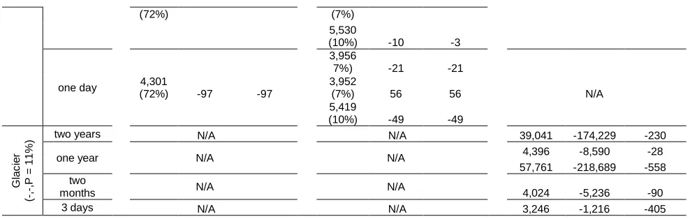
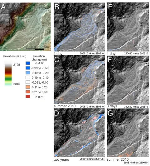
Geomorphological activity in the lower braidplain zone (Fig. 2B) was predominantly on terrain 30

produced by fluvial processes and alluvial/colluvial processes (Table 3). Fluvial processes produced 31

erosion due to gravel bank collapse (Fig. 5B), erosion due to overbank flooding and winnowing (Fig.

32

5C) and erosion due to gravel bar migration and cohesive bank erosion (Fig. 5D). Volumes of sediment 33

processes. Fluvial processes produced deposition due to overbank sedimentation (Figs. 5B, 5C, 5D) 1

and gravel bar migration (Figs. 5D, 5E), which together comprised ~ -70 m3 of sediment over three 2

days (Table 3). Irrespective of timescale of observation, it can be seen clearly from Table 3 that 3

geomorphological activity occurred across virtually the whole valley floor in the lower braidplain zone; 4

activity is not discrete. Whilst geomorphological activity that occurred in alluvial/colluvial zones was 5

widespread, the magnitude of activity was highly spatially heterogeneous; episodic erosion and 6

deposition within a gully (Figs. 5E, 5F, 5G) proceeded with volumes up to 97 m3per day (Table 3). 7

8

The upper braidplain zone (Fig. 6A) was more geomorphologically active than the lower braidplain 9

both in coverage of activity and in magnitude (Table 3). This activity was dominated both in areal 10

extent (up to 94%) and in rate of material (up to 68 m3day-1) by the active river (Table 3). Overall, this 11

geomorphological activity produced discrete erosion along sections of the braided river gravel banks 12

(Fig. 6B), erosion of a moraine ridge (Fig. 6B), erosion of hillslope (alluvial/colluvial) sediments (Fig.

13

6C) and widespread erosion of gravel bar surfaces by overbank flooding (Fig. 6D). Unlike the lower 14

braidplain, the upper braidplain appeared to be a zone of net surface lowering; i.e. erosion, with typical 15

mean rates of erosion of ~ 0.5 m3day-1 (Table 3). Deposition across the upper braidplain was 16

predominantly a result of fan apex aggradation (Figs. 6B, 6D) but some discrete positive elevation 17

changes appear to be due to gravel bar migration (Figs. 6B, 6C, 6D). Some of the speckled positive 18

elevation changes in Figures 6B and 6C were undoubtedly due to vegetation growth and were not 19

considered further. The relatively high volumes and rates for the upper braidplain boulder class (one 20

day) (Table 3) were due to melt of snowpatches and so are ignored herein. 21

22

Due to its highly variable nature, we draw attention to the fan apex at the head of the upper braidplain 23

part of the river. Within two separate three-day periods this fan experienced either intense channel 24

migration and avulsions, a complete re-organisation of the surface drainage pattern (Fig. 6E), or 25

relative inactivity (Fig. 6F). Within three separate one-day periods the river eroded moraine banks (Fig.

26

6G), produced widespread fan head aggradation (Fig. 6H) or widespread fan head lowering (Fig. 6I). 27

28

Geomorphological activity in the proglacial zone (Fig. 7A) was most widespread and most intensive 29

when compared to the other two areas of the catchment (Table 3). The glacier both retreated slightly 30

and lowered in surface elevation by up to ~ -500 m3day-1 (Table 3) and there were numerous minor 31

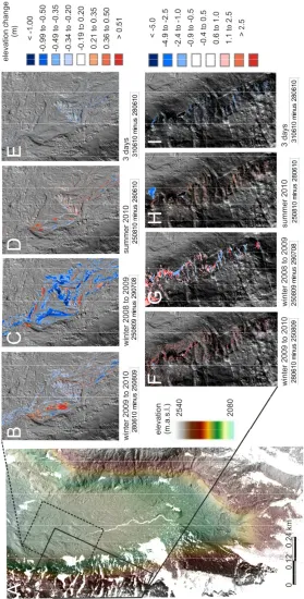
surface elevation changes on terrain categorised as alluvial/colluvial (Table 3). Figure 7 depicts a 32

and eroding gravel bars and gravel river banks (Fig. 7C). The proglacial zone of the river also had net 1

mass loss, typically of -6 m3day-1 and of up to -23 m3day-1 (Table 3). The proglacial river is clearly 2

inactive at some parts of the year; the active area in summer months (50%) and weeks (63%) is less 3

than between years (up to 91%). Terrain classified as bedrock within the proglacial zone had large areal 4

extents of activity, volumes of up to 2600 m3and rates of sediment movement of ~ 7 m3day-1 (Table 3) 5

due to episodic geomorphological activity within gullies on the flank of a prominent Little Ice Age 6

moraine ridge (Figs. 7F - 7I), and due to melt of snow patches. 7

8

Overall, 60% of the area of the Ödenwinkelkees catchment comprised landforms and land surfaces that 9

are apparently decoupled from contemporary geomorphological systems. Contemporary 10

geomorphological activity was found to be limited spatially to the Eisboden valley floor, which 11

represents 4.6 % of the catchment area, and to adjacent moraine and scree slopes covering 10.9 % of 12

the catchment area. Geomorphological activity within our study period and study area was dominated 13

by ‘continuous’ low-magnitude processes. 14

15 16

TEMPORAL INTENSITY OF GEOMORPHOLOGICAL ACTIVITY 17

Whilst we were unable to capture every geomorphological event in the Ödenwinkelkees catchment, we 18

were able to measure the aggregate effects of geomorphological activity between surveys (Table 3). 19

Thus, we can deduce the relative levels of geomorphological activity through the winter months versus 20

the summer months, for example, as we can for activity occurring within monthly, weekly and daily 21

time-scales (Table 3). Larger elevation changes are interpreted to be a result of more intense 22

geomorphological activity. 23

24

Across terrain classified as active river, the proglacial, upper braidplain and lower braidplain zones 25

experienced a mean volume change (per grid cell) over the two year study period of -5.1 m3, -0.5 m3 26

and +0.6 m3, respectively (Fig. 8). Across the winter months of 2009 – 2008 and 2009 – 2010 the 27

proglacial zone experienced a mean volume change (per grid cell) of -3.3 m3and -0.3 m3, respectively 28

(Fig. 8). In contrast, the proglacial zone had a mean volume change (per grid cell) of 1.3 m3in two 29

summer months and in the same two summer months the lower braidplain had 0.04 m3(Fig. 8). Over 30

(multiple) three day periods the active river in the proglacial, upper braidplain and lower braidplain 31

zones had mean elevation changes (per grid cell) of 2.4 m3, -0.1 m3 and 0.3 m3, and -0.3 m3, 32

m3 and 1.6 m3, and -0.4 m3, respectively. In the proglacial zone there was an order of magnitude 1

difference in this crude measure of geomorphological activity between annual and daily time periods, 2

which are characterised by net erosion and net deposition, respectively. In the upper braidplain there 3

was a trend of net erosion on annual timescales and net deposition on daily timescales, whereas in the 4

lower braidplain the reverse was observed; a trend of net deposition on annual timescales and net 5

erosion on daily timescales. 6

7

Besides the mean values described above, Figure 8 also illustrates the maximum, minimum and thus 8

the range of elevation changes for multiple time periods on terrain classified as active river. This 9

graphic (Fig. 8) thus illustrates the variability in quantified geomorphological activity on different time 10

scales. The data show that longer time periods have more variability, nor that winter months have less 11

variability than summer months, nor that the proglacial zone is more variable; i.e. has a greater range of 12

elevation changes; and thus a greater range of intensity of geomorphological activity, in any time 13

period than the upper braidplain, which is more variable than the lower braidplain (Fig. 8). 14

15

The estimated net volume change (total deposition minus total erosion) for all substrate classes 16

combined (except for the glacier and for known snow patches) over two years (Table 3) equalled 1875 17

m3 for the lower braidplain, -1313 m3for the upper braidplain, and -4035 m3for the proglacial area. 18

Across the whole area, there was a net loss of material of -5112 m3for 2009 and -3703 m3for 2010; a 19

total of -8815 m3over the two year study period. This is a mean -4407 m3 per year and hence we 20

calculated a mean surface lowering rate distributed across the combined area of the three zones of 21

interest (Fig. 2B) of -34.4 mm.yr-1. If it is assumed that the upper part of the Ödenwinkelkees 22

catchment was geomorphologically active during the study period, albeit to a lesser extent and intensity 23

than the lower part, then this volume change provides a minimum estimate of mean surface lowering 24

across the whole catchment of at least -4.8 mm.yr-1. Volumetrically, the active river accounted for -25

4118 m3(71%) out of a total of -5826 m3material moved within the lower part of the Ödenwinkelkees 26

catchment. 27

28 29

DISCUSSION: GEOMORPHOLOGICAL ACTIVITY AND DENUDATION 30

31

Sediment fluxes within alpine catchments and other cold environments are particularly affected by the 32

effects of ice and snow on the landscape (e.g. Warburton, 1999, 2007; Slaymaker, 2010) and thus are 33

glaciations, direct transport processes related to frozen water (avalanches, slush flows), ground ice 1

dynamics and phase changes of water resulting in sediment mobilisation all exert a strong control on 2

the spatial and temporal distribution and intensity of geomorphological activity and sediment fluxes 3

(Beylich and Warburton, 2007). Overall, there is some quantitative data on these discrete processes in 4

the literature but there is far less understanding of the nature of the links between them and of the 5

variability of these links (e.g. Korup, 2002). The landsystem approach does not help this understanding 6

because it cannot account for different timescales of evolution between components but also 7

importantly it cannot consider connections between different components. 8

9

Sediment fluxes from alpine and other cold environments are dominated by proglacial fluvial processes 10

(e.g. Hewitt, 2002) and research efforts into understanding sediment fluxes in alpine regions have 11

concentrated on the fluvial part of the geomorphological landsystem (e.g. Bertoldi, et al. 2009). Our 12

project is not any different in its (proglacial) focus and thus unsurprisingly our sediment flux data 13

(Table 3), which pertain to two years of representative weather conditions (Fig. 4), show a dominance 14

of the fluvial system in geomorphological activity throughout the proglacial area of the catchment. 15

However, if adjacent cells with a similar elevation change can be considered as a ‘zone’ (perhaps as a 16

landform), then adjacent ‘zones’ of erosion and deposition, and ‘zones’ that switch from erosion to 17

deposition and vice versa in our data (Figs. 5, 6 and 7, Table 3) suggest that mass movement and 18

alluvial/colluvial sources of sediment are often coupled to the fluvial system, albeit in an episodic 19

fashion. A similar finding was reported by Schrott et al. (2006) for the deglaciated Reintal Valley in 20

Germany. Consequent to such coupling, sediment transfer rates can either be extremely slow such as 21

for solifluction or very fast such as for slope failures. We also note that over very short time-scales 22

even fluvial sources of sediment in the Ödenwinkelkees catchment; i.e. glacial ice, seasonal snow and 23

groundwater/permafrost sources, were all ephemeral and thus very variable both in time and in space. 24

This variability clearly produced rapidly changing channel morphology and continual exploitation of 25

new sediment sources; Figs. 5, 6 and 7, (c.f. Warburton, 1990; Hodgkins et al., 2003; Morche et al., 26

2008). The large lateral (LIA) moraines are the dominant feature surrounding the Odenwinkelkees 27

glacier margin and these reflect glacier advance and thickening followed by stagnation and 28

downwasting; rather than glacier retreat. These moraines are clearly temporary sediment storages and 29

intermittent sediment sources (Fig. 7, Table 3). It is worthwhile noting that sediment stores within 30

alpine catchments have previously been attributed to be formed primarily by gravitational and nival 31

processes, but destroyed by fluvial processes (Schrott et al. 2006). In part, our contemporary data 32

(falls, slides, slumps) and the construction of landforms by fluvial processes (bar, bank and fan 1

aggradation). 2

3

Contemporary geomorphological activity in the Ödenwinkelkees catchment does not occur 4

homogenously in space; it is fragmented, although it does have an identifiable spatial pattern (Figs. 5, 6

5

and 7). This is perhaps not a surprise where terrain is classified as ‘active river’, but the characteristic 6

extends to other parts of the catchment that are classified as alluvial/colluvial, boulders and bedrock. 7

This ‘spatial fragmentation’ of geomorphological activity will be missed by studies solely 8

concentrating on individual landforms. Further studies should look to quantify the spatial 9

coherence/fragmentation of geomorphological activity. Furthermore, much of the geomorphological 10

activity both within the river and on hillslopes has neither a point source, nor a clearly defined transport 11

route (Figs. 5, 6 and 7). This means that studies based on within-catchment at-a-point hydrological 12

monitoring programs could be under-estimating sediment flux considerably dependent simply upon 13

study location. 14

15

For all substrate classes (except ‘glacier’) within the Ödenwinkelkees catchment we find a trend of 16

increasing area, volume and rates of sediment movement with decreasing duration between surveys 17

(Table 3). We accept that this trend could result because our shorter survey intervals were biased 18

towards the summer months, but by examining the sequential DEMs of difference (Figs. 5, 6 and 7) we 19

interpret this trend as strong indicator of the composition and behaviour of contemporary 20

geomorphological activity; specifically that erosion events are followed rapidly by depositional events 21

and vice versa. High frequency sediment transport events and geomorphological change within 22

proglacial rivers have been quantified by Ferguson et al. (1992), Ashworth et al. (1992) and Lane et al. 23

(1995), for example. Goff and Ashmore (1994) used video evidence to show that over the scale of 24

several bar lengths channel change is frequent and involves the destruction and construction of bars, 25

with sections of channel being intermittently abandoned and reoccupied. Sambrook-Smith (2000) 26

examined high-frequency proglacial sedimentation and identified preservation potential and diagnostic 27

characteristics; i.e. cyclicity with distance away from the glacier. This agrees with our results from the 28

‘lower braidplain’ zone where geomorphological events were not so intense but more frequent (Fig. 5,

29

Table 3). Similarly, but with application of repeated TLS surveys, Milan et al. (2007) reported re-30

working of proglacial river sediments by bedload transport. However, our datasets (Figs. 5, 6 and 7), 31

which are novel in being unrestricted to specific landforms and of multiple temporal intervals, 32

sediments, whether by fluvial, alluvial/colluvial or mass movement processes are common across the 1

catchment. The reworking of recently mobilised sediments, and the frequency of this geomorphological 2

activity, is herein found to be a lot more widespread and intense across alpine catchments than 3

previously measured. 4

5

Denudation rates estimated from contemporary processes need to be reconciled with those based on 6

longer-term (centennial-millennial) time-scales (Kirchner et al., 2001) Our calculated contemporary 7

mean surface lowering rate of at least 4.8 mm.yr-1 for the proglacial part of the Ödenwinkelkees 8

catchment is ~ 2.5 times that of 2 mm.yr-1 determined for; i) the last 6000 years in study of alpine 9

catchments in the Himalaya by Shroder et al. (1999), ii) late Holocene rates from British Columbia 10

(Owens and Slaymaker, 1993). It is also double the values of 0.1 – 2.6 mm.yr-1 and 0.2 – 1.4 mm.yr-1 11

most recently reported from the European Alps by Otto et al. (2009) and by Norton et al. (2011), 12

respectively. Our rate is higher than previous estimates perhaps because it pertains only to the 13

proglacial part of the catchment, perhaps because it is of unconsolidated sediment rather than bedrock, 14

and perhaps because it is a shorter (contemporary) time period of study. Additionally, and interestingly, 15

it encompasses geomorphological activity across several types of (substrate type) terrain within a 16

catchment, rather than being restricted to just sediment exiting a catchment due to fluvial processes. 17

We would suggest qualitatively that surface lowering takes place in sediments that are dominantly 18

provided by the retreating glacier. The erosion of this glacial sediment is probably decoupled from the 19

supply of this sediment. Therefore if glacial retreat rates and land surface ages could be obtained, such 20

as from dated moraines (Fig. 2A) future studies could seek to obtain a quantitative link between 21

sediment supply and land surface age; i.e. deglaciation. 22

23

There is an important need to reconcile contemporary sediment transfer rates estimated from repeated 24

geomorphological surveys with those from hydrological monitoring (Warburton, 1990). Our rate of 4.8 25

mm.yr-1for the whole Ödenwinkelkees catchment as obtained from repeated surveys is comparable to 26

the values of up to 1 - 10 mm.yr-1 presented by Hallet et al. (1996) from hydrological monitoring 27

studies and sedimentation rate measurements on mountain catchments in Alaska, British Columbia and 28

the Himalaya. It is rather less than the regional denudation rate in New Zealand calculated to be 9 29

mm.yr–1 due to a volumetric analysis of landsliding by Hovius et al. (1997), but very similar to the 30

values reported in the synthesis of contemporary mountain denudation rates by Hicks et al. (1990) from 31

sedimentation in New Zealand lakes. Whilst our rate of 4.8 mm.yr-1 includes all types of 32

deconstruct the sediment flux from an Alaskan catchment to show the effectiveness and dominance of 1

mountain glacier processes in lowering bed elevations by 1 - 2 mm.yr-1. 2

3

Hallet et al. (1996) showed a high geographical variability in denudation rates but noted a pattern of 4

increased denudation rates with total catchment area, with the volume of ice within a catchment and 5

with the discharge of water from a the catchment. However, there are a number of circumstances where 6

such relationships will not apply (Owens and Slaymaker, 1992). Hicks et al. (1990) drew attention to 7

the contrasts in glaciated versus non-glaciated catchments and Harbor and Warburton (1992, 1993) 8

advocated the relative importance of sediment storage. We also found that temporary sediment storage 9

is profoundly important. This is the reason why our mean denudation rate is relatively high; because we 10

measured total geomorphological activity, which includes intra-catchment mobilisation and temporary 11

storage, rather than a basin-averaged efflux. It is also the reason why we found that 71% by volume of 12

measured geomorphological activity within the Ödenwinkelkees catchment over a (relatively short) 13

two-year time-span was due to fluvial processes that operated across an area < 5% of the total 14

catchment. 15

16

17

CONCLUSIONS AND WIDER IMPLICATIONS 18

19

Alpine catchments are especially sensitive to climate change and to human impacts. It is imperative to 20

understand contemporary geomorphological activity within alpine catchments in order to separate these 21

impacts accurately from natural weathering rates. However, a holistic discrimination of sediment 22

sources, quantification of sediment fluxes, characterisation of geomorphological activity by substrate 23

class and the inter- and intra-annual spatial and temporal variability in these has hitherto been 24

unreported. High-resolution changes to individual landforms have been measured on an episodic 25

campaign basis, but this technique has not been applied to entire proglacial areas. Quantification of 26

geomorphological work within alpine catchments has been restricted to hydrological gauging of total 27

suspended sediment. 28

29

This study made a novel discrimination and quantification in space and time of contemporary multi-30

scale geomorphological changes within the proglacial part of a glaciated alpine catchment; the 31

Ödenwinkelkees, Austria. This permitted novel quantitative measurements of the relative importance of 32

contemporary geomorphological activity on different substrate classes to total sediment flux / 33

sediment sources; sediment input from the glacier or from rock falls in the upper catchment, such as 1

have been documented in the neighbouring Pasterze catchment (e.g. Kellerer-Pirklbauer et al., 2012) 2

were not captured due to the range of the TLS and due to the accessibility of suitable vantage points. 3

Repeated surveying permitted calculation of a net volume of material moved of 4400 m3per year in the 4

lower part of the Ödenwinkelkees catchment. This equalled 34 mm.yr-1for this part of the catchment. If 5

it is assumed that the upper part of the catchment at least has some geomorphological activity surface 6

lowering across whole catchment was at least 4.8 mm.yr-1. Repeated surveying therefore appears to 7

mitigate the problem identified by Kirchner et al. (2001) of hydrological methods underestimating 8

sediment fluxes on the annual – decadal scale. 9

10

The net volume change for all substrate classes combined (except for the glacier and for known snow 11

patches) over two years equalled 1875 m3 for the lower braidplain, -1313 m3for the upper braidplain, 12

and -4035 m3 for the proglacial area. The upper part of the proglacial area is therefore in net 13

degradation / erosion whilst the lower part is in net aggradation / deposition (Fig. 9). Geomorphological 14

activity decreased in both areal density (different substrate classes and number of pixels) and in 15

intensity (magnitude of elevation changes) from the proglacial zone to the upper braidplain zone to the 16

lower braidplain zone, i.e. with distance from glacier (Fig. 9); this is consistent with the paraglacial 17

concept. In the fluvial substrate class this relationship with distance from glacier was not smooth (Fig.

18

9) because moraines form a local topographic constriction and a locally elevated base level. Overall, 19

hillslope activity dominated in the mid-sections of the study area and fluvial activity became 20

progressively more important (areally and volumetrically) towards the lower part of the study area. The 21

summary model in Figure 9 therefore not only represents the spatio-temporal geomorphological 22

activity, but thereby infers terrain stability and the likely preservation or persistence of landforms and 23

sediments. We note that 71% of geomorphological activity by volume was restricted to < 5% of the 24

catchment area. 25

26

Temporally, there was a concentration of geomorphological activity in the Spring and Summer months, 27

which highlighted the importance of phase changes of water in alpine catchments for sediment fluxes. 28

Up to a period of two years, a longer duration of study produced more variability in active area and 29

more variability in the magnitude of elevation changes as geomorphological activity occurred 30

sporadically. Within this time period there was a dominance of continuous processes over episodic 31

processes. 32

More widely, this study provides a method by which inter-annual and inter-catchment variation (Lenzi 1

et al., 2003; Carrivick and Rushmer, 2009; Carrivick and Chase, 2011) can be quantified, and by which 2

comparison of different catchments (Gurnell et al., 1988; Beylich et al., 2006; Warburton et al., 2007; 3

Carrivick and Rushmer, 2009; Carrivick and Chase, 2011) can be made. Future studies should look to 4

i) utilise repeated ALS to determine geomorphic changes over a whole catchment, ii) quantify the 5

spatial organisation/fragmentation of geomorphological activity, and iii) quantify sediment supply with 6

land surface age; i.e. with deglaciation. With respect to these latter two topics, this study provides a 7

conceptual framework by which the contemporary importance of glacial processes versus non-glacial 8

processes can be measured (Hicks et al., 1990; Harbor and Warburton, 1992, 1993; Hallet et al., 1996), 9

and thus changes in these processes due to climate (Hodgkins et al., 2003; Stott and Mount, 2007) and 10

human impacts can be predicted. 11

12

13

ACKNOWLEDGEMENTS 14

15

ALS data was obtained by JLC and the team via a European Facility for Airborne Research (EUFAR) 16

Transnational Access award. As part of this EUFAR award Bruno Neininger piloted the aircraft and 17

Jorg Hacker provided the ALS, operated the ALS and processed the initial (raw) ALS data. Julien 18

Mocq is thanked for his ALS data processing. MG was funded by the Austrian Science Fund (FWF) 19

within the SedyMONT research project, a collaborative research project within the EUROCORES 20

programme TOPO-EUROPE of the European Science Foundation. Additional funding was provided to 21

LEB, JC and JW by a Royal Geographical Society-Institute of British Geographers with the Royal 22

Institute of Chartered Surveyors grant (GFG 39/08), and to JLC and LEB by the University of Leeds 23

Academic Development Fund for Learning and Teaching (2008). NED’s research was funded by a 24

NERC PhD studentship (NE/F008619/1). 25

REFERENCES 1

2

Abellan, A., Calvet, J., Vilaplana, J.M., Blanchard, J., 2010. Detection and spatial prediction of 3

rockfalls by means of terrestrial laser scanner monitoring. Geomorphology 119, 162-171. 4

5

Abermann, J., Fischer, A., Lambrecht, A., Geist, T., 2010. On the potential of very high-resolution 6

repeat DEMs in glacial and periglacial environments. The Cryosphere 4, 53-65. 7

8

Akca, D., 2007. Matching of 3D surfaces and their intensities. ISPRS Journal of Photogrammetry and 9

Remote Sensing 62, 112-121. 10

11

Ashworth, P.J., Ferguson, R.I., 1986. Interrelationships of channel processes, changes and sediments in 12

a proglacial braided river. Geografiska Annaler 68A, 361–371. 13

14

Ashworth, P.J., Ferguson, R.I., Ashmore, P.E., Paola, C., Powell, D.M., Prestegaard, K.L., 1992. 15

Measurements in a braided river chute and lobe; 2, Sorting of bed load during entrainment, transport 16

and deposition. Water Resources Research 28, 1887-1896. 17

18

Barnett, T.P., Adam, J.C., Lettenmaier, D.P., 2005. Potential impacts of a warming climate on water 19

availability in snow-dominated regions. Nature 438, 303-309. 20

21

Bertoldi, W., Zanoni, L., Tubino, M., 2009. Assessment of morphological changes induced by flow and 22

flood pulses in a gravel bed braided river: the Tagliamento River (Italy). Geomorphology 114, 348– 23

360. 24

25

Benn, D.I., Kirkbride, M.P., Owen, L.A. Brazier, V., 2003. Glaciated valley landsystems. In. Evans, D. 26

(Ed.), Glacial Landsystems, Hodder Arnold, London, pp. 372-406. 27

28

Beylich, A.A., Etienne, S., Etzelmüller, B., Gordeev, V.V., Käyhkö, J., Rachold, V., Russell, A.J., 29

Schmidt, K.-H., Sæmundsson, Þ., Tweed, F.S., Warburton, J., 2006. The European Science Foundation 30

(ESF) Network SEDIFLUX – An introduction and overview. In: Beylich, A.A. (Ed.), Sedimentary 31

Source-to-Sink-Fluxes in Cold Environments - SEDIFLUX. Geomorphology 80, 3-7. 32

33

Beylich, A.A., Warburton J. (Eds.), 2007. Analysis of Source-to-Sink-Fluxes and Sediment Budgets in 34

Changing High-Latitude and High-Altitude Cold Environments: SEDIFLUX Manual. First Edition. 35

NGU Report 2007.053. 158pp. 36

37

Brassington, J., Rumsby, B.T., McVey, R.A., 2000. Monitoring and modelling morphological change 38

in braided river systems using the Global Positioning System. Earth Surface Processes and Landforms 39

25, 973-990. 40

41

Brassington, J., Langham, J.A., Rumsby, B.T., 2003. Methodological sensitivity of morphometric 42

estimates of fluvial coarse sediment transport. Geomorphology 53, 299-316. 43

44

Bremer, M., Sass, O., 2012. Combining airborne and terrestrial laser scanning for quantifying erosion 45

and deposition by a debris flow event. Geomorphology 138, 49-60. 46

Brown, L.E, Hannah, D.M., Milner, A.M., 2003. Alpine stream habitat classification: An alternative 1

approach incorporating the role of dynamic water source contributions. Arctic, Antarctic and Alpine 2

Research 35, 313-322. 3

4

Brown, L.E, Hannah, D.M., Milner, A.M., 2007. Vulnerability of alpine stream biodiversity to 5

shrinking glaciers and snowpacks. Global Change Biology 13, 958-966. 6

7

Caine, N., 1974. The geomorphic processes of the alpine environment. In: Ives, J.D., Barry, R.G. 8

(Eds.), Arctic and Alpine Environments. Methuen, London, pp. 721– 748. 9

10

Caine, N., 2004. Mechanical and chemical denudation in mountain systems. In: Owens, P.N., 11

Slaymaker, O. (Eds.), Mountain Geomorphology. Arnold, London. pp. 132-152. 12

13

Carrivick, J.L., Chase, S.E., 2011. Spatial and temporal variability in the net mass balance of glaciers in 14

the Southern Alps, New Zealand. New Zealand Journal of Geography and Geophysics 54, 415-429. 15

16

Carrivick, J.L., Brown, L.E., Hannah, D., Turner, A.G.D., 2012. Numerical modelling of spatio-17

temporal thermal heterogeneity in river systems. Journal of Hydrology 414-415, 491-502. 18

19

Carrivick, J.L., Rushmer, E.L., 2009. Inter- and intra-catchment variability in proglacial 20

geomorphology: An example from Franz Josef Glacier and Fox Glacier, South Westland, New 21

Zealand. Arctic, Antarctic and Alpine Research 41, 18-36. 22

23

Dickson, N.E., Brown, L.E., Carrivick, J.L., 2010. Hydroclimatological and anthropogenic influences 24

on stream temperature dynamics of the Eisboden glacier-fed river, Austrian Alps. Proceedings of the 25

third British Hydrological Society international symposium, Newcastle, UK: pp. 726-733 26

27

Dietrich, W.E., Dunne, T., 1978. Sediment budget for a small catchment in mountainous terrain. 28

Zeitschrift für Geomorphologie. Supplementband 29, 191– 206. 29

30

Dunning, S.A., Rosser, N.J., Massey, C.I., 2010. The integration of terrestrial laser scanning and 31

numerical modelling in landslide investigations. Quarterly Journal of Engineering Geology and 32

Hydrogeology 43, 233-247. 33

34

Ferguson, R.I., Ashmore, P.E., Ashworth, P.J., Paola, C., Prestegaard, K.L., 1992. Measurements in a 35

Braided River chute and lobe: 1. Flow pattern, sediment transport, and channel change. Water 36

Resources Research 28, 1877-1886. 37

38

Fuller, I.C., Large, A.R.G., Charlton, M.E., Heritage, G.L., Milan, D.J., 2003. Reach-scale sediment 39

transfers: an evaluation of two morphological budgeting approaches. Earth Surface Processes and 40

Landforms 28, 889–903. 41

42

Goff, J.R., Ashmore, P., 1994. Gravel transport and morphological change in braided Sunwapta River, 43

Alberta, Canada. Earth Surface Processes and Landforms 19, 195–212. 44

45

Gruen, A., Akca, D., 2005. Least squares 3D surface and curve matching. ISPRS Journal of 46

Photogrammetry and Remote Sensing 59, 151–174. 47

Gurnell, A.M., Warburton, J., Clark, M.J., 1988. A comparison of the sediment transport and yield 1

characteristics of two adjacent glacier basins, Val d’Herens, Switzerland. In: Sediment Budgets 2

(Proceedings Porto Alegre Symposium December 1988) IAHS Publication 174, pp. 431–441. 3

4

Hallet, B., Hunter, L., Bogen, J., 1996. Rates of erosion and sediment evacuation by glaciers: a review 5

of field data and their implications. Global and Planetary Change 12, 213–235. 6

7

Ham, D.G. Church, M., 2000. Bed-material transport estimated from channel morphodynamics: 8

Chilliwack River, British Columbia. Earth Surface Processes and Landforms 25, 1123–1142. 9

10

Harbor, J., Warburton, J., 1992. Glaciation and denudation rates. Nature 356, 751. 11

12

Harbor, J., Warburton, J., 1993. Relative rates of glacial and non-glacial erosion processes in Alpine 13

environments. Arctic and Alpine Research 25, 1–7. 14

15

Hetherington, D., Heritage, G.L., Milan, D., 2005. Daily fine sediment dynamics on an active Alpine 16

glacier outwash plain. In: Walling, D.E., Horowitz, A.J., (Eds.), Sediment Budgets 1, IAHS Publication 17

291, pp. 278–284. 18

19

Hewitt, K., 2002. Introduction: landscape assemblages and transitions in cold regions. In: Hewitt, K., 20

Byrne, M-L., English, M., Young, G. (Eds.), Landscapes of transition: Landform assemblages and 21

transformations in cold regions. Kluwer Academic Publishers. London, pp. 1–8. 22

23

Hicks, D.M., McSaveney, M.J., Chinn, T.J.H., 1990. Sedimentation in proglacial Ivory Lake, Southern 24

Alps, New Zealand. Arctic and Alpine Research 22, 26–42. 25

26

Hodgkins, R., Cooper, R., Wadham, J., Tranter, M., 2003. Suspended sediment fluxes in a high-Arctic 27

glacierised catchment: implications for fluvial storage. Sedimentary Geology 162, 105–117. 28

29

Höck, V., Pestal, G., 1994. Geological Map of Austria 1:50.000, 153 Großglockner. Geological Survey 30

of Austria, Vienna. 31

32

Hovius, N., Stark, C.P., Allen. P.A., 1997. Sediment flux from a mountain belt derived by landslide 33

mapping. Geology 25, 231-234. 34

35

Jones, A.P., 2000. Late Quaternary sediment sources, storage and transfers within mountain basins 36

using clast lithological analysis: Pineta Basin, central Pyrenees, Spain. Geomorphology 34, 145-161. 37

38

Kirchner J.W., Finkel R.C., Clifford R.S., Granger, D.E., Clayton J.L., King J.G., Megahan, W.F., 39

2001. Mountain erosion over 10-year, 10 000-year, and 10 000 000-year timescales. Geology 29, 591– 40

594. 41

42

Kellerer-Pirklbauer, A., Lieb, G.K., Avian, M., Carrivick, J.L., 2012. Climate change and rock fall 43

events in high mountain areas: numerous and extensive rock falls in 2007 at Mittlerer Burgstall, central 44

Austria. Geografiska Annaler 94A, 59–78. 45

46

Korup, O., 2002. Recent research on landslide dams – a literature review with special attention to New 47

Zealand. Progress in Physical Geography 26, 206-235. 48

Lane, S.N., Richards, K.S., Chandler, J.H., 1995. Morphological estimation of the time-integrated 1

bedload transport rate. Water Resources Research 31, 761–772. 2

3

Lane, S.N., Westaway, R.M., Hicks, D.M., 2003. Estimation of erosion and deposition volumes in a 4

large, gravel-bed, braided river using synoptic remote sensing. Earth Surface Processes and Landforms 5

28, 249-271. 6

7

Lenzi, M.A., 2004. Displacement and transport of marked pebbles, cobbles and boulders during floods 8

in a steep mountain stream. Hydrological Processes 18, 1899–1914. 9

10

Lenzi, M.A., Mao, L., Comiti, F., 2003. Interannual variation of suspended sediment load and sediment 11

yield in an alpine catchment. Hydrological Sciences Journal 48, 899–915. 12

13

Luchi, R., Bertoldi, W., Zolezzi, G., Tubino, M., 2007. Monitoring and predicting channel change in a 14

free-evolving, small Alpine river: Ridanna Creek (North East Italy). Earth Surface Processes and 15

Landforms 32, 2104–2119. 16

17

Martin, Y., Church, M., 1995. Bed-material transport estimated from channel surveys: Vedder River, 18

British Columbia. Earth Surface Processes and Landforms 20, 347–361. 19

20

Milan, D.J., Hetherington, D., Heritage, G.L., 2007. Application of a 3D laser scanner in the 21

assessment of erosion and deposition volumes and channel change in a proglacial river. Earth Surface 22

Processes and Landforms 32, 1657–1674. 23

24

Miller, P., Mills, J., Edwards, S., Bryan, P., Marsh, S., Mitchell, H., Hobbs, P., 2008. A robust surface 25

matching technique for coastal geohazard assessment and management. ISPRS Journal of 26

Photogrammetry and Remote Sensing 63, 529-542. 27

28

Lewis, T., Braun, C., Hardy, D.R., Francus, P., Bradley, R.S., 2005. An Extreme Sediment Transfer 29

Event in a Canadian High Arctic Stream. Arctic, Antarctic, and Alpine Research 37, 477-482. 30

31

Milliman, J.D., Syvitski. J.P.M., 1992. Geomorphic/Tectonic Control of Sediment Discharge to the 32

Ocean: The Importance of Small Mountainous Rivers. The Journal of Geology 100, 525-544. 33

34

Morche, D., Schmidt, K.H., Sahling, I., Herkommer, M., Kutschera, J., 2008. Volume changes of 35

Alpine sediment stores in a state of post-event disequilibrium and the implications for downstream 36

hydrology and bed load transport. Norsk Geografisk Tidsskrift-Norwegian Journal of Geography 62, 37

89–101. 38

39

Norton, K.P., von Blanckenburg, F., DiBiase, R., Schlunegger, F., Kubik, P.W., 2011. Cosmogenic 40

10Be-derived denudation rates of the Eastern and Southern European Alps. International Journal of 41

Earth Sciences 100, 1163-1179. 42

43

Orwin, J.F., Smart, C.C., 2004. Short-term spatial and temporal patterns of suspended sediment transfer 44

in proglacial channels, Small River Glacier, Canada. Hydrological Processes 18, 1521-1542. 45

46

Orwin, J.F., Lamoureux, S.F., Warburton, J., Beylich. A., 2010. Framework for characterizing fluvial 47

sediment fluxes from source to sink in cold environments. Geografiska Annaler 92A, 155–176. 48

Otto, J-C., Schrott, L., Jaboyedoff., M., Dikau, R., 2009. Quantifying sediment storage in a high alpine 1

valley (Turtmanntal, Switzerland). Earth Surface Processes and Landforms 34, 1726–1742. 2

3

Owens, P., Slaymaker, O., 1993. Late Holocene sediment yields in small alpine and subalpine drainage 4

basins, British Columbia. In: Walling, D.E., Davies, J.R., Hasholt, B., (Eds.), Erosion, Debris flows 5

and Environment in Mountain Regions (Proceedings of the Chengdu Symposium, July 1992). IAHS 6

Publication 209, pp. 147-154. 7

8

Rapp, A., 1960. Recent developments of mountain slopes in Kärkevagge and surroundings, northern 9

Scandinavia. Geografiska Annaler 42A, 71–200. 10

11

Riegl, 2010. RiScanPro: Operating and Processing Software. Software manual. 12

13

Riihimaki, C.A., MacGregor, K.R., Anderson, R.S., Anderson, S.P., Loso, M.G., 2005. Sediment 14

evacuation and glacial erosion rates at a small alpine glacier. Journal of Geophysical Research 110, 15

F03003. 16

17

Sambrook-Smith, G.H., 2000. Small-scale cyclicity in alpine proglacial fluvial sedimentation, 18

Sedimentary Geology 132, 217-231. 19

20

Schaefer, M.R., Inkpen, 2010. Towards a protocol for laser scanning of rock surfaces. Earth Surface 21

Processes and Landforms 35, 417-423. 22

23

Schrott, L., Hufschmidt, G., Hankammer, M., Hoffmann, T., Dikau, R., 2003. Spatial distribution of 24

sediment storage types and quantification of valley fill deposits in an alpine basin, Reintal, Bavarian 25

Alps, Germany. Geomorphology 55, 45–63. 26

27

Schrott, L., Götz, J., Geilhausen, M., Morche, D., 2006. Spatial and temporal variability of sediment 28

transfer and storage in an Alpine basin (Reintal valley, Bavarian Alps, Germany). Geographica 29

Helvetica Jg. 61 2006/Heft 3 30

31

Shroder, J.F., Scheppy, R.A., Bishop, M.P., 1999. Denudation of small alpine basins, Nanga Parbat 32

Himalaya, Pakistan. Arctic, Antarctic and Alpine Research 31, 121–127. 33

34

Slaymaker, O., 2010. Drivers of mountain landscape change during the twenty-first century. Journal of 35

Soils and Sediments 10, 597-610. 36

37

Slupetzky, H., 1997. The glaciers on the topographic maps (1:5000 scale) in the region of the National 38

Park Research Station Rudolfshuette (Stubachtal, Hohe Tauern) from 1990. Wissenschaftliche 39

Mitteilungen aus dem Nationalpark Hohe Tauern [Wiss. Mitt. Nationalpark Hohe Tauern]. no. 3, pp. 40

137-162. 41

42

Slupetzky, H., Teufl, J., 1991. Ödenwinkelkees Gletschervorfeld 1:5000. Institut für kartographie und 43

reproduktionstechnik (IKR), Universität Salzburg und Oesterreichischer Alpenverein. 44

45

Slupetzky, H., Aschenbrenner, J., 1998. Stubacher Sonnblickkees, Hohe Riffel, and Alpinzentrum 46

Rudolfshütte, Austria, 1: 5,000 (Three Image Line Maps). Fluctuations of Glaciers (1990- 1995), Vol. 47

VII, World Glacier Mo-nitoring Service (WGMS) of the IUGG-FAGS/ICSI. Publ. by the ICSI of the 48

1

Smith, M.J., Pain, C.F., 2009. Applications of remote sensing in geomorphology. Progress in Physical 2

Geography 33, 568-582. 3

4

Stott, T.A, Mount, N.J., 2007. Alpine proglacial suspended sediment dynamics in warm and cool 5

ablation seasons: implications for global warming? Journal of Hydrology 332, 259-270. 6

7

Trimble, S.W., 1995. Catchment sediment budgets and change. In: Gurnell, A., Petts, G. (Eds.), 8

Changing River Channels. Wiley, Chichester, pp. 201– 215. 9

10

Van Asselen, S., Seijmonsbergen, A.C., 2006. Expert-driven semi-automated geomorphological 11

mapping for a mountainous area using a laser DTM. Geomorphology 78, 309–320. 12

13

Wang, D.M., Laffan, S.W., Liu, Y., et al. 2010. Morphometric characterisation of landform from 14

DEMs. International Journal of Geographical Information Science 24, 305-326. 15

16

Warburton, J., 1990. An Alpine proglacial fluvial sediment budget. Geografiska Annaler 72A, 261– 17

272. 18

19

Warburton, J., 1992. Observations of bed load transport and channel bed changes in a proglacial 20

mountain stream. Arctic and Alpine Research 24, 195–203. 21

22

Warburton, J., 1999. Environmental change and sediment yield from glacierized basins: the role of 23

fluvial processes and sediment storage. In: Brown, A.G., Quinne, T., (Eds.), Fluvial Processes and 24

Environmental Change. Wiley, Chichester, pp. 363–384. 25

26

Warburton, J., 2007. Sediment budgets and rates of sediment transfer across cold environments in 27

Europe: a commentary. Geografiska Annaler 89A, 95–100. 28

29

Warburton, J., Beylich, A.A., Etienne, S., Etzelmuller, B., Gordeev, V.V., Kayhko, J., Rachold, V., 30

Russell, A.J., Schmidt, H.-H., Saemundsson, P., Tweed, F.S. 2007. Editorial: Sediment budgets and 31

rates of sediment transfer across cold environments in Europe: introduction and background to the 32

European Science Foundation (ESF) Network - Sedimentary Source-to-Sink-Fluxes in Cold 33

Environments (SEDIFLUX). Geografiska Annaler 89A, 1-3. 34

Contemporary geomorphological activity throughout the proglacial area of an alpine catchment 1

2 3 4 5

Zone of interest and in parentheses area in km2

(for location see Figure 2B)

Number of single fine scans and in parentheses number of surface

planes used

(valid plane defined with 5 m max. edge and 0.2 m plane error)

MSA results or ‘Error’ (m)

(as standard deviation in m of normal distance between the used

planes)

Lower braidplain (0.07) 9 (17,536) 0.0324

Upper braidplain (0.15) 14 (81,050) 0.0334

Proglacial (1.05) 14 (820,585) 0.0369

6 7 8 9 10 11 12 13 14 15 16 17 18 19 20 21 22 23 24 25 26 27 28 29 30 31 32 33 34 35 36 37

Table 1: Number of single fine scans and plane surfaces used in the Multi Station Adjustment and 38