1
Evaluating decision making units under uncertainty using fuzzy
2multi-objective nonlinear programming
3M. Zerafat Angiz L1, M. K. M. Nawawi1 *, R. Khalid1, A. Mustafa2, A. 4
Emrouznejad3, R. John4,G. Kendall4,5
5
1School of Quantitative Sciences, Universiti Utara Malaysia, Sintok, Kedah, Malaysia. 6
2School of Mathematical Sciences, Universiti Sains Malaysia, Penang Malaysia.
7
3Aston Business School, Aston University, Birmingham, UK.
8
4ASAP Research Group, School of Computer Science, University of Nottingham, UK 9
5School of Computer Science, University of Nottingham Malaysia Campus, Malaysia 10
Abstract 11
This paper proposes a new method to evaluate Decision Making Units (DMUs) 12
under uncertainty using fuzzy Data Envelopment Analysis (DEA). In the proposed 13
multi-objective nonlinear programming methodology both the objective functions 14
and the constraints are considered fuzzy. This model is comprehensive in dealing 15
with uncertainty, in the sense that coefficients of the decision variables in the 16
objective functions and in the constraints, as well as the DMUs under assessment, 17
are assumed to be fuzzy numbers with triangular membership functions. A 18
comparison between the current fuzzy DEA models and the proposed method is 19
illustrated by a numerical example. 20
Keywords: Fuzzy DEA; membership function; fuzzy multi-objective linear 21
programming; possibility programming. 22
1. Introduction 23
Data Envelopment Analysis (DEA) is a relatively recent approach in the assessment 24
of performance of organizations and their functional units. DEA is able to evaluate 25
the Decision Making Units (DMUs) based on multiple inputs and outputs. Since the 26
first development of DEA (Banker, Charnes, & Cooper, 1984; Charnes, Cooper, & 27
Rhodes, 1978), there have been many applications of DEA in a variety of different 28
contexts (Emrouznejad & De Witte, 2010; Emrouznejad, Parker, & Tavares, 2008). 29
However in many real world applications, input or output variables are not always 30
represented by crisp values. Hence, the traditional DEA models cannot be used for 31
evaluating such DMUs. Several attempts have been made to develop fuzzy DEA 32
models that are powerful tools for comparing the performance of a set of activities or 33
organizations under uncertainty. For instance, Sengupta (1992) considered the 34
objective function to be fuzzy when utilizing a standard DEA and used 35
Zimmermann’s method (Zimmermann, 1975, 1978) to obtain the results. León et al. 36
(2003) transformed the fuzzy DEA into crisp DEA (Hougaard, 2005). Takeda and 37
Satoh (2000) used both multicriteria decision analysis and DEA with incomplete 38
data. Lertworasirikul et al., (2003a) and Lertworasirikul et al., (2003b) applied a 39
possibilistic approach (Zarafat Angiz et al., 2006) to treat the constraints of the DEA 40
as fuzzy events. Several other fuzzy models (Guo & Tanaka, 2001) have been 41
proposed to evaluate DMUs with fuzzy data, using the concept of comparison of 42
fuzzy numbers. Wen and Li (2009) proposed a hybrid method based on fuzzy 43
simulation and genetic algorithms. Recently, Emrouznejad, Tavana, and Hatami-44
Marbini (2014) provided a taxonomy and review of fuzzy DEA (FDEA) methods 45
which comprise a tolerance approach, the α-level based approach, the fuzzy ranking 46
approach, the possibility approach, the fuzzy arithmetic, and the fuzzy random/type-47
2 fuzzy set. 48
The α-cut approach (Zerafat Angiz, Emrouznejad, & Mustafa, 2012) for fuzzy DEA 49
obtained by solving another linear programming problem. The shortcoming of this 52
approach is that we lose some information about uncertainty. Further, since the 53
nature of a fuzzy linear programming (FLP) model is nonlinear, to keep all 54
information about uncertainty when solving the model, we need a nonlinear 55
programming model. In other words, in order to use a mathematical programming 56
problem to analyze the solution of an FLP problem, a multi-objective nonlinear 57
programming has the most consistency with the nature of FLP problem. 58
Alternative methodologies based on multi-objective programming are seen in 59
Zerafat Angiz, Emrouznejad, and Mustafa (2010) and Zerafat Angiz et al. (2012) 60
who introduced a new concept called local α-level which approximates the optimal 61
solution of an FLP problem by partitioning the interval of fuzzy numbers. The 62
optimal solution in this approach is based on the closeness to defuzzified points. 63
The benefit of this approach is that the multi-objective programming corresponding 64
to FLP is linear. In fact, in this approach the authors impose α-cuts together, and 65
solve a single linear programming problem. On the other hand, Zerafat Angiz et al. 66
(2010) presented a model for ranking decision making units based on a non-radial 67
approach. Saati et al. (2001) presented a non-radial model that assumed inputs and 68
outputs are fuzzy. This paper deals with a primal form of an FLP problem. Because 69
of the nature of the model, it is categorized as a pessimistic approach because the 70
worst situation of the DMU under evaluation is compared with the best situation of 71
other DMUs. 72
In this paper an optimistic approach will be presented. We propose a multi-objective 73
programming model that can retain the uncertainty in many aspects including 74
objective functions, coefficients of the decision matrix and the DMUs under 75
assessment. The discrete approach (Zerafat Angiz et al., 2012) and the proposed 76
approach follow two different views. In the discrete approach, the goal is achieving 77
benefit of applying the discrete approach is that a linear programming problem is 82
used. 83
The rest of this paper is organized as follows. A brief description of standard DEA 84
and fuzzy DEA is given in Section 2. A specific multi-objective model is discussed 85
in Section 3 and we propose an alternative fuzzy DEA model under uncertainty. 86
This is followed by a numerical illustration in Section 4. In Section 5 empirical data 87
is analyzed to illustrate the proposed approach. Section 6 presents the discussion of 88
the paper and conclusion is drawn in Section 7. 89
2. DEA and Fuzzy DEA 90
DEA is a nonparametric technique for measuring the relative efficiency of a set of 91
DMUs with multiple inputs and multiple outputs. Today, DEA has been adopted in 92
many disciplines as a powerful tool for assessing efficiency and productivity. 93
Hence, many other applications of DEA have been reported, for example hospital
94
efficiency (Tiemann, Schreyögg, & Busse, 2012), banking (Paradi & Zhu, 2013),
95
manufacturing efficiency (Jain, Triantis, & Liu, 2011), and productivity of
96
Organization for Economic Co-operation and Development (OECD) countries
97
(Emrouznejad, 2003; Lábaj, Luptáčik, & Nežinský, 2014; Prieto & Zofío, 2007).
98
Many more applications can be found in the scientific literature (Emrouznejad et al., 99
2008; Liu, Lu, Lu, & Lin, 2013) which indicates that most of these studies have 100
ignored the uncertainty in input and output values. This uncertainty could have an 101
effect on the border defined by the standard DEA; hence the CCR-DEA (Charnes et 102
al., 1978) model may not obtain the true efficiency of DMUs. Theoretically, the 103
standard CCR-DEA model has its production frontier spanned by the linear 104
combination of the observed DMUs. 105
The production frontier under uncertainty is different. The idea proposed in this 106
research is to allow some flexibility in defining the frontiers with uncertain DMUs, 107
2.1 Preliminaries
109
Definition 1 (Lai & Hwang, 1992). The α-level set (α-cut) of a fuzzy setA%is a crisp 110
subset of X and is denoted by 111
{
| A &}
Aα = x µ%≥ α x X∈ 112Definition 2. A triangular fuzzy number x% is defined as follows 113
for ( )
for l
l m
m l
x u
m u
u m
x - x
x x x
x - x µ x =
x - x
x x x
x - x
⎧
≤ ≤
⎪⎪ ⎨
⎪ ≤ ≤
⎪⎩
% (1)
m
x , xl and xu are the mean value, the lower bound and the upper bound of the 114
interval of fuzzy number (Zimmermann, 1978). The interval of fuzzy number 115
[ , ]x xl u is the region where the value of x fluctuates. Symbolically,x% is denoted by
116
(x ,x ,xm l u). Notice that there are special concepts and terminology in the Fuzzy Sets 117
Theory, when fuzzy numbers with possibilistic data are being used. In this case, xm,
118
xl and xu are called the most possible value, the most pessimistic and the most
119
optimistic values of the imprecise parameter x represented by a triangular fuzzy
120
number. For more details, see Torabi and Hassini (2008) and Pishvaee and Torabi
121
(2010).
122
2.2 Fuzzy DEA
123
The DEA technique evaluates the relative efficiency of a set of homogenous DMUs 124
by using a ratio of the weighted sum of outputs to the weighted sum of inputs. It 125
generalizes the usual efficiency measurement from a single-input, single-output ratio 126
to a multiple-input, multiple-output ratio. 127
Model 1: CCR-DEA model
131
1
1
1
max
s.t.
1
0
0
s
r rp r=
m
i ip i=
s m
r rj i ij
r= i=1
r i u y
v x =
u y - v x j
u , v r,i
≤ ∀
≥ ∀
∑
∑
∑
∑
132
where vi and ur are the weight variables for i th and r th input and output, 133
respectively. 134
At the turn of the present century, reducing complex real-world systems into precise 135
mathematical models was the main trend in science and engineering. Unfortunately, 136
real-world situations cannot usually be modelled with exact data. Thus precise 137
mathematical models are not enough to tackle all practical problems. In practice 138
there are many problems in which, all (or some) input–output levels are fuzzy 139
numbers. It is difficult to evaluate DMUs in an accurate manner to measure the 140
efficiency. Fuzzy DEA is a powerful tool for evaluating the performance of a set of 141
organizations or activities under an uncertain environment. 142
Suppose that the inputs and outputs of DMUs are fuzzy, and they are denoted by 143
( 1,2,..., )
ij
x i =% m and y r%rj ( = 1,2,..., )s respectively. Then, the CCR model with 144
fuzzy coefficients for assessing DMUpis formulated as follows: 145
1 1 1 max s.t. 1 0 0 s r rp r= m i ip i= s m
r rj i ij
r= i=1
r i
u y
v x =
u y - v x j
u , v r,i
≤ ∀ ≥ ∀
∑
∑
∑
∑
% % % % 147Saati, Memariani, and Jahanshahloo (2002) proposed a fuzzy DEA by considering 148
the α-cut of objective function and the α-cut of constraints; hence the following 149
model is obtained. 150
Model 3: Fuzzy CCR-DEA, using α-cut approach
1
1
1
1
max ( (1 ) , (1 ) )
. . ( (1 ) , (1 ) ) ( (1 ) , (1 ) )
( (1 ) , (1 ) )
( (1 ) , (1 ) ) 0
, s
m l m u
r rp rp rp rp
r m
m l m u l u
i ip ip ip ip i
i s
m l m u
r rj rj rj rj
r m
m l m u
i ij ij ij ij
i
r
u y y y y
s t v x x x x l l
u y y y y
v x x x x j
u v
α α α α
α α α α α α α α
α α α α
α α α α
= = = = + − + − + − + − = + − + − ∀ + − + − − + − + − ≤ ∀
∑
∑
∑
∑
0 , . i ≥ ∀r i 151
If we substitute ( , , )m l u ij ij ij ij
x%= x x x , y%ij =( , , )y y yijm ijl iju and1 (1,1 ,1 ) l u =
% , Model (3) is
152
written as follows. 153
Model 4: Fuzzy CCR-DEA, using α-cut approach, interval programming 155
1
1
1 1
ˆ max
ˆ . .
ˆ ˆ 0
ˆ
(1 ) (1 )
ˆ
(1 ) (1 )
(1 ) (1 )
, 0 , .
s
r rp r
m
i ip i
s m
r rj i ij
r i
m l m u
rj rj rj rj rj
m l m u
ij ij ij ij ij
l u
r i
u y
s t v x L
u y v x
y y y y y
x x x x x
l L l
u v r i
α α α α
α α α α
α α α α
=
=
= =
=
− ≤
+ − ≤ ≤ + −
+ − ≤ ≤ + −
+ − ≤ ≤ + −
≥ ∀
∑
∑
∑
∑
156
As it is shown in Saati et al. (2002) we have (1 )ll L 1
α
+ −α
≤ ≤ . One main 157drawback in Model 4 is that the optimum efficiency level occurs when the outputs of 158
the evaluated DMU and the inputs of other DMUs are set to their upper bounds, 159
while the inputs of the evaluated DMU and the outputs of other DMUs are set to 160
their lower bounds. As a result the evaluated DMU will have the largest possible 161
efficiency value; hence Model 4 may not obtain the true efficiency score. 162
In the next section we propose an alternative fuzzy DEA to tackle this problem. In 163
the suggested method the evaluated DMU will have the efficiency value between the 164
smallest and the largest possible values. 165
3. Multi-objective programming 166
Since we must solve a particular multi-objective model, a short discussion related to 167
this kind of problem is presented. 168
Consider the following multi-objective problem 169
1 2
max ( ), ( ),..., ( ) s.t. x X
n
f x f x f x
∈
In the above model, functions f x f x1( ), ( ),..., ( )2 f xn are objective functions and X is 171
considered as a feasible region. To solve the above mathematical problem, a two 172
stage procedure is proposed. 173
1. Goal of function f xi( ) i 1,2,...,n= is obtained by the following mathematical 174
programming: 175
* max ( )
s.t. x X
i i
f = f x
∈ 176
2. In this stage scale β is introduced to move functions i( )* 1 i f x
f ≤ towards their 177
optimality. For this purpose the following mathematical programming 178
problem should be solved: 179
* max
( )
s.t . i
i f x
f x X
β
β ≤
∈
180
3.1. A multi-objective fuzzy DEA model under uncertainty
181
This section proposes an alternative fuzzy DEA model. The main idea of the 182
suggested method is based on the membership functions of the coefficients. We 183
consider the coefficients as triangular fuzzy numbers(x ,x ,xm l u). Hence, the 184
membership functions of the coefficients can be defined as follows. 185
( ) ,
i j
l
i j i j l m i j i j i j m l
ij ij x i j u
i j i j m u i j i j i j m u
i j i j x x
x x x x x
x i j
x x
x x x x x
⎧ −
≤ < ⎪
− ⎪
=⎨ ∀
− ⎪
≤ ≤ ⎪ −
⎩
%
( ) ,
r j
l
r j r j l m
r j r j r j
m l
rj rj
y r j u
r j r j m u
rj r j r j
m u
r j r j
y y
y y y y y
y r j
y y
y y y y y ⎧ − ≤ < ⎪ − ⎪ =⎨ ∀ − ⎪ ≤ ≤ ⎪ − ⎩ % µ (3)
Variables xi jandyr j, in formulas (2) and (3), are representative of values in the 186
corresponding intervals of fuzzy numbers. 187
We suggest the following multi-objective nonlinear program that maximizes both 188
the objective function and the membership functions of the coefficients 189
simultaneously. 190
Model 5: A multi-objective nonlinear programming Fuzzy CCR-DEA
191
{
}
1
1
1 1
max ( ), ( )
max
. . 1
0 ( )
, ,
, 0 ,
µ µ = = = = ∀ = − ≤ ∀ ≠ ≤ ≤ ∀ ≤ ≤ ∀ ≤ ≤ ∀ ≤ ≤ ∀ ≥ ∀
∑
∑
∑
∑
%ij %rj
x ij y rj
s r rp r m i ip i s m
r rj i ij
r i
l u
ip ip ip
l u
rp rp rp
l u
ij ij ij
l u
rj rj rj
r i
x y j u y
s t v x
u y v x j j p x x x i
y y y r x x x i j y y y r j u v r i
192
Variables u vr, iindicate the coefficients of fuzzy outputs and inputs. Furthermore, 193
variables xijand yrjrepresent the intervals of fuzzy numbers x%ijandy%rj, respectively. 194
This is a multi-objective nonlinear fuzzy model that we suggest to solve in two 195
focus in this paper is to solve an FLP (Model 2) using a non-linear multi-objective 199
programming model (Model 5), not a Fuzzy multi-objective programming model 200
(FMOP). We refer readers interested in FMOP to Torabi and Hassini (2008). 201
Let us ignore the objective functions corresponding to membership functions in 202
Model 5, that is, max
{
µ
x%ij( ),xijµ
y%rj( )yrj}
. According to Zerafat Angiz et al. (2010),203
the optimal solution of the modified model will be as follows: 204
* *
* *
= ≠ =
= ≠ =
u l
ij ij ip ip
l u
rj rj rp rp
x x j p x x y y j p y y 205
This is because each DMU with inputs greater than and outputs less than inputs and 206
outputs DMUp respectively, will not be better thanDMUp. So the optimal value of 207
Model (5) is equals to efficiency ofDMUp. 208
Ignoring the last objective function in Model (5), the optimal solution will be as 209
follows: 210
* *
* *
= ≠ =
= ≠ =
m m
ij ij ip ip
m m
rj rj rp rp
x x j p x x y y j p y y 211
Interaction between two opposed objective functions specify the optimal solution. 212
Lemma1: Let’s consider the optimistic point of view that is the best condition for 213
DMU under evaluation and the worst condition for other DMUs. 214
a. The optimal solution for
µ
x%ij( ),xijµ
y%rp(yrp)are obtained in the second 215condition of the membership functions (2) and (3), respectively. 216
b. The optimal solution for
µ
x%ip( ),xipµ
y%rjʹ ( )(yrj j p≠ ) are obtained in the first 217Proof: Suppose that objective function in Model (5) be only ( 1 max =
∑
s r rp ru y ), as 219
mentioned above, due the nature of the model the optimal solution will be: 220
min max , ( )
max min , ( )
ip ij
rp rj
x i x i j j p
y r y r j j p
∀ ∀ ≠
∀ ∀ ≠ (4)
221
When considering the effect of the membership function, the values of 222
, ( )
∀ ≠
ij
x i j j p and yrp ∀r will be decreased and the values of xip ∀i and
223
, ( )
∀ ≠
rj
y r j j p will be increased (membership numbers will be zero for the above 224
mentioned values). So, to obtain the optimal solution of
µ
x%ij( ),xijµ
y%rp(yrp) the second 225condition of the membership functions (2) and (3) are sufficient, respectively. 226
Similarly to obtain the optimal value for
µ
x%ip( ),xipµ
y%ʹrj( )(yrj j p≠ ) the first condition 227of the membership functions (2) and (3) are sufficient, respectively, i.e. 228
)
5 (
( ) [ , ]
µ = − ∈ ∀
− %ip
l
ip ip l m
x ip m l ip ip ip ip ip
x x
x x x x i
x x
)
6
(
( ) [ , ]
µ = − ∈ ∀
− %rp
u
rp rp m u
y rp u m rp rp rp
rp rp
y y
y y y y r
y y
) 7
(
( ) [ , ] , ( )
µ = − ∈ ∀ ≠
−
%ij
u
ij ij m u
x ij u m ij ij ij
ij ij
x x
x x x x i j j p
x x
)
8
(
( ) [ , ] , ( )
µ = − ∈ ∀ ≠
− %rj
l
rj rj l m
y rj m l rj rj rj rj rj
y y
y y y y r j j p
y y
Let *, *( ) ≠
ij rj
x y j p and *, * ip rp
x y be the optimal solution forx y jij, rj( ≠ p)and x yip, rp. It 229
is clear that there exist two values in the intervals [ , ],[ , ] (x xijl iju y yrjl rju j p≠ )and
* *
1∈[ , ], 1∈[ , ]
l m l m
ij ij ij rj rj rj
x x x y y y
* *
2∈[ , ], 2∈[ , ]
m u m u ij ij ij rj rj rj
x x x y y y
* *
1∈[ , ], 1∈[ , ]
l m l m
ip ip ip rp rp rp
x x x y y y
* *
2∈[ , ], 2∈[ , ]
m u m u
ip ip ip rp rp rp
x x x y y y .
(9)
In this view, the x sij are similar to the input values and the y srj are similar to the 232
output values in the DEA models, so by considering constant values for x sandij y srj , 233
Model (5) will be converted to Model (4). According to Lemma 1, the best situation 234
of the DMU under evaluation is compared with the worst situation of other DMUs, 235
and this means that the evaluation is based on an optimistic approach. In Zerafat 236
Angiz et al. (2010), it is proved that the worst situation of the DMU under evaluation 237
is compared with the best situation of other DMUs, that is, a pessimistic view. A 238
discrete approach is based on defuzzified points, and two other methodologies 239
consider the mean value (most possible point) as their goals. 240
The discrete approach (Zerafat Angiz et al., 2012) and the proposed approach follow 241
two different views. In the discrete approach, the goal is achieving defuzzified 242
points whereas the goal of fuzzy numbers in the proposed approach is the most 243
possible values. The discrete approach tries to keep information about uncertainty as 244
much as possible as the new approach does. The discrete approach approximates the 245
solution, but it still loses some information about uncertainty. The benefit of 246
applying a discrete approach is that a linear programming model is used. 247
Assume that inputs and outputs ofDMUAand DMUB are * * * * 1 1 2 2
(xʹip,x yijʹ , ʹrp ,yrjʹ )(j≠ p) 248
and * * * *
2 2 1 1
(x xipʹ ijʹ ,yrpʹ ,yrjʹ )(j≠ p), respectively. ObviouslyDMUAis more efficient than
249
B
membership function (2) and (3) are sufficient to obtain the optimum value for 253
( ), ( )( )
ip ij
x xip y yij j p
µ
%ʹ ʹµ
%ʹ ʹ ≠ .254
Hence, to solve Model (5), the methodology presented in section 3 is applied, and 255
multi-objective programming problem (5) is converted to the following nonlinear 256
programming problem: 257
258
Model 6: A new Fuzzy CCR-DEA, non-linear programming
259 1 * 1 1 1 max . . 1 ( ) /
0 ( )
, ( )
, ( )
, ( ) 6.1
m
i ip i
s
r rp p
r
s m
r rj i ij
r i
u i j i j
u m
i j i j l r j r j
m l
r j rj l i p i p
m l
i p i p u
r p r p
u m
r p rp
m u
i j i j i j l
r j r
Z h
s t
v x
h u y z
u y v x j j p
x x
h i j j p
x x
y y
h r j j p
y y x x h i x x y y h r y y
x x x i j j p
y y = = = = = = ≤ − ≤ ∀ ≠ − ≤ ∀ ≠ − − ≤ ∀ ≠ − − ≤ ∀ − − ≤ ∀ − ≤ ≤ ∀ ≠ ≤
∑
∑
∑
∑
, ( ) 6.2
6.3 6.4
, 0 ,
m j rj
l m
i p i p i p
m u
r p r p rp
r i
y r j j p
x x x i
y y y r
u v r i
≤ ∀ ≠
≤ ≤ ∀
≤ ≤ ∀
≥ ∀
In Model (6), *
p
z is obtained with the best situation (optimistic view point) of the
262
DMUs as follows:
263
Model 7: A new Fuzzy CCR-DEA, estimation of Z*p 264 1 1 1 1 max . 1
0 ( )
, 0 ,
s u
p r rp
r m l i ip i s m l l
r rj i ip
r i
r i
z u y
s t v x
u y v x j j p
u v r i
= = = = = = − ≤ ∀ ≠ ≥ ∀
∑
∑
∑
∑
265Obviously, fluctuating between 0 and 1, the objective functions corresponding to 266
membership functions do not need to follow the first stage of Section 3. Z*P 267
indicates the best situation of the DMU under evaluation comparing to other DMUs. 268
Notice that Model 7 finds the optimal solution ignoring the membership values. This 269
is why we consider the largest value of outputs and smallest values of inputs 270
corresponding to the DMU under evaluation, and the smallest outputs and largest 271
inputs for the other DMUs. Therefore, in Model 6, * 1
0 ( s r rp) / p 1
r
u y z
=
≤
∑
≤ , and the272
goal will be maximum value that is 1. 273
The variable h in Model (6) is used to convert the multi-objective problem Model (5) 274
to a nonlinear programming problem. This variable is within the interval [0,1]. 275
Adding the concept of α-cut to Model (6), it is sufficient to replace the following 276
constraints instead of 6-1, 6-2, 6-3 and 6-4. 277
(1 ) , ( )
(1 ) , ( )
(1 )
m m u
i j i j i j i j
m l m
r j r j r j rj
m l m
i p i p i p i p
x x x x i j j p
y y y y r j j p
x x x x i
α α
α α
α α
ʹ ≤ ʹ ≤ ʹ + − ʹ ∀ ≠
ʹ + − ʹ ≤ ʹ ≤ ʹ ∀ ≠
This is different from the standard α-cut used in the fuzzy DEA Model (4), because 279
in each α-level the model still retains uncertainty information interior of the interval 280
that was generated by α. Next section compares our results with the current fuzzy 281
DEA model. 282
4. An illustration with a numerical example 283
In this section, a numerical example is presented to illustrate the difference between 284
the results obtained using the proposed approach and the current fuzzy DEA models. 285
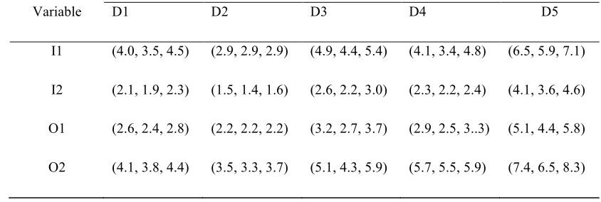
Consider the data in Table 1 that is extracted from Guo and Tanaka (2001) and used 286
by Lertworasirikul et al. ( 2003a) and Saati et al. (2002). There are 5 DMUs with 287
two symmetrical triangular fuzzy inputs and 2 symmetrical triangular fuzzy outputs. 288
Table 1: Data for numerical example
290
DMU
Variable D1 D2 D3 D4 D5
I1 (4.0, 3.5, 4.5) (2.9, 2.9, 2.9) (4.9, 4.4, 5.4) (4.1, 3.4, 4.8) (6.5, 5.9, 7.1)
I2 (2.1, 1.9, 2.3) (1.5, 1.4, 1.6) (2.6, 2.2, 3.0) (2.3, 2.2, 2.4) (4.1, 3.6, 4.6)
O1 (2.6, 2.4, 2.8) (2.2, 2.2, 2.2) (3.2, 2.7, 3.7) (2.9, 2.5, 3..3) (5.1, 4.4, 5.8)
O2 (4.1, 3.8, 4.4) (3.5, 3.3, 3.7) (5.1, 4.3, 5.9) (5.7, 5.5, 5.9) (7.4, 6.5, 8.3)
291
Using fuzzy CCR Model (4), the efficiency scores are summarized in the Table 2. 292
Table 2: The efficiencies using Model (4) 293
DMU
Α D1 D2 D3 D4 D5
0 1.107 1.506 1.276 1.525 1.296
.5 0.995 1.321 1.035 1.319 1.159
.75 0.906 1.237 0.936 1.230 1.086
1 0.852 1.000 0.863 1.000 1.000
294
Considering the above Lemma 1, the optimal solution given in Table 2 is equivalent 295
to the optimal solution related to the optimistic part of Kao and Liu (2000) approach 296
in its supper efficiency form. The methods based on the α-cut approach just extend 297
number of membership values considered in the evaluation. Therefore the major part 298
Results from the possibility approach of Lertworasirikul et al. (2003a) are shown in 303
Table 3. As can be seen, the efficiency values in the above two models are very 304
[image:18.612.101.531.197.341.2]similar. 305
Table 3: The efficiencies using Lertworasirikul et al. (2003a) model 306
DMU
α D1 D2 D3 D4 D5
0 1.107 1.238 1.276 1.520 1.3296
.5 0.963 1.112 1.035 1.258 1.159
.75 0.904 1.055 0.932 1.131 1.095
1 0.855 1.000 0.861 1.000 1.000
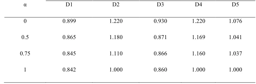
[image:18.612.101.529.428.569.2]Using the proposed Model (6), the results are shown in Table 4. 307
Table 4: The efficiencies using the proposed model in this paper 308
DMU
α D1 D2 D3 D4 D5
0 0.899 1.220 0.930 1.220 1.076
0.5 0.865 1.180 0.871 1.169 1.041
0.75 0.845 1.110 0.866 1.160 1.037
1 0.842 1.000 0.860 1.000 1.000
309
Due to the nature of the fuzzy CCR Model (4) the maximum efficiency occurs when 310
the outputs of the evaluated DMU and the inputs of other DMUs are set to their 311
upper bounds. It is obvious that the results in Table 2 are always greater than the 312
this paper have the efficiency values between the smallest and the largest possible 315
values, hence they are more close to the true efficiency. 316
5. Empirical study 317
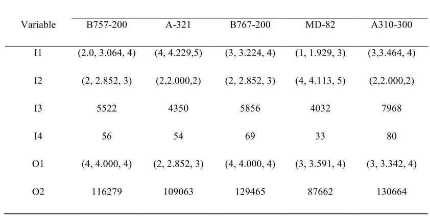
To illustrate the fuzzy DEA approach, we consider data given in Yeh and Chang 318
(2009) which was presented for an aircraft selection problem. Five types of aircraft 319
(B757-200, A-321, B767-200, MD-82, and A310-300) are to be evaluated. Four 320
inputs and two outputs are introduced in Table 5 as follows: 321
Table 5: Inputs and outputs for aircrafts evaluation
322
Data Description
Input1 (I1) Maintenance requirements (Subjective assessment)
Input2 (I2) Pilot adaptability (Subjective assessment)
Input3 (I3) Maximum range (Kilometer)
Input4 (I4) Purchasing price (US millions)
Output1 (O1) Passenger preference (Subjective assessment)
Output2 (O2) Operational productivity (Seat-kilometer per hour)
323
The first input is the aircraft maintenance capability (I1) which is concerned with the 324
availability and the level of standardization of spare parts and post-sale services. 325
The second input, pilot adaptability (I2) is related to the skills of available pilots and 326
the specific features of the aircraft. Increasing pilot adaptability and maintenance 327
capability will increase the outputs, so they are considered as inputs. To consider a 328
datum (data) as an input we should look at the effect of the datum in producing 329
On the other hand for the outputs, passengers’ preference (O1) reflects the social 334
responsibility of the airline in order to establish a positive image in public and of the 335
requirements imposed by various environment protection laws and regulations 336
whilst operational productivity (O2) is determined by the number of seats available, 337
the load rate, the travel frequency, and the aircraft travel speed. 338
In this research, the eight decision makers stated their opinion about 3 subjective 339
inputs and outputs. They used a set of five linguistic terms {very low, low, medium, 340
high, very high} which are associated with the corresponding numbers 1, 2, 3, 4 and 341
5, respectively, as in a 5-point Likert scale. 342
Table 6 shows the inputs and outputs of the five aircrafts. For example, B757-200 343
type of aircraft has two subjective inputs (I1 and I2) and one subjective output (O1), 344
with triangular fuzzy numbers. For other two inputs and one output, the values are 345
[image:20.612.109.530.412.625.2]crisps. 346
Table 6: Data for numerical example
347
DMU
Variable B757-200 A-321 B767-200 MD-82 A310-300
I1 (2.0, 3.064, 4) (4, 4.229,5) (3, 3.224, 4) (1, 1.929, 3) (3,3.464, 4)
I2 (2, 2.852, 3) (2,2.000,2) (2, 2.852, 3) (4, 4.113, 5) (2,2.000,2)
I3 5522 4350 5856 4032 7968
I4 56 54 69 33 80
O1 (4, 4.000, 4) (2, 2.852, 3) (4, 4.000, 4) (3, 3.591, 4) (3, 3.342, 4)
O2 116279 109063 129465 87662 130664
348
1.8520 and is ranked first, whilst B767-200 gives lowest score of 1.0949 and is 351
ranked last. 352
Table 7: The rank of five types of aircrafts
354
DMU h* Eff. scores Rank
B757-200 0.6348 1.2696 2
A-321 0.9798 1.1720 3
B767-200 1.0000 1.0949 5
MD-82 0.9260 1.8520 1
A310-300 1.0000 1.1237 4
6. Discussion 355
According to Theorem 2, if the objective functions corresponding to membership 356
functions in Model (5) are ignored, the optimal solution for inputs and outputs will 357
beat the endpoints of the interval of fuzzy numbers. Furthermore, if the last 358
objective function (
1
max
=
∑
s
r rp r
u y ) in Model (5) is eliminated, Lemma 1 adopted the 359
optimal solution will be in the mean value of fuzzy number. Figure 1 illustrates the 360
above mentioned concept for evaluatingDMUP. This figure can also be seen in 361
Zerafat Angiz et al. (2012). Since the discrete approach (Zerafat Angiz et al., 2012) 362
assumes the defuzzified points as its goal, so the interpretation presented in Zerafat 363
Angiz et al. (2012) is not appropriate for this specific application. The interior 364
arrows represent the optimal solution when the last objective function (
1
max
=
∑
s
r rp r
u y
365
) is absent in Model (5) and the arrows located under fuzzy numbers construct the 366
optimal solution Model (5) when only the objective function (
1
max
=
∑
s
r rp r
u y ) is 367
present. 368
370 371 372
Figure 1: Concepts of evaluating DMUs
373
Interaction between the objective functions corresponding to objective functions and 374
the last objective function (
1
max
=
∑
s
r rp r
u y ) in Model (5), cause the fuzzy optimal 375
solution. 376
7. Conclusion 377
In evaluating DMUs under uncertainty several fuzzy DEA models have been 378
proposed in the literature. The α-cut approach is one of the most frequently used 379
models. However, due to the nature of the α-cut approach the uncertainty in inputs 380
and outputs is effectively ignored. This paper has proposed a multi-objective fuzzy 381
DEA model to retain fuzziness of the model by maximizing the membership 382
function of inputs and outputs. In the proposed method, both the objective functions 383
and the constraints are considered fuzzy. A numerical example is used to show the 384
difference between the proposed and the current fuzzy DEA models. For further 385
studies, it is suggested that an exploration be done on: a) reducing the size of the 386
converted (crisp equivalent) problem, b) possible linearization of the nonlinear 387
model. 388
Acknowledgment 389
This study was supported by Universiti Utara Malaysia. We wish to thank 390
Universiti Utara Malaysia for the financial support. The funder had no role in study 391
References 395
Banker, R. D., Charnes, A., & Cooper, W. W. (1984). Some models for estimating 396
technical and scale inefficiencies in data envelopment analysis. Management 397
Science, 30(9), 1078–1092. 398
Charnes, A., Cooper, W. W., & Rhodes, E. (1978). Measuring the efficiency of 399
decision making units. European Journal of Operational Research, 2(6), 429– 400
444. doi:10.1016/0377-2217(78)90138-8 401
Emrouznejad, A. (2003). An alternative DEA measure: a case of OECD countries. 402
Applied Economics Letters, 10(12), 779–782. 403
Emrouznejad, A., & De Witte, K. (2010). COOPER-framework: A unified process 404
for non-parametric projects. European Journal of Operational Research, 405
207(3), 1573–1586. 406
Emrouznejad, A., Parker, B. R., & Tavares, G. (2008). Evaluation of research in 407
efficiency and productivity: A survey and analysis of the first 30 years of 408
scholarly literature in DEA. Socio-Economic Planning Sciences, 42(3), 151– 409
157. 410
Emrouznejad, A., Tavana, M., & Hatami-Marbini, A. (2014). The State of the Art in 411
Fuzzy Data Envelopment Analysis. In A. Emrouznejad & M. Tavana (Eds.), 412
Performance Measurement with Fuzzy Data Envelopment Analysis SE - 1 413
(Vol. 309, pp. 1–45). Springer Berlin Heidelberg. doi:10.1007/978-3-642-414
41372-8_1 415
Guo, P., & Tanaka, H. (2001). Fuzzy DEA: a perceptual evaluation method. Fuzzy 416
Sets and Systems, 119(1), 149–160. 417
Hougaard, J. L. (2005). A simple approximation of productivity scores of fuzzy 418
production plans. Fuzzy Sets and Systems, 152(3), 455–465. 419
Jain, S., Triantis, K. P., & Liu, S. (2011). Manufacturing performance measurement 420
Kao, C., & Liu, S.-T. (2000). Fuzzy efficiency measures in data envelopment 423
analysis. Fuzzy Sets and Systems, 113(3), 427–437. 424
Lábaj, M., Luptáčik, M., & Nežinský, E. (2014). Data envelopment analysis for 425
measuring economic growth in terms of welfare beyond GDP. Empirica, 41(3), 426
407–424. doi:10.1007/s10663-014-9262-2 427
Lai, Y.-J., & Hwang, C.-L. (1992). Fuzzy Mathematical Programming. In Fuzzy 428
Mathematical Programming SE - 3 (Vol. 394, pp. 74–186). Springer Berlin 429
Heidelberg. doi:10.1007/978-3-642-48753-8_3 430
León, T., Liern, V., Ruiz, J. L., & Sirvent, I. (2003). A fuzzy mathematical 431
programming approach to the assessment of efficiency with DEA models. 432
Fuzzy Sets and Systems, 139(2), 407–419. 433
Lertworasirikul, S., Fang, S.-C., Joines, J. A., & Nuttle, H. L. W. (2003). Fuzzy data 434
envelopment analysis (DEA): a possibility approach. Fuzzy Sets and Systems, 435
139(2), 379–394. 436
Lertworasirikul, S., Fang, S.-C., Nuttle, H. L. W., & Joines, J. A. (2003). Fuzzy 437
BCC model for data envelopment analysis. Fuzzy Optimization and Decision 438
Making, 2(4), 337–358. 439
Liu, J. S., Lu, L. Y. Y., Lu, W.-M., & Lin, B. J. Y. (2013). A survey of DEA 440
applications. Omega, 41(5), 893–902. doi:10.1016/j.omega.2012.11.004 441
Paradi, J. C., & Zhu, H. (2013). A survey on bank branch efficiency and 442
performance research with data envelopment analysis. Omega, 41(1), 61–79. 443
doi:10.1016/j.omega.2011.08.010 444
Pishvaee, M. S., & Torabi, S. A. (2010). A possibilistic programming approach for 445
closed-loop supply chain network design under uncertainty. Fuzzy Sets and 446
Systems, 161(20), 2668–2683. doi:10.1016/j.fss.2010.04.010 447
ranking of DMUs with fuzzy data. Fuzzy Optimization and Decision Making, 452
1(3), 255–267. 453
Sengupta, J. K. (1992). A fuzzy systems approach in data envelopment analysis. 454
Computers & Mathematics with Applications, 24(8), 259–266. 455
Takeda, E., & Satoh, J. (2000). A data envelopment analysis approach to 456
multicriteria decision problems with incomplete information. Computers & 457
Mathematics with Applications, 39(9), 81–90. 458
Tiemann, O., Schreyögg, J., & Busse, R. (2012). Hospital ownership and efficiency: 459
a review of studies with particular focus on Germany. Health Policy 460
(Amsterdam, Netherlands), 104(2), 163–71.
461
doi:10.1016/j.healthpol.2011.11.010 462
Torabi, S. A., & Hassini, E. (2008). An interactive possibilistic programming 463
approach for multiple objective supply chain master planning. Fuzzy Sets and 464
Systems, 159(2), 193–214. doi:10.1016/j.fss.2007.08.010 465
Wen, M., & Li, H. (2009). Fuzzy data envelopment analysis (DEA): Model and 466
ranking method. Journal of Computational and Applied Mathematics, 223(2), 467
872–878. doi:10.1016/j.cam.2008.03.003 468
Yeh, C.-H., & Chang, Y.-H. (2009). Modeling subjective evaluation for fuzzy group 469
multicriteria decision making. European Journal of Operational Research, 470
194(2), 464–473. 471
Zarafat Angiz, M., Saati, S., Memariani, A., & Movahedi, M. M. (2006). Solving 472
possibilistic linear programming problem considering membership function of 473
the coefficients. Advances in Fuzzy Sets and Systems, 1(2), 131–142. 474
Zerafat Angiz, M. L., Emrouznejad, A., & Mustafa, A. (2010). Fuzzy assessment of 475
performance of a decision making units using DEA: A non-radial approach. 476
Expert Systems with Applications, 37(7), 5153–5157. 477
39(3), 2263–2269. doi:10.1016/j.eswa.2011.07.118 481
Zimmermann, H. J. (1975). Description and optimization of fuzzy systems. 482
International Journal of General System, 2(1), 209–215. 483
Zimmermann, H. J. (1978). Fuzzy programming and linear programming with 484