Description of induced nuclear fission with Skyrme energy functionals: static potential energy surfaces and fission fragment properties

Description of induced nuclear fission with Skyrme energy functionals: Static potential energy

surfaces and fission fragment properties

N. Schunck,1_{D. Duke,}2_{H. Carr,}2_{and A. Knoll}3

1_{Physics Division, Lawrence Livermore National Laboratory, Livermore, California 94551, USA} 2_{School of Computing, University of Leeds, Leeds, United Kingdom}

3_{Argonne National Laboratory, Argonne, Illinois, USA}

(Received 11 November 2013; revised manuscript received 17 September 2014; published 6 November 2014) Eighty years after its experimental discovery, a description of induced nuclear fission based solely on the interactions between neutrons and protons and quantum many-body methods still poses formidable challenges. The goal of this paper is to contribute to the development of a predictive microscopic framework for the accurate calculation of static properties of fission fragments for hot fission and thermal or slow neutrons. To this end, we focus on the239_{Pu(n,f) reaction and employ nuclear density functional theory with Skyrme energy densities.} Potential energy surfaces are computed at the Hartree-Fock-Bogoliubov approximation with up to five collective variables. We find that the triaxial degree of freedom plays an important role, both near the fission barrier and at scission. The impact of the parametrization of the Skyrme energy density and the role of pairing correlations on deformation properties from the ground state up to scission are also quantified. We introduce a general template for the quantitative description of fission fragment properties. It is based on the careful analysis of scission configurations, using both advanced topological methods and recently proposed quantum many-body techniques. We conclude that an accurate prediction of fission fragment properties at low incident neutron energies, although technologically demanding, should be within the reach of current nuclear density functional theory.

DOI:10.1103/PhysRevC.90.054305 PACS number(s): 21.60.Jz,24.75.+i,25.85.Ec,27.90.+b

I. INTRODUCTION

The accurate description of neutron-induced fission is particularly important to address present challenges in the areas of energy production, nuclear waste disposal, or national security applications. Many of these applications require a detailed knowledge of fission fragment properties such as their charge, mass, and relative yields, their total kinetic energy, their total excitation energy, etc. The fission spectrum, i.e., the number and characteristics of both pre- and post-scission neutrons and gammas, often needs to be known within a few percent accuracy. In many fissile or fissionable nuclei of interest, experimental measurements are not possible, and theoretical simulations of the fission process are therefore necessary.

The central idea in the theoretical description of induced fission remains that of Bohr and Wheeler [1]: fission is modeled as a two-step process where the incident neutron first fuses with the target to form a compound nucleus (in an excited state), which then breaks into two or more fragments. These fragments will themselves decay to their respective ground states. Based on this hypothesis, powerful toolkits have been developed over the years to reproduce fission data: Monte Carlo schemes are used to simulate the deexcitation of fission fragments after scission [2–8]; reaction models focus on explaining the characteristic features of the fission spectrum such as fission isomers, collective structures, resonances, etc. [9]; nuclear structure models provide basic information on the fission fragments and the fission process itself, such as fission barrier heights, charge, mass, and energy distributions. Many results have been obtained using the macroscopic-microscopic approach to nuclear structure [10,11] and its dynamical extensions using either the general Langevin equations [12,13] or their restriction to Brownian motion [14,15]. This approach

is complemented by various scission point models, the goal of which is to simulate the actual breakup of the nucleus at large elongations [16].

This semiphenomenological framework has been very successful in explaining and reproducing numerous features of the fission process; see, e.g., Refs. [14,15,17–20] for recent applications. Nevertheless, a truly predictive theory of fission should ultimately be based on a detailed account of the nuclear forces between protons and neutrons combined with the use of standard many-body methods of quantum physics. In principle, several approaches can meet these requirements. For example, functional integral methods are fully quantum-mechanical approaches that include quantum dissipation and fluctuations [21,22]. Their implementation, however, requires computing resources that far exceed those available to the current generation of supercomputers. On paper, nuclear density functional theory (DFT) represents an excellent compromise between microscopic content and actual feasibility. In particular, DFT lends itself particularly well to separating nuclear excitations into fast intrinsic and slow collective excitations [23,24]. This distinction is especially useful in the context of low-energy nuclear fission, which has timescales of the order of 10−19_–10−20 _{seconds, i.e. two to} three orders of magnitude slower than typical single-particle excitations. Such a separation is the central assumption of the time-dependent generator coordinate method (TDGCM), which provides an effective, quantum-mechanical method to compute fission fragment yields [25–28].

the theory, such as the use of small model spaces, schematic interactions, or a reduced number of collective variables. It is only recently that the first systematic, large-scale, and accurate simulations of nuclear fission have been made possible. Most recent efforts have focused on spontaneous fission in actinide and superheavy nuclei, and quantities such as barriers and lifetimes; see, e.g., Refs. [29–36] for a selection of recent results. In contrast, there have been comparatively fewer publications on the topic of induced fission [27,28,37–39].

This paper focuses on the microscopic description of induced fission within the framework of nuclear density functional theory with Skyrme energy densities. As such, it should be considered as an intermediate step in the long-term effort to achieve a predictive theory of fission. The specific goals of this paper are (i) to provide a comprehensive mapping of deformation properties of 240_{Pu, (ii) to give a detailed} and quantitative analysis of the role of triaxiality in fission calculations, (iii) to assess the dependence of calculations on the parametrization of the functional, and (iv) to establish a template for the calculation of fission fragment properties. In several aspects, this study is both a continuation and an exten-sion of the general description of induced fisexten-sion developed over the years at the Commissariat `a l’Energie Atomique in France and Lawrence Livermore National Laboratory in the USA; cf., for example, Refs. [25–28,37–45].

SectionIIcontains a brief reminder of the nuclear density functional approach to induced fission, Skyrme functionals, and the practical implementation of DFT. SectionIIIfocuses on the static potential energy surfaces in 240Pu, which is the compound nucleus formed in 239_{Pu(n,f), and their} dependence on the parametrization of the Skyrme and pairing functionals. Section III D presents a detailed analysis of the identification of the scission point based both on topological methods and the concept of quantum localization, and provides estimates of fission fragment properties for the most probable fission.

II. THEORETICAL FRAMEWORK

Our theoretical approach is based on the local density approximation of the energy density functional (EDF) theory of nuclear structure. The next few sections review the basic ingredients of the EDF theory pertaining to the description of nuclear fission.

A. Density functional theory approach to induced fission In the context of nuclear fission, the ultimate goal of nuclear density functional theory is to provide a comprehensive and accurate description of both the fissioning nucleus (half-lives, fission probability) and the fission fragments (mass and charge distributions, excitation energy, yields, etc.) based on the best knowledge of nuclear forces and quantum many-body techniques.

Density functional theory of nuclei is a mature field with numerous applications in low-energy nuclear physics and nuclear astrophysics [24,46]. The central assumption of the approach is that atomic nuclei can be described accurately by an effective energy density H, which is a functional of the

one-body density matrix and the pairing tensor—since pairing correlations play an essential role in low-energy nuclear structure. This energy density may or may not be derived from an effective pseudopotential ˆVeff. In practice, most applications of DFT so far have used either the Skyrme or Gogny energy density, which are indeed derived from an effective two-body pseudopotential, of zero range for Skyrme and finite range for Gogny. The coupling constants of the energy density are free parameters to be determined, usually on global observables such as atomic masses, r.m.s. radii, nuclear matter properties, etc.; See, e.g., Refs. [47–49] for recent applications.

For the specific case of induced fission, two additional hypotheses underpin the DFT approach:

(1) One can identify a set of collective degrees of freedom q that drive the dynamics of the fission process. The most important of these collective degrees of freedom are related to the nuclear shape, although additional collective variables related, e.g., to the pairing channel, could be introduced [29]. The collective degrees of freedom might be considered as free parameters of the theory, although the variational nature of DFT ensures that the more collective variables there are, the better the accuracy is.

(2) The transition between the compound nucleus and fully independent fission fragments can be controlled by the introduction of scission configurations. Without this additional constraint, the short range of nuclear forces combined with the variational nature of DFT would always yield fission fragments in their ground-state configurations, so that the total energy of the system be minimal. This is contrary to experimental data, which shows that fission fragments can be excited.

We note that these two assumptions are reminiscent of semiphenomenological approaches to fission, in partic-ular scission point models using inputs from macroscopic-microscopic potential energy surfaces [16]. The main dif-ference is that DFT is built onto a unique energy density that simultaneously determines bulk and shell effects, the collective inertia, and the dynamics of the problem in a unifying quantum-mechanical framework.

Based on the aforementioned hypotheses, the full DFT description ofinducedfission relies on the following multi-step approach:

(1) Static properties of the fissioning nucleus are computed as a function of the collective degrees of freedom q. These potential energy surfaces are obtained by solving the DFT equations, which most often take the form of the Hartree-Fock-Bogoliubov equations with constraints. This step can be viewed as the construction of an adequate basis made of those nuclear many-body states that are the most relevant for the fission process. (2) Scission configurations are then identified on the potential energy surface, based on some criteria. It is precisely the purpose of this paper to discuss in details some of these criteria.

under the general assumptions of DFT, namely that the ground state takes the form of a Slater determi-nant (HF) or, when pairing correlations are included, of a quasiparticle vacuum (HFB). This could be done “directly” with the time-dependent Hartree-Fock (TDHF) theory, and its extension with pairing, the time-dependent Hartree-Fock-Bogoliubov (TDHFB) theory [50,51]. Alternatively, one may use the basis of many-body states generated in step 1 to formulate a collective, time-dependent, Schr¨odinger-like equation: this is the essence of the time-dependent generator coordinate method (TDGCM) [40–42]. In practice, only the TDGCM has been applied to the study of fission fragment distributions so far [25–28,45].

One should emphasize that, strictly speaking, the DFT description of fission requiresallof the aforementioned steps. In particular, while potential energy surfaces can provide valuable inputs to reaction models, or even be used to compute pseudoexperimental quantities such as fission barriers, they are, in reality, only an auxiliary basis used to compute the fission fragment properties in the TDGCM. In this paper, the focus is on selected topics pertaining to thestaticaspects of fission. We leave the calculation of fission fragment properties, yields, and distributions to a forthcoming paper.

B. Skyrme energy functional

In the local density approximation of the EDF theory, the energy of the nucleus is given as the integral over space of the Hamiltonian densityH(r), which is itself a functional of the one-body density matrixρand pairing tensorκ,

E=

d3rH(r). (1)

The Hamiltonian density is built out of a kinetic energy density term, a potential energy densityχt, and a pairing energy density

˜ χt:

H[ρ,κ]= 2 2mτ(r)+

t₌0,1 χt(r)+

t₌0,1 ˜

χt(r), (2)

whereτ(r) is the kinetic energy density, and the indextrefers to the isoscalar (t=0) or isovector (t =1) component of the potential energy density; see Ref. [52] and references therein. In this work, the potential energy density is obtained from the zero-range Skyrme pseudopotential [53]. We employed three different parametrizations of the Skyrme EDF: (i) The SkM* parametrization [54] remains a standard in fission calculations with Skyrme EDFs; see, e.g., Refs. [30,31,35,36,55–58] for some recent applications. Since the parameters of the pseudopotential were explicitly adjusted to fission barrier heights, it is believed to have good deformation properties. (ii) The UNEDF0 EDF is a recent parametrization of the Skyrme energy density that gives a very good agreement with nuclear masses [47] but was shown to have unrealistic deformation properties [48,59]; we use it only to study the impact of model parameters on fission observables. (iii) The UNEDF1 EDF was obtained by extending the optimization protocol of UNEDF0 to include selected data on fission isomers [48].

It offers an excellent compromise between predictive power (limited amount of data used in the fit) and overall quality.

In this work, pairing correlations are treated at the Hartree-Fock-Bogoliubov (HFB) approximation [60]. The pairing energy density ˜χ is a functional of the pairing tensorκ, or equivalently of the pairing density ˜ρ [24]. It is derived from a density-dependent contact pairing interaction with mixed volume-surface character [61],

ˆ

Vpair(r,r)=V0(n,p)

1−1 2

ρ(r) ρc

δ(r−r), (3)

withV₀(n,p) the pairing strength for neutrons (n) and protons (p), andρc=0.16 fm−3 the saturation density. The energy cutoff was set at Ecut=60 MeV. For our calculations with the SkM* EDF, we adjusted V₀(n) and V₀(p) locally on the three-point odd-even mass difference in 240_{Pu. This gave} V₀(n) = −265.25 MeV andV₀(p) = −340.06 MeV. In the case of UNEDF0 and UNEDF1, the value of the pairing strengths V₀(n,p)is fixed by the parametrization; in addition, calculations with these two functionals are performed using an approximate formulation of the Lipkin-Nogami prescription [46,62].

The nuclear shape is characterized by the expectation value qλμ of the multipole moment operators ˆQλμ on the HFB vacuum. We will also employ the expectation value of the so-called Gaussian neck operator,

ˆ

QN =e−(

z−zN aN )

2

, (4)

which gives an estimate of the number of particles in the region centered around the pointzN [38,63,64]. We chose the range aN=1.0 fm. The collective space of nuclear fission is defined as the ensemble of constraints imposed on the HFB solution. In this work, we will consider the following constraints, either alone or in combinations: elongation ˆQ₂₀, degree of triaxiality ˆQ22, mass asymmetry ˆQ30, neck thickness ˆQ40, and neck size ˆQN. These collective variables will be denoted generically byq =(q1, . . . ,qN). Constrained HFB solutions are obtained by using a variant of the linear constraint method, in which Lagrange parameters are updated based on the cranking approximation of the random phase approximation (RPA) matrix [38,65,66].

C. DFT solver and numerical precision

All calculations were performed with the DFT solvers

HFODD[66] andHFBTHO[67]. Both solvers implement the HFB equations with Skyrme functionals in the one-center harmonic oscillator (HO) basis. The programHFBTHOassumes axial and time-reversal symmetry, whileHFODDbreaks all symmetries.

In Cartesian coordinates, the three-dimensional HO basis is characterized by its frequencyω₀3=ωxωyωz, the maximum oscillator numberNmax, the total number of basis statesNstates, and the deformation β2, which accounts for the different frequencies in each Cartesian direction.

imposed by the physical limits on the memory available and CPU time taken by the calculations.

At the large elongations encountered in the description of fission, the truncation of the HO model space results in a strong dependence of the HFB calculations on the basis frequency and deformation. Based on several experiments, we assume the oscillator frequency ω0 and basis deformation β2 vary with the requested expectation value q20 of the axial quadrupole moment ˆQ20according to

ω0=

0.1×q₂₀e−0.02q20+_{6.5 MeV if}|_q

20|30 b, 18.14 MeV if|q20|>30 b, (5) and

β =0.05√q₂₀. (6)

This choice largely mitigates basis truncation effects up to the scission point, where we empirically estimate the error on the total energy to be of the order of 2–3 MeV [68].

From the estimates given above, it should be clear that accurately capturing the physics of fission with one-center bases is extremely challenging. Recent studies of convergence properties in the HO basis have pointed to the existence of more reliable extrapolation methods [69,70]. Translating these results in the context of DFT may not be straightforward: contrary to the ab initioapproach, the effective Hamiltonian of Skyrme EDFs depends on the density, hence on the model space. The alternatives to the one-center HO basis all have limitations of their own. Codes using the two-center HO basis [27,39,40], where basis functions must be reorthogonalized, or the coordinate-space representation of quasiparticle wave-functions [71] do not currently include triaxiality. Lattice rep-resentations generate large amounts of data [72]. A promising alternative based on multi-resolution wavelet representation of HFB wave-functions [73] remains in its infancy and may incur a high cost of a single HFB calculation. As we progress in our understanding of fission mechanisms, however, it will become more and more necessary to improve the numerical precision of DFT solvers.

III. STATIC DEFORMATION PROPERTIES OF240_Pu In this section, we discuss the features of the static potential energy landscape of 240_{Pu. In particular, our goals are to} (i) discuss and highlight the role of several shape collective variables, (ii) assess more specifically the effect of triaxiality on the barriers and beyond scission, and (iii) quantify the effect of the parametrization of the energy density on predictions of static fission pathways.

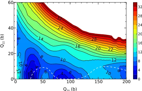
A. Overview of the potential energy surface of240_Pu We begin by presenting a set of two-dimensional potential energy surfaces (PESs) that provide useful information on the local topography of the total energy in the four-dimensional collective space introduced at the end of Sec.III C 1. In Fig.1, we plot the total HFB energy as a function of the quadrupole degrees of freedom in the vicinity of the ground state (g.s.) and the fission barriers. In this calculation, the octupole moment was set to 0 (symmetric path), and the hexadecapole

0 50 100 150 200 Q₂₀(b)

0 20 40 60

Q22

(b)

2 4

4 6

6 8

8 8

8

10 10

10

12

12 14

16 8

20 22

24

28 30

32

0 4 8 12 16 20 24 28 32

FIG. 1. (Color online) Two-dimensional potential energy surface of240_{Pu in the (q}

20,q22) plane for the SkM* EDF. The energy is relative to the ground-state value. The dashed line represents the symmetric, triaxial least-energy pathway.

moment was left unconstrained. The ground state, (q20,q22)≈ (35 b,0 b), and fission isomer, (q20,q22)≈(80 b, 0 b), are clearly visible, as well as the lowering of the first fission barrier owing to triaxiality. Although less visible in the contour map, the second barrier is also slightly triaxial. We will quantify the effect of triaxiality on the least-energy fission pathway in more detail in Sec.III B.

Next, we show in Fig.2 the potential energy surface in the (q20,q40) plane. The well-known fusion (in the right-hand side of the figure) and fission (in the left-hand side) valleys are clearly visible. We note that the barrier between the two valleys is smaller in our Skyrme SkM* calculations than, e.g., for the Gogny D1S functional [38]. For the hot fission process, the least-energy fission pathway starts from the g.s. and follows the fission valley until the barrier between the fission and fusion valleys vanishes.

Finally, we probe the mass asymmetry degree of freedom. In Fig.3, we show the potential energy surface in the (q20,q30) plane. Since the fission fragment mass distribution of240Pu

200 250 300 350 400 Q₂₀(b)

40 60 80 100 120 140 160

Q40

(b

2)

4

6 8

10

12

20

22 24

26

28 28 30

32

34

36 8

2

42

46

0 6 12 18 24 30 36 42 48

Fission V alley

Fusion V alley

FIG. 2. (Color online) Two-dimensional potential energy surface of240_{Pu in the (q}

0 100 200 300 400 500 600 Q₂₀(b)

0 10 20 30 40 50 60

Q30

(b

3

/

2)

0

4

8

12

16

20 24

28

32

36

40 ₄₀

40

44

44

44 48

52

56 56

60

64 64

68

68 72

76

0 8 16 24 32 40 48 56 64 72

FIG. 3. (Color online) Two-dimensional potential energy surface of240_{Pu in the (q}

20,q30) plane for the SkM* functional. The energy is given relative to−1840 MeV. The dashed line represents the least-energy pathway.

is known to be asymmetric, this degree of freedom is among the most important for a quantitative description of induced fission. This calculation is by far the largest, as we have to cover all the collective space from symmetric fission (up toq20 ≈ 550 b to highly asymmetric fission (up toq30≈70 b3/2). In addition, accurate prediction of the fission fragment properties (charge and mass distributions, kinetic energies, etc.) requires the good identification of the scission region, hence a relatively dense mesh.

The figure shows the least-energy fission pathway, which goes from aboutq20≈100 b andq30=0 b3/2and exits near q₂₀ ≈345 b andq₃₀=40 b3/2_{. We note that there is another} fission valley that starts directly from the ground state and exits at small elongation but a very large asymmetry of about q30 >60 b3/2. This exotic, very asymmetric, fission channel corresponds to cluster radioactivity and was discussed recently in Ref. [33].

We also emphasize that the PES of Fig.3 exhibits clear signs of discontinuities, especially (but not exclusively) in the region 300< q20 <550 b andq30≈20 b3/2. As discussed in detail in Ref. [44], these discontinuities are the consequence of using the self-consistent procedure in a truncated collective space of finite size: only a limited number of collective variables are explicitly constrained, which produces these numerical artifacts. Such discontinuities, however, provide also great physical insight since they “automatically” signal where collective degrees of freedom are missing for the proper description of the process.

B. Fission pathway of least energy

From this section on, we will focus exclusively on the least-energy fission pathway. It is defined as the pathway connecting the ground state to the point of scission, along which the energy remains a local minimum in the full collective space. It was shown recently that the dynamic fission pathway, as obtained from the minimization of the collective action together with the proper treatment of the collective inertia, is very close to the least-energy pathway [74]. The latter is, therefore, a good approximation of the most probable fission path.

0 100 200 300 400 500 600 Q20(b)

-8 -4 0 4 8 12 16

HFB Energy (MeV)

0 50 100 150 200 250 300 350

Multipole Momen

t

Q0

(10

fm

)

Q40

(symmetric)

Q₄₀(asymmetric)

Q₃₀(asymmetric)

FIG. 4. (Color online) Energy along the least-energy fission path-way in240_{Pu for the SkM* EDF: axial symmetric path (black squares),} triaxial symmetric path (red circles), and triaxial asymmetric path (blue triangles). Energy curves are given relative to the ground state. The value of the octupole and hexadecapole moments are also shown along the symmetric and asymmetric paths.

In Fig. 4, we superimpose the energy along the least-energy least-energy fission pathway in three different scenarios: (i) symmetric (q30=0 b3/2) fission with no triaxiality (q22= 0 b, or γ =0o_{), (ii) symmetric fission with triaxiality, and} (iii) asymmetric fission with triaxiality. In scenario (ii), we introduced a constraint on the expectation value of ˆQ22during the first few iterations of the self-consistent procedure, before completely releasing this constraint: this enabled the nucleus to jump into a triaxial region in the case there would have been a small barrier between the axial and triaxial solutions; finally, in scenario (iii), the same methodology was repeated for the octupole degree of freedom ˆQ30.

It is well known that including triaxiality lowers the first barrier [75–77]. It also lowers the second barrier, but only along the symmetric fission path. We find that the degree of triaxiality is large at the first barrier,γ ≈32oand remains significant in the second barrier, γ ≈15o. As seen from Fig. 4, the first barrier is lowered by approximately 2 MeV when triaxiality is included. We note that both the octupole and hexadecapole moments vary relatively smoothly along the path.

A clear deficiency of the SkM* functional is that the first fission barrier height is EA≈7.64 MeV, which is about 1.6 MeV higher than the empirical barrier [78,79]. However, predictions of SkM* are in the same region as those of competing models [30]. In addition, the experimental uncertainty for the fission barrier (which is not an observable) is usually estimated to be of the order of 1 MeV. One should, therefore, be satisfied with an overall reproduction of barriers within 1–2 MeV of the empirical value. Similarly, the fact that the one-neutron separation energy of 240_{Pu computed} with SkM* is Sn=7.04 MeV, which is lower than the top of the barrier and (unrealistically) implies that 239_{Pu is not} fissile, should not be a cause of special concern because of the uncertainties on the fission barriers.

FIG. 5. (Color online) Variation of the total HFB energy as a function of the hexadecapole moment q40 along the least-energy fission pathway in240_Pu.

pathway is truly the lowest-energy path connecting the ground state to the scission point, at least within the numerical accuracy of the calculations. In particular, we verify a posteriori in Fig.5 the correctness of the calculation in the scission region by showing cross sections of the energy as a function of the hexadecapole moment at several points along the path. Together with the two-dimensional PES of Fig.2, it confirms that our least-energy fission pathway stays within the fission valley, and, therefore, corresponds as expected to the hot fission process.

C. Dependence on the energy functional

Previous studies carried out with the finite-range Gogny pseudopotential and the D1S parametrization showed that symmetric fission occurs at very large values of the quadrupole moment, around q20 ≈590 b [38]. We report qualitatively similar results with the Skyrme SkM* parametrization, al-though the actual value of the quadrupole moment is signifi-cantly lower, aroundq20≈550 b. Similarly, the hot scission point for asymmetric fission is located around (q30,q40)≈ (64 b3/2_{,187 b}2_{) for the Gogny D1S, while it is (q}

30,q40)≈ (40 b3/2_{,136 b}2_{) for the SkM* parametrization. Since we have} verified that the one-dimensional fission pathways reported earlier are truly at the bottom of the fission valley (see previous section), it is highly unlikely that the differences observed between D1S and SkM* originate from numerical or algorithmic errors. Instead, they should be attributed to the intrinsically different deformation properties of each EDF. In this section, we explore the sensitivity of both the full fission pathway and the position of the scission configurations on the form of the energy density used.

1. Dependence on the Skryme energy density

To investigate further the dependence of the scission point on the parametrization of the energy functional, we have computed the least-energy fission pathway with the UNEDF0 [47] and UNEDF1 functionals [48]. Benchmarks of fission barriers and fission isomer excitation energies were already

0 100 200 300 400 Q₂₀(b)

-10 -5 0 5 10 15

HFB Energy (MeV)

SkM* UNEDF0 UNEDF1

FIG. 6. (Color online) Energy along the least-energy fission path-way in240_{Pu for three parametrizations of the Skyrme functional:} SkM* [54], UNEDF0 [47] and UNEDF1 [48]. All curves are given relative to their ground-state value.

reported and discussed in Refs. [30,48]. Here, we push the calculation up to the scission point and beyond. In this section, scission is simply defined as the occurrence of a sharp discontinuity in the PES before which the nucleus is whole (qN 1), and after which it is made of two fragments (qN 1). The energy along the least-energy fission path is shown in Fig. 6, and the position of the scission point is summarized in TableI.

Interestingly, the position of the scission point is nearly the same for UNEDF0 and UNEDF1, even though the pre-scission energy (difference between the potential energy at the top of the second barrier and at scission) is remarkably different, with approximately 12.5 MeV for UNEDF1 and only 3.4 MeV for UNEDF0. These differences in deformation energy are especially striking since these two functionals give very similar results across a broad range of nuclear observables including atomic masses, radii, odd-even mass differences, neutron droplets, etc.. They are most likely caused by the large difference in the surface-symmetry energy between the two functionals,assym = −44 MeV for UNEDF0 andassym =

−29 MeV for UNEDF1, which decreases significantly surface tension effects [59].

2. Dependence on the pairing strength

One trademark of the UNEDF family of Skyrme functionals is that the two pairing strengths of the functional (3) are

TABLE I. Approximate position of the scission point in the (q20,q30,q40) plane for the three parametrizations of the Skyrme functionals: SkM*, UNEDF0 and UNEDF1.

Functional Qˆ20(b) Qˆ30(b3/2) Qˆ40(b2)

SkM* 345 43 136

UNEDF0 354 44 144

0 100 200 300 400 Q₂₀(b)

-5 0 5 10

HFB Energy (MeV)

90% Pairing 95% Pairing 100% Pairing 105% Pairing 110% Pairing

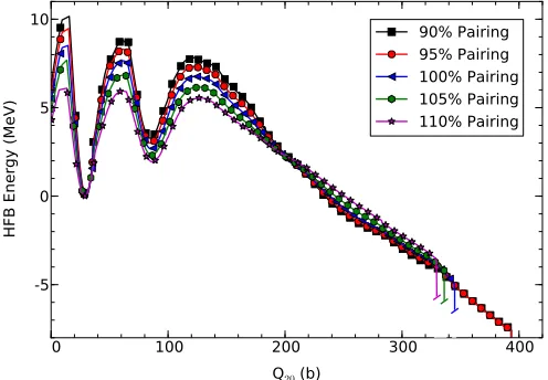
FIG. 7. (Color online) Energy along the least-energy fission path-way in240_{Pu for five parametrizations of the pairing force and the} SkM* parametrization of the Skyrme functional. All curves are given relative to their ground-state value.

fitted simultaneously with the coupling constants of the Skyrme functional, i.e., the particle-hole and particle-particle channels of the EDF are treated on the same footing. In addition, these functionals are used with an approximate formulation of the Lipkin-Nogami prescription to limit the fluctuations in particle number. The different fission pathways and scission configurations reported in the previous section could, therefore, be attributed either to the Skyrme functional itself, to the pairing channel, or to a complex interplay between the two. In this section, we briefly analyze the role of pairing correlations alone.

In Fig.7, we have performed additional calculations of the fission pathway in 240_{Pu by varying both pairing strengths} V₀(n) andV₀(p) by−10%,−5%,+5%, and+10%. Variations of ±5% of the pairing strength lead to variations of about 250 keV of the pairing gaps computed in the g.s. This value is often taken as an estimate of the predictive power of surface-volume pairing interaction combined with Skyrme functionals to reproduce odd-even mass differences [80].

The effect of pairing correlations on fission barrier and collective inertia is well known; see, e.g., [81] and references therein. Less known is the impact of pairing correlations on the scission point. We find that increasing pairing decreases the value of the quadrupole moment where scission occurs. Conversely, decreasing pairing moves the scission configura-tions to larger quadrupole moments. The effect is particularly pronounced if pairing correlations vanish: for pairing strengths decreased by both 5% and 10%, neutron pairing correlations are 0 beyondq₂₀ >238 b, resulting in a shift of the scission point by nearly 50 b compared to the original calculation. This result suggests that a predictive theory of nuclear fission based on DFT will require a very accurate description of pairing correlations.

D. Scission region

By contrast to current theories of spontaneous fission, which rely on the detailed knowledge of the potential energy

FIG. 8. (Color online) Two-dimensional potential energy surface of240_{Pu in the (q}

20,q22) plane for the SkM* functional around the least-energy fission pathway. The energy is normalized arbitrarily at

−1820 MeV.

surface only in the vicinity of the ground state and the two fission barriers, models of induced fission need to describe the collective space up to, and beyond, the point of scission. Below, we discuss some of the features of the PES in the scission region for240Pu.

1. Triaxiality at and beyond scission

While the impact of triaxiality on fission barriers has been established for over forty years, little else is known about the role of this degree of freedom in the fission process. The additional cost of breaking axial symmetry is significant, both computationally and physically (loss of theK quantum number). The purpose of this section is to highlight the role of triaxial shapes at scission and beyond.

We show in Fig.8the potential energy of240Pu for the SkM* functional in the (q20,q22) plane near scission. Calculations are based on the least-energy fission pathway of Fig.4. For each point in the (q20,q22) mesh of Fig. 8, the HFB calculation is initialized with the nearest HFB solution along the least-energy fission pathway, with the additional condition that the initial solution satisfiesq20 <300 b. The purpose of this last condition is to ensure that the initial guess for the HFB solution corresponds to a whole nucleus and not two fragments. The resulting map can be interpreted as a local two-dimensional cross section in the (q20,q22) along the least-energy fission pathway.

FIG. 9. (Color online) One-dimensional potential energy surface of240_{Pu along theq}

22direction for the SkM* functional around the least-energy fission pathway.

fission fragment properties as they shift the scission point to lower elongations: TableIIlists the average proton and neutron numbers of the fission fragments at the triaxial scission points. There is a variation of about 0.5 proton and 1 neutron across this region.

The modification of the fission fragment properties induced by triaxiality should be visible in a dynamical description of fission such as the time-dependent generator coordinate method [27,28]. The relative flatness of the collective space in the (q20,q22) plane should indeed divert a fraction of the collective flux, which will impact the relative charge and mass distributions of the fragments. In addition, we may expect a nonzero dissipation in energy in the transverse collective modes, here characterized by theq₂₂collective variable, which should reduce the available pre-scission energy [26].

2. Continuous evolution across the scission point

As discussed extensively in Ref. [38], an accurate prediction of fission fragment properties is not possible if the collective space is restricted to the (q20,q30,q40) variables; see also Sec.IV Ebelow. Including the triaxial degree of freedom does not fundamentally alter these conclusions: in such restricted collective spaces, scission still manifests itself by a sharp discontinuity of the potential energy surface. Just before this discontinuity, the pre-fragments are heavily entangled with the consequence that the calculated total kinetic energy

TABLE II. Variation of the light (L) and heavy (H) fragment proton and neutron numbers as a function of triaxiality near the least-energy fission pathway.

q20(b) q22(b) ZH NH ZL NL

310.0 7.0 53.6 84.5 40.4 61.4

320.0 6.0 53.7 84.8 40.3 61.2

330.0 5.0 53.9 85.2 40.1 60.8

340.0 4.3 54.0 85.5 40.0 60.6

FIG. 10. (Color online) Potential energy surface in the (q30,qN)

plane just before scission for the SkM* functional. The axial quadrupole moment Qˆ20 is fixed at q20=345 b, the triaxial quadrupole ˆQ22and hexadecapole moments ˆQ40are unconstrained. The energy is normalized arbitrarily at−1827 MeV.

is totally unrealistic. Just after the discontinuity, however, the fragments are neatly separated but in their ground-state: this is a consequence of the variational principle behind the HFB approach, and is in contradiction with the experimental evidence that fission fragments are excited after scission.

It is, in fact, quite simple to introduce additional collective variables that will transform the discontinuity at scission into a continuous pathway. Among the possible choices, a constraint

ˆ

QN on the density of particles in the neck between the two pre-fragments has often been used, both in the context of spontaneous fission [64], and induced fission [38]. We show in Fig.10a close-up of the local potential energy surface of 240_{Pu near the scission point for the SkM* functional. The} axial quadrupole moment is fixed atq20=345 b while the triaxial quadrupole ˆQ22 and hexadecapole moments ˆQ40 are unconstrained. Only the range [0,1] ofqNis represented, as it is in this area that the scission process seems to take place (see discussion in Sec.IV B). AtqN =1, the least-energy fission pathway emerges atq30 ≈30 b3/2. It broadens up to form a wide “estuary” in the (q30,qN) subspace: the energy surface is very shallow across a large range of octupole moments. This should manifest itself by a sizable broadening of the yields.

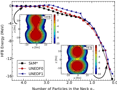
In order to better visualize the variations in energy when following this continuous path, we show in Fig. 11 the one-dimensional profile of the total energy as a function of qN for the three functionals used in this work. For each curve, the value of the axial quadrupole moment is fixed at the value just before scission as listed in TableI, and calculations are performed with a constraint on ˆQN. All other multipole moments are unconstrained. The curves are normalized at the value ofqN=4.5. It is worth noticing that the energy gain along this extra dimension in the collective space is very similar for all three functionals, even though the potential energy surface in theq20 direction can be dramatically different; see Fig.4. On average, variations ofqNlower the energy by up to 12–15 MeV.

-10 0 10 x [fm] -10

0 10

z [fm]

-1

-1

-2 -2

-3

-3 -4 -5

-6

-7

-8

-10 q =0.3

-10 -8 -6 -4 -2 0

-10 0 10

x [fm] -10

0 10

z [fm]

-1

-2 -3

-4 -5 -7

-9

10 q =4.0

-10 -8 -6 -4 -2 0

0.0 1.0

2.0 3.0

4.0

Number of Particles in the Neck q_N

-16 -12 -8 -4 0

HFB Energy (MeV)

SkM* UNEDF0 UNEDF1

FIG. 11. (Color online) Total energy as a function of the density of particles in the neckqN along the least-energy fission pathway

for the SkM*, UNEDF0, and UNEDF1 functionals. All curves are normalized relative to their respective values at qN =4.5. Inset

contour plots show the density profile atqN =4.0 andqN=0.3.

to two distinct fragments. The qN degree of freedom can, therefore, be viewed as a kind of control parameter. It can be used in several ways. The scission configurations can be chosen along the qN axis arbitrarily, on the sole basis of phenomenological comparisons with experimental data, e.g., on charge and mass distribution of fission fragments. Alternatively, additional criteria can be invoked to pin down the scission configuration at a given value ofqN, or in a given interval ofqN values. This is the approach that we chose and that we discuss in more detail in the next section.

IV. NUCLEAR SCISSION AND FISSION FRAGMENT PROPERTIES

The purpose of any theory of induced fission is to predict fragment properties such as charge and mass distribution, kinetic energy, excitation energy of each fragment, fission spectrum, etc., as these correspond to measurable quantities. In the nuclear DFT approach, computing these properties require introducing scission configurations in the compound nucleus. After a brief historical reminder, we present below the methods that we used to define the scission configurations, as well as its application in the calculation of fission fragment properties for the least-energy fission pathway of240_Pu.

A. Definition of scission

The concept of a scission point has its origin in the liquid drop (LD) picture of the nucleus and reflects the fact that for very large deformations, the LD potential energy is a mul-tivalued function of the deformation parameters [11,82,83]. These multivalues generate discontinuities in potential energy landscapes, which are still widely used as a criterion to define the scission configurations [28,35,38,39]. However, as we have recalled in the previous section, these discontinuities

are entirely spurious since locally enlarging the collective space can easily restore the continuity of the full PES [44]. In addition, continuous PESs give additional flexibility to define the scission configurations and improve the predictive power of the theory.

As mentioned above, rather than use the qN degree of freedom as a simple control parameter that we could tune to data, we would like to find general criteria, based either on mathematics and/or on physics, to define the scission configurations, and let the theory take care of the comparison with the data without further empirical adjustments. The simplest criterion one could invoke to define scission is to set a minimum value for the size of the neck,q_N(min), below which one assumes the neck is small enough that the two fragments can be considered fully formed [38,39]. Such an approach has the advantage of being easy to automate, but the choice ofq_N(min) remains entirely arbitrary. A possible extension would be to set up a range inqN values, say Iq =[qN(min),q

(max)

N ], where scission configurations are chosen, and use the boundaries of this interval as estimates of theoretical errors. Ideally, this interval should be as narrow as possible. Since at scission one connected nucleus becomes two unconnected fragments, tools based on detecting connectivity features in datasets (here the nuclear density) should be applicable, and may help in making the determination ofIq less arbitrary. We will explore this option in detail in Sec.IV B.

For the sake of completeness, we also mention an alternative strategy to identify scission configurations. It was recognized early on that the competition between the repulsive Coulomb and the attractive nuclear forces may induce the scission of the nucleus even when there still remains a sizable neck between the two nascent fragments; the ratio of the Coulomb energy over the nuclear interaction energy can, therefore, provide a complementary, dynamical, criterion for scission [84,85]. Recently, a similar approach was formalized in the context of nuclear density functional theory [37]. Two major ingredients are required: (i) the calculation of the Coulomb and nuclear interaction energies and (ii) a procedure to “localize” the fragments, since both the Coulomb and nuclear interaction energy are representation dependent; see Sec. IV D below. These approaches can of course be combined with the method we describe below.

8 9

5 6

1 2 3

4 7 6 7 8 2 3 4 4 5 6 7 5 6 7 ₈ 2 3 4

8 7 1

2 5

4

3 6 9 1

2 3 4 6 7 8 9 6 7 8 4 3 1 2 3 4 6 7 8 9 5 (a) (b)

FIG. 12. Two small functionsf(x,y) andg(x,y) on a triangular mesh (dashed lines) shown as contour plots and their respective contour trees. Circled (a) and squared (b) points represent the values of the function on the mesh.

in the physical system. In place of geometric properties, our approach draws on the mathematics of topology to derive global properties (invariants) of space. Topological analysis of data sets results in structural abstractions that can be used to answer questions of whether two spaces have fundamentally the same shape, and to articulate the types of differences that appear. In the physical sciences, topological feature analysis is well known in the study of flow (e.g., vortices, separatrices) [86–88] and in the analysis of scalar fields (e.g., critical points) [89–91]. Its main advantage is that it moves identification of phenomena from assessment against empirical, possibly subjective, thresholds into binary decisions based on change to the discrete structures that express fundamental topological properties. This leaves two questions: Which (if any) topological change in data correlate with the physical phenomena of interest, and can topological structure be computed “effectively”?

Recent work in scientific visualization and computational topology has shown how to analyze features in functions of the formf :R3→R, such as the local nuclear densityρ(r). In these functions, the connectivity of isovalued contours can be analyzed using thecontour tree [92], which captures the relationships of all possible contours in a data set. Figure12

gives a pedagogical illustration of the technique: maxima and minima of the contour map are leaves of the tree, while critical points (saddles) are interior nodes. Moreover, one characterization of critical points is that they are the highest points at which two peaks are connected. As a result, the critical points naturally define features corresponding to branches of the tree. Subsequent work showed that these features can then be tracked over time (or any other relevant parameter) [93].

While this approach works for single-valued functions, it needs modification for bivariate functions of the form (f,g) :

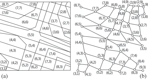
R3_→R2_{. For such a function, contours do not naturally divide} it into features, and a generalization of the contour tree is required, as shown in Fig. 13. Here, the domain is divided along contours of bothf andg, resulting in a set of regions, or “slabs,” as shown. To understand how the abstract graph of panel (b) is obtained from the original contours of panel (a), consider for instance the lower left corner of panel (a): the slab marked (3,2) is adjacent to the slabs (3,1) and (4,2). Hence, the node (3,2) is connected to the two nodes (4,2) and (3,1). Systematically analyzing the connectivity of these slabs thus gives thejoint contour net(JCN) shown in panel (b) of Fig.13: an abstract representation of the joint variation offandg[94].

(3,1) (3,2) (4,2) (5,2) (6,2) (4,3) (5,3) (6,3) (7,3) (8,3) (4,4) (5,4) (6,4) (7,4) (5,5) (3,6) (2,6)

(4,6) (6,6) (7,6) (8,7) (7,7) (6,7) (3,7) _(2,7) (7,8) (2,8) (3,1) (3,2) (4,1) (4,2)

(5,2) (6,2) (7,2) (4,3) (5,3) (6,3) (7,3) (8,3) (9,3) (4,4) (5,4) (6,4) (7,4) (5,4) (5,5) (8,4) (6,5) (4,5) (6,5) (3,5) (3,6) (2,6) (4,6) (5,6) (6,6) (7,6) (8,7) (7,7) (6,7) (5,7) (4,7) (3,7) (2,7) (6,8) (5,8) (4,8) (3,8) (2,8) (1,8) (4,9) (3,9)(2,9)_(1,9) (7,8)

(a) (b)

FIG. 13. Joint contour slabs found by intersecting the slabs of functions f and g of Fig. 12 (a). Joint contour net obtained by analyzing the connectivity of the slabs; see text for details (b).

The case of nuclear fission lends itself perfectly to such an analysis. Indeed, within nuclear DFT the nucleus is entirely characterized by the neutron (ρn) and proton (ρp) densities, which will play the role of the two distinct yet correlated scalar fieldsf andgin the example of Figs.12and13. Any special feature of the JCN graph associated with the bivariate function (ρp,ρn) :R3→R2 could therefore, in principle, be given a physical interpretation. In fact, we have recently shown that the sudden division of the compound nucleus in two separate fragments at the discontinuity of one-dimensional fission pathways E(q20) is clearly associated with a fork in the JCN [95]. Here, we extend the method to the more difficult problem of detecting features along a continuous

fission pathway characterized by theqN constraint.

Figure 14 illustrates the application of the JCN method to the detection of scission in 240_{Pu. The contour nets are} extracted from the densities of240_{Pu at the two valuesq}

N =0.1 andqN =4.0; see Fig. 11. The principal visual features of the JCN are forks and circular structures, which we named starbursts:

(i) As recalled above, a fork at the high-density end of the JCN (red, upper right part of each graph) shows the presence of two distinct features meeting at a critical point, rather than a single peak, i.e., two topologically distinct regions of space [95]. Here, we interpret the first occurrence of such a fork at high density values as theprecursorto scission, marking the upper bound q(max)of the intervalIqdefining scission.

(ii) Subsequent development of the “starburst” in each branch suggests that these two regions acquire indepen-dent internal structure. That is, the range and variation in proton and neutron field density levels in the two distinct regions is commensurate with that present in the nucleus before the appearance of branching. Therefore, we interpret the first occurrence of such starbursts as the signal that the nucleus has split into two well-formed fragments, which defines the lower boundq(min)_ofI

q.

FIG. 14. (Color online) JCN graphs near the scission for240_{Pu at} qN =4.0 (a) and atqN=0.1 (b). The principal feature visible is that

the single branch for high isovalues of the densities (upper right side of top figure) atqN=4.0 has forked into two distinct high isovalues

branches (upper right side of bottom figure) atqN=0.1, each branch

featuring starbursts.

construction is topologically rigorous. The only input to analysis is the spatial representation of the neutron and proton densities, and the single output is an estimate of the interval Iq where scission occurs. When scanning the entire range in qNvalue from 0 to 4.5, we have found that the intervalIqwas Iq =[0.2,2.6] for SkM* and UNEDF0, andIq =[0.2,2.2] for UNEDF1.

For applications to nuclear fission, joint contour net analysis depends principally on the level at which the density values are quantized into slabs. Initial work showed that analysis can detect scission at different levels of quantization, with finer levels of quantization narrowing the candidate scission point to a smaller number of sites [95]. Beyond a certain limit no further narrowing was observed, suggesting that the analysis is then constrained by the data, that is, independent of the quantization level.

C. Fission fragment identification

Topological methods such as the JCN can automate the identification of a putative scission region in the collective space. In order to compute fission fragment properties within this region, the density matrix and pairing tensor of each of the

fragments must be determined. We start from the set of quasi-particles for the compound nucleus defined by the Bogoliubov matricesUandV. The coordinate space representation of the full one-body density matrix (in coordinate⊗spin space) reads

ρ(rσ,rσ)= ij

ρijφi(rσ)φj∗(rσ), (7)

with φi(rσ) the basis functions, and ρij =

ijViμ∗Vj μ the configuration space representation of the density matrix. We can introduce a quasiparticle (q.p.) densityρμ(rσ,rσ) by

ρμ(rσ,rσ)=

ij

V_iμ∗Vj μφi(rσ)φj∗(rσ), (8)

such that the occupation Nμ of a single quasiparticle μ is simply

Nμ=

σ

d3rρμ(rσ,rσ). (9)

Since the basis{φi}is orthonormal, this reduces to the well-known expression Nμ=

ijViμ∗Vj μ, with the total number of particles defined asN =_μNμ. Let us assume the neck is located along thezaxis of the intrinsic reference frame, and thus has the coordinatesrneck=(0,0,zN). We can then define the occupation of the q.p.μin the fragment (1) as

N1,μ=

ij

V_iμ∗Vj μdij(zN), (10)

where

dij(z)=

σ

_+∞

−∞ dx

_+∞

−∞ dy

z

−∞dz φi(rσ)φ ∗

j(rσ). (11)

The occupation of the q.p. in the fragment (2) is simplyN_2,μ= Nμ−N1,μ. We then assign the q.p.μto fragment (1) ifN1,μ 0.5Nμ, and to fragment (2) ifN1,μ<0.5Nμ. In this way, the full set of q.p. is partitioned in two subsets, each corresponding to one of the fragments.

These two sets of q.p.’s allow us to build the analogs of the density matrix and the pairing tensor for the fragments. In coordinate⊗spin space, we will thus define

ρf(rσ,rσ)=

μ∈(f)

ij

V_iμ∗Vj μφi(rσ)φj∗(rσ), (12)

κf(rσ,rσ)=

μ∈(f)

ij

V_iμ∗Uj μφi(rσ)φj∗(rσ), (13)

with f=1,2 labeling the fragment. Note that, by constrast to the full density matrix of the compound nucleusρ, the objects ρ(f)arenotone-body densities in the strict mathematical sense. In particular, they are not projectors in Fock space,ρ(f)2_=ρ(f)_. Also, the usual relations ρ2_+κκ†_{=0 are not necessarily} satisfied for ρ(f) _{and κ}(f)_{. We should therefore refer to} these objects as pseudodensities, to emphasize their empirical nature. The diagonal component of these pseudodensities (in coordinate⊗spin space)ρ(1)(r),ρ(2)(r),κ(1)(r), andκ(2)(r) for each fragment can be obtained as usual; for example,

ρ(f)(r)= σ σ

defines the local pseudodensity in fragment “f”. Similarly, one can define the analogue of the kinetic energy density,τ(f), and the spin current tensor,J(f)

μν, for each fragment, as well as their time-odd counterparts [24,96].

After the pseudodensity matrix and pairing pseudotensor of each fragment have been defined, all fragment energies and interaction energies can be computed in a straightforward manner at the HFB approximation. The Coulomb interaction energy between the fragments is

ECou=ECou1→2+ECou2→1. (15) For both the direct and exchange term,E1→2

Cou =ECou2→1, hence we find

E_Cou(dir)=2e2

d3r

d3rρ

(1)_(r)ρ(2)_(r)

|r−r| , (16)

while the (attractive) exchange Coulomb interaction energy is defined by

E_Cou(exc)=2e2

d3r

d3rρ

(1)_(r,r)ρ(2)_(r,r)

|r−r| . (17)

In these expressions,ρ(1)_{is the pseudodensity in fragment (1),} ρ(2)the isoscalar density in fragment (2), ande2=c/αis in MeV fm. In our calculations, the direct Coulomb energy was computed using the Green function method as in Ref. [97] while we used the Slater approximation for the exchange part. The (attractive) nuclear interaction energy, which, in our case, is the Skyrme interaction energy, is similarly given by

E_nucSkyrme=E_nuc1→2+E_nuc2→1 (18) and

E_nuc1→2= t=0,1

d3r

Cρtρ (1) t ρ

(2) t +C

ρ t ρ

(1)

t ρ

(2) t

+C_tτρ_t(1)τ_t(2)+C_tJ μν

J_μν,t(1) J_μν,t(2)

+C_t∇Jρt(1)∇· J(2)t

. (19)

Permute indices 1 and 2 to obtain the second term in Eq. (18). Note that, contrary to the Coulomb energy, it is not symmetric under permutation of the fragments, i.e., E_nuc1→2=E_nuc2→1. Because of the zero range of the Skyrme force, Eq. (19) contains both direct and exchange contributions.

D. Quantum localization

In this section, we expand on the quantum localization method first introduced by Younes and Gogny in Ref. [37]. A consequence of the quantum mechanical nature of the system is that the coordinate representations ρ(1)_{(r) and ρ}(2)_{(r) of} the local pseudodensities of each fragment near scission are not clearly localized within their respective fragment: the pseudodensityρ(1)(r) has a tail that extends significantly into fragment (2) and vice versa; see Fig. 15. In the HFB theory, this delocalization of the density can be traced back to the individual quasiparticles, and can be captured by the following

FIG. 15. (Color online) Total, left, and right fragment densities before (plain lines) and after (dashed lines) the localization of q.p.’s at theqN=0.4 point of240Pu. Calculations for the SkM* functional.

indicator:

μ=

|N_1,μ−N_2,μ| Nμ

, (20)

with Nμ defined by Eq. (9) and N1,μ,N2,μ by Eq. (10). If μ=0, the q.p. μ is fully delocalized; ifμ=1 it is fully localized either in the left or in the right fragment. The tails in the pseudodensities are produced by the contributions from the delocalized q.p. states with relatively large occupation and 0μ1.

The larger the overlap betweenρ(1)_{(r) andρ}(2)_{(r) is, the} larger (in absolute value) the Coulomb and nuclear interaction energy, and the lower the fragment intrinsic energies, i.e., the higher the excitation energy of the fragments, since, in the HFB approximation,

Etot[ρ(1)+ρ(2)]=E1[ρ(1)]+E2[ρ(2)]+Eint, (21) withE_int=Edir

Cou+ECouexc +Enuc. Consequently, we find that both the fission fragment properties (total excitation energy, deformation, etc.) and the total kinetic energy of the accel-erated fragments depend on the overlap betweenρ(1)(r) and ρ(2)_{(r). Qualitatively, the two fragments are entangled.}

This entanglement poses a conceptual problem when comparing theoretical predictions with experimental data on fission fragment properties. Indeed, it is well known that the generalized HFB densityRassociated with a given set of q.p. operators (βμ,βμ†) is invariant under any unitary transformation of these operators; see, e.g., Refs. [98,99]. While all global observables such as energy, angular momentum, etc., are invariant, local properties associated with any subset of the q.p. states may not be. In other words, the energiesE1[ρ(1)], E2[ρ(2)] and Eint are representation dependent: any unitary transformation of the generalized density can change their value. This is clearly a problem, since these quantities are directly related to experimental observables.

fragments are independent of one another: there is no interac-tion between the two other than the repulsive Coulomb force. Therefore, the optimal representation should be the one where Enuc→0. In the HFB approach, this is achieved if all q.p.’s are fully localized in a given fragment. Therefore, for any of the scission configurations chosen in theIqinterval introduced earlier, physics arguments dictate that one introduces a unitary transformation T of the q.p. such that the localization of each individual q.p. is maximized. This transformation would localize the fragments by reducing the tails of the densities while leaving the global properties of the nucleus unchanged, and would thus ensure that the asymptotic conditions of the fission process (the fact that the fission fragments are independent systems) are obeyed.

In fact, this need for localization is reminiscent of electronic structure theory. Similar ideas were introduced long ago in quantum chemistry to describe the static bonding structure of molecules, see, e.g., Ref. [100] and references therein. Since the concept of localization is built on the fact that the wave function of the system is a product state (of independent particles), it is also highly relevant to calculations featuring electronic DFT [101]; see, e.g., recent developments in ab initiomolecular dynamics [101–103]. In all these cases, the original, often called canonical, calculations tend to yield solutions which are delocalized over the entire molecule: while such functions can reproduce ionization potentials and spectral transitions, they fail to describe chemical bonding structure, which is by nature localized near the atoms [104]. By contrast, localized wave functions preserve global observables and can also explain chemical bonding properties.

We choose our unitary transformationT as follows: for any given pair (μ,ν) of q.p.’s, we pose

U_μ U_ν

=T Uμ

Uν

, Vμ V_ν

=T Vμ

Vν

, (22)

with the matrixT of the transformationT given by

T = ₋cosθμν sinθμν sinθμν cosθμν

. (23)

The angle of the rotation can be different for every pair of q.p.’s. It can be chosen so as to maximize the localization of each q.p. of the pair. In the following, we drop the indexesμ andνfor simplicity,θ≡θμν. Additional details and discussion can be found in Ref. [37,105].

It is immediate to see that the full density matrix of the compound nucleusρis invariant under such a transformation. The occupation of any q.p.μ, however, becomes

N_μ = ij

[cos2θ V_iμ∗Vj μ+sin2θ Viν∗Vj ν

+sinθcosθ(Viμ∗Vj ν+Viν∗Vj μ)]. (24) We write

N_μ =cos2θ Nμ+sin2θ Nν+sinθcosθ ωμν(−∞), (25) with

ωμν(z)=

ij

(Viμ∗Vj ν+Viν∗Vj μ)dij(z). (26)

We note thatωμν(z)=ωνμ(z), andωμν(−∞)=

i(Viμ∗Viν+ V_iν∗Viμ). For the q.p.ν, the minus sign in front of the sine in the rotation matrix leads to

N_ν =cos2θ Nν+sin2θ Nμ−sinθcosθ ωνμ(−∞). (27) By extension, we find that the occupations of q.p.μin each of the fragment then reads

N_1,μ =cos2θ N1,μ+sin2θ N1,ν

+sinθcosθ[ωμν(−∞)−ωμν(zN)],

N_2,μ =cos2θ N2,μ+sin2θ N2,ν +sinθcosθ ωμν(zN), (28)

while for q.p.νthey are

N_1,ν = cos2θ N1,ν+sin2θ N1,μ

−sinθcosθ[ωνμ(−∞)−ωνμ(zN)],

N_2,ν = cos2θ N2,ν+sin2θ N2,μ−sinθcosθ ωνμ(zN), (29)

In practice, one determines the optimal angleθ for each pair by maximizing the quantityμ+νfor the pair (μ,ν).

E. Fragment interaction energy and kinetic energy We apply the topological method described in Sec. IV B

and the quantum localization technique presented in Sec.IV D

to the case of240_{Pu. The JCN analysis has identified an interval} Iqfor the scission configuration,withqN0.2 the most likely candidates for the actual scission point. For each value ofqN∈ Iq, we then search for the representation of the generalized density yielding the maximum localization of the fragments by considering all rotations of pairs of q.p.’s according to Eq. (23). In practice, not all pairs of q.p.’s need to be rotated: q.p.’s corresponding to deeply bound states are pretty well localized; q.p.’s with a small occupation contribute little to the interaction energy, even if they are very delocalized. We can thus limit the computational burden by applying the localization only on a subset of q.p.’s. We chose the following empirical criteria: (i) the occupation of each q.p.μis at least Nμ >0.005, (ii) the localization indicatorμis <0.75, and (iii) the q.p. energies of the pair are taken in a 2.0 MeV energy window, |Eμ−Eν|2 MeV. In addition, we impose both q.p.’s of a given pair to be of the same nature, i.e., either particle type or hole type. We discuss in the appendices how results change with respect to the choice of these parameters.

Figure 15 shows the effect of the localization on the total isoscalar density for the SkM* functional at the point qN=0.4. Superimposed on the total density are the fragment isoscalar densities given by Eq. (13). The plain lines corre-spond to the densities before localization, the dashed lines after the localization procedure has been applied. In this example, the localization decreases by about an order of magnitude the tails of the densities, which will have a sizable impact on the interaction energy. Note that, as expected, thetotaldensity is invariant under the unitary transformation (23).

FIG. 16. (Color online) Skyrme interaction energy between the fission fragments in240_{Pu as a function of the number of particles in} the neck for the SkM*, UNEDF0, and UNEDF1 functionals. Plain curves correspond to the calculation before the localization is applied, dashed curves to after it has been applied.

interaction energy was computed from Eq. (19), with the sets (1) and (2) of q.p.’s determined before/after localization. We notice the dramatic effect of the localization, especially for larger values of qN; it is also worth mentioning that the localization tends to average out the fluctuations of interaction energy across the range of collective variables. While there are small differences between the Skyrme parametrizations, we observe that both the overall scale and the trend of the interaction energy as a function ofqNare similar. The Skyrme interaction energy is also very similar to results obtained with the Gogny force [37].

In the DFT framework, the total kinetic energy (TKE) of the fully accelerated fragments is the sum of the Coulomb energy (direct and exchange), the nuclear interaction energy, the fragment pre-scission energy, and the dissipation energy:

T KE=E(dir)_Cou +E_Cou(exc)+Enuc+Epre+Edis. (30) In Eq. (30), the leading term is the the direct part of the Coulomb energy. Figure 17 shows how E(dir)_Cou changes as a function ofqN. Note that we computed this quantity according to Eq. (16), i.e., fully taking into account the deformation of the fragments. At the most likely scission point,qN =0.2 (see Sec.IV B), the direct Coulomb term is approximatelyE_Cou(dir)= 185 MeV and is relatively independent of the functional. The exchange contribution E_Cou(exc) is very small: it ranges from

−4 MeV for largeqNvalues to less than 200 keV aroundqN= 0.2; it can be neglected at scission. The nuclear interaction part depends to a large extent on how well the fragments can be localized. In our calculations at qN =0.2, we find Enuc≈

−22.9 MeV for SkM*,E_nuc≈ −18.9 MeV for UNEDF0, and Enuc≈ −0.7 MeV for UNEDF1. However, we also observe large fluctuations as a function ofqNand the parameters of the localization procedure, as seen in Figs.16–18. Conservatively, one may estimate thatEnucranges between−25 and 0 MeV on average, depending on the functional (both particle-hole and

FIG. 17. (Color online) Direct Coulomb interaction energy be-tween the fission fragments in240_{Pu as a function of the number} of particles in the neck for the SkM*, UNEDF0, and UNEDF1 functionals. Plain curves correspond to the calculation before the localization is applied, dashed curves after it has been applied.

particle-particle channels), and the quality of the localization. Finally, the pre-scission energy is also strongly dependent on the deformation and pairing properties of the functional, as discussed in Sec.III C; for our small subset of three EDFs, it ranges between 20 and 30 MeV on average.

Because of internal dissipation, not all the pre-scission energy is available to the fragments in the form of kinetic energy. There is a loss equivalent to the amount of dissipated energyE_dis. Estimating this quantity requires to consider the various forms of dissipation. Collective dissipation represents the loss of energy due to collective excitations “transverse” to the fission path; it was estimated to be of the order of 2.1 MeV for Q₄₀ [40] and about 3.1 MeV for Q₃₀ [26]. Additional dissipation in the Q₂₂ collective variable could also be possible, based on the remarks of Sec.III D 1. Intrinsic dissipation could be represented by multi-q.p. excitations and may be estimated in extensions of the GCM framework [106]. It does not seem unreasonable to estimate that between 5 and 15 MeV of energy could be dissipated when combining both collective and intrinsic sources of dissipation.

Based on this estimated budget of the various terms in Eq. (30), we can estimate the TKE for the most probable fission in240_{Pu to be TKE≈185}+25