The pattern of surface waves in a shallow free surface flow
K. V. Horoshenkov,1A. Nichols,1S. J. Tait,1and G. A. Maximov2
Received 12 March 2013; revised 15 July 2013; accepted 20 July 2013; published 17 September 2013.
[1] This work presents new water surface elevation data including evidence of the
spatial correlation of water surface waves generated in shallow water flows over a gravel bed without appreciable bed forms. Careful laboratory experiments have shown that these water surface waves are not well-known gravity or capillary waves but are caused by a different physical phenomenon. In the flow conditions studied, the shear present in shallow flows generates flow structures, which rise and impact on the water-air interface. It is shown that the spatial correlation function observed for these water surface waves can be approximated by the following analytical expression
W() =e–2/ 2w2cos(2L–1
0 ). The proposed approximation depends on the spatial correlation radius,w, characteristic spatial period,L0, and spatial lag,. This
approximation holds for all the hydraulic conditions examined in this study. It is shown thatL0relates to the depth-averaged flow velocity and carries information on the shape of the vertical velocity profile and bed roughness. It is also shown thatwis related to the hydraulic roughness and the flow Reynolds number.
Citation:Horoshenkov, K. V., A. Nichols, S. J. Tait, and G. A. Maximov (2013), The pattern of surface waves in a shallow free surface flow,J. Geophys. Res. Earth Surf.,118, 1864–1876, doi:10.1002/jgrf.20117.
1. Introduction
[2] Most practical free surface flows are turbulent. One common class of flow for which there is a surprisingly poor understanding is shallow water flow over a rough surface. In this flow the boundary roughness is similar to, or one order of magnitude less than, the flow depth. This type of turbu-lent flow is found in gravel bed rivers, overland flows and in partially filled pipes in drainage systems. In order to improve our understanding of the shallow water flow phenomenon, some researchers have focused on parameterizing the energy loss mechanisms at the solid rough boundary, whilst oth-ers have investigated the energy loss mechanisms within the body of the flow. The solid-fluid boundary has received con-siderable attention, but little study has been given to the air interface and the spatial information that the fluid-air interface may contain.Brocchini and Peregrine [2001] identified that the dynamics of the air-water boundary was ill studied and they described a framework for future theoret-ical and experimental studies into the role of turbulence on the behavior of the water-air free surface. For certain con-ditions they identified that turbulence may be generated at
1Pennine Water Group, School of Engineering, University of Bradford, Bradford, UK.
2N. N. Andreyev Acoustics Institute, Moscow, Russia.
Corresponding author: K. V. Horoshenkov, Pennine Water Group, School of Engineering, University of Bradford, Bradford, BD7 1DP, UK. ([email protected])
©2013. The Authors.
This is an open access article under the terms of the Creative Commons Attribution License, which permits use, distribution and reproduction in any medium, provided the original work is properly cited.
2169-9003/13/10.1002/jgrf.20117
the air-water interface due to breaking waves or by shearing at bed boundary layers causing flow structures which then rise and impact with the air-water boundary. They produced a two-parameter framework, based on a consideration of the stabilizing processes of gravity and surface tension. Whilst the focus of their work was turbulence generated by breaking waves, they also identified a class of systems in which the behavior of the free surface was caused by the upward and streamwise movement of moderately coherent flow struc-tures. Their two-parameter space used length and velocity scale, rather than Froude and Weber numbers to categorize these flow structures and the free surface interface. Given that there have been a limited number of studies that have examined the behavior of the free surface, they were not able to propose definitive boundaries due to the lack of experimental data. However, they defined a region between breaking wave and quiescent flow in which gravity domi-nates turbulence and the impact of surface tension is limited. This region corresponds with typical river flows, and it is in this region in which this current study is placed.
[3] There have been a small number of experimental studies in which observations were used to study the link-age between turbulent structures in the flow beneath the free surface and the dynamics of the surface itself [e.g.,
evolution of flow structures which scale with depth, exhibit high levels of vorticity, and create quasi-cyclic but persis-tent flow patterns, e.g.,Grass et al.[1991]. Further studies in gravel bed rivers have confirmed the presence of such structures in nature [e.g., Kirkbride and Ferguson, 1995;
Ferguson et al., 1996; Dinehart, 1999;Buffin-Belanger et al., 2000]. It has been seen that once these features are formed, they migrate downstream, deform, and amalgamate to produce circular regions of local upwelling on the water surface (boils).Jackson [1976] was the first to describe a scenario in which a vertical flow structure interacts with the water surface, creating secondary vortices. Some studies have suggested that boil generation is the result of flow sep-aration behind dunes [Kostaschuk and Church, 1993], but other studies have found that surface upwellings occur with-out the presence of significant bed forms [Roy et al., 1999], and others have argued that there may be several differ-ent generation mechanisms for such water surface features [Babakaiff and Hickin, 1996].
[4] Roy et al. [2004] presented a detailed study into the size and dynamics of large depth scale turbulent structures found in gravel bed rivers. An array of point velocity mea-surement devices was used and meamea-surements were made at multiple locations in order to perform a space-time correla-tion of the collected velocity data to estimate the size and advection of the large-scale flow structures. The correlation of the velocity data indicated that the size of these flow struc-tures scales with flow depth, such that the streamwise length of these structures was observed to be 1.0 to 3.0 times the flow depth and the width was around 0.5 to 1.0 times the flow depth. Their review of previous experimental work [e.g.,
Konmori et al., 1989;Shvidchenko and Pender, 2001;Liui et al., 2001], which used a variety of measurement methods (e.g., visualization, velocity correlation, and PIV), indicated that their scaling was reasonably general both in the labora-tory and in the field. In these studies flow structure lengths ranged from two to five water depths and structure widths were in the range of one to two water depths. The differ-ence in length and width scaling may be due to differdiffer-ences in estimating flow structure persistence.Roy et al. [2004] also demonstrated that the advecting velocity of these struc-tures was close to the depth mean flow velocity. Therefore, it appears reasonable to suggest that the temporal dynamics of a water surface should reflect the scale and frequency of the large-scale flow structures beneath and so may pro-vide potential information about the energy losses within the flow and, possibly the resistance exerted by a water-worked sediment bed on the flow.
[5] This paper examines in detail the temporal dynam-ics of the water surface of several steady “uniform” flow conditions in a laboratory flume with a uniform thickness gravel bed. It presents results which illustrate that the behav-ior of a dynamic water surface is very different from that observed in the case of ordinary gravity waves in shal-low flows. The dynamic water surface roughness observed is a quasi-Gaussian process in the statistical sense and a quasi-periodic process in terms of the characteristic spatial period in the roughness pattern. A simple analytical approx-imation for the spatial correlation function which describes accurately the observed dynamic behavior of the water sur-face waves observed under different bulk flow conditions is proposed.
2. Experimental Methodology
[6] This section describes the experimental setup and instrumentation that were used to measure the gravel bed elevation, uniform flow depth, time-dependent water level elevation relative to the uniform water depth, and the flow rate. It is estimated that the bed elevation data were mea-sured to within ˙0.25 m, the uniform flow depth was accurate to within˙0.25 mm, and the time-dependent water level elevation was accurate to within 0.01 mm. The dis-charge was accurate to˙0.25 l/s, and the depth-averaged velocity therefore to within˙0.005 m/s.
2.1. Hydraulic Flume
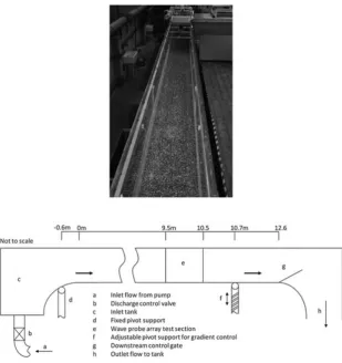
[7] A series of experiments was conducted in which the behavior of the water surface was altered by adjusting the general flow conditions of a range of steady, uniform shal-low flows over a rough, sediment boundary. During these tests, the dynamics of the free surface boundary were mea-sured carefully at a number of locations. The experiments were carried out in a 12 m long, sloping rectangular flume which is w = 459 mm wide (see Figure 1). The flume was tilted at a slope which varied from 0.001 to 0.004 in 0.001 increments. Volumetric flow rates of up to 0.03 m3/s were used in the reported experiments. The flume had a well-mixed gravel placed in its base and was scraped to a uniform level so there were no significant topographical features. The gravel particles had a density of2600kg/m3 and median grain size ofD50 = 4.4 mm. The measurement section was located at 9.5 m from the upstream end of the flume as shown in Figure 1. The bed surface roughness was measured at the test section of the flume using a laser dis-placement sensor attached to a computer controlled scanning frame. This was used to obtain elevation data of the sediment boundary on an orthogonal grid with a spatial resolution of 0.5 mm. The profiler was a Keyence LK-G82 laser displace-ment sensor. The bed elevation data were then used to calcu-late the second-order Kolmogorov structure function of the bed topography using the method proposed byNikora et al.
[1998] and extended to two-dimensional areas by Goring et al. [1999]. This method involves comparing a fixed section of the bed elevation data with a section of the same size whose position is translated within the scanned area. By assessing the correlation between the reference area and the translated area, a calculation can be made as to the corre-lation length of the bed topography in both streamwise and lateral directions. For this work, the reference and translated areas were 100 mm100 mm square. Figure 2 represents the bed structure correlation as the translated area is moved away from the reference area in the streamwise direction. This figure also shows the probability density function for the bed roughness estimated along the streamwise direction. It is apparent that above a lag of around 10 mm, there is no significant spatial correlation of the bed surface elevation. This suggests that any correlation observed on the water sur-face above this lag is not as a result of any feature on the bed having an individual influence on the flow surface, but that the surface pattern is generated by the bed roughness as a whole.
Figure 1. (top) A photograph of the hydraulic flume, and (bottom) sketch of the experimental setup in this flume showing the relative position of the measurement section with respect to upstream and downstream sections of the flume.
inlet pipe. The discharge was determined using a u-tube manometer connected to a standard orifice plate assembly [BS 5167-1, 1997]. The depth of the flow was controlled with an adjustable gate at the downstream end of the flume to ensure uniform flow conditions throughout as long a section as possible and in particular the measurement section of the flume. The uniform flow depth was measured with a point gauge and by means of wave probes.
2.2. Hydraulic Conditions
[9] The hydraulic conditions studied in this work were designed to investigate the change in the water surface pat-terns as a function of the flow depth and velocity for a range of submergences similar to those found in gravel bed rivers [e.g.,Ferguson, 2007;Robert, 1990]. For this study, 16 flow conditions were considered. A summary of the hydraulic conditions is given in Table 1. The uniform flow depth,D,
0 5 10 15 20 25 30 35 40
0 0.2 0.4 0.6 0.8 1 1.2 1.4
Streamwise displacement (mm)
−4 −3 −2 −1 0 1 2 3 4
0 0.005 0.01 0.015 0.02 0.025 0.03 0.035
Bed elevation (mm)
Structure function, 1 − W
(
Δ
)/
σ
2
[image:3.612.114.500.571.718.2]Table 1. The Characteristics of the Hydraulic Conditions Used for the Experiments
Bed Depth, Velocity, Equivalent Relative rms Elevation
Condition Slope D, (mm) V, (m/s) Re Roughness,ks, (mm) SubmergenceD/ks , (mm)
1 0.004 40 0.29 12000 19.0 2.10 0.34
2 0.004 50 0.35 19000 17.4 2.87 0.40
3 0.004 60 0.41 26000 15.1 3.97 0.45
4 0.004 70 0.45 32000 14.1 4.96 0.57
5 0.004 80 0.50 43000 13.3 6.03 0.74
6 0.004 90 0.53 52000 12.9 7.00 0.86
7 0.004 100 0.57 66000 11.8 8.46 0.97
8 0.003 50 0.26 14000 29.2 1.71 0.36
9 0.003 60 0.31 19000 24.3 2.47 0.43
10 0.003 70 0.35 26000 22.2 3.16 0.50
11 0.003 80 0.40 35000 18.3 4.36 0.58
12 0.003 90 0.45 43000 14.7 6.11 0.67
13 0.002 60 0.22 13000 39.7 1.51 0.23
14 0.002 70 0.25 18000 34.6 2.02 0.36
15 0.002 80 0.29 23000 26.3 3.04 0.43
16 0.001 70 0.17 12000 40.3 1.74 0.11
and the depth-averaged mean flow velocity,V, were varied from 40 to 100 mm and from 0.29 to 0.57 m/s, (Conditions 1 and 7, respectively). The equivalent roughness height,ks, for these conditions was calculated using the Colebrook-White equation modified for open channel flows [Barr, 1963]
1
p
f= –2.0 log10
ks 14.83Rh
+ 2.52 4Repf
, (1)
where
f=8gRhSf
V|V| (2)
is the Darcy-Weisbach friction factor,Sfis the energy slope,
gis the acceleration due to gravity,Rh =Dw/(2D+w)is the hydraulic radius andReis the depth-based Reynolds number. This number is calculated from discharge and mean water depth, which are each accurate to 0.5 l/s and 0.5 mm, respec-tively. The Reynolds number is calculated to two significant figures as shown in this table. The range of flow depths was produced so that the ratio of depth to equivalent roughness height (D/ks) varied from 1.51 to 8.46 (see Table 1), which is within the range of relative submergence values found in gravel bed rivers without appreciable bedforms byFerguson
[2007].
[10] For brevity, the shear velocity is not shown in Table 1, but it is used later in the manuscript for nondi-mensionalizing. The shear velocity can be easily calculated from the depth and bed slope data presented in Table 1 as U*=pgR
hSf.
2.3. Wave Probes
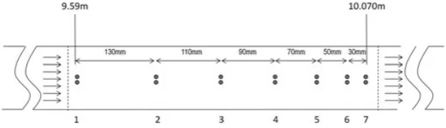
[11] A nonequidistant array of seven calibrated, conduc-tance wave probes was installed along the centerline of the flume at the test section to measure the instantaneous ele-vation of the water surface. Each of the probes in the array consisted of two vertical, parallel tinned copper wires which were separated by a 15 mm distance oriented laterally to the main flow direction. The diameter of these wires was 0.24 mm. The probe wires were attached to 2 mm thick plastic anchor plates which were held onto the base of the flume by the weight of the gravel layer. Since these anchor plates were below the gravel layer, they did not affect the flow. The top of each probe wire was attached to a screw mechanism allowing the wires to be held under tension to keep them vertical without exceeding the elastic limit of the wire and causing permanent deformation. Once the probes were calibrated, the tension was not altered. Figure 3 shows the position of the probe array with respect to the flume upstream end and indicates the streamwise separations between the individual probes. The wave probes were reg-ularly cleaned and calibrated to guarantee the accuracy of the water surface elevation measurements for the adopted range of hydraulic conditions. The calibration procedure involved recording the voltage levels for all the probes under static, still water conditions at six different water depths that spanned the full range of flow depths considered in this work (see Table 1). This allowed linear regression lines to be derived empirically to convert the instantaneous voltage recorded on a particular probe into an accurate instantaneous water depth.
[image:4.612.149.462.624.714.2]10−1 100 101 102
10−1 100 101 102
10−1 100 101 102
10−12
10−11 10−10 10−9
10−8
10−7
10−12
10−11
10−10 10−9
10−8
10−7 10−6
10−12 10−11
10−10 10−9
10−8
10−7 10−6
condition 1
0 5 10 15 20
−4 −3 −2 −1 0 1 2 3 4
x 10−3
x 10−3 condition 4
0 5 10 15 20
−4 −3 −2 −1 0 1 2 3 4
η
(mm)
Frequency (Hz) condition 7
0 5 10 15 20
−4 −3 −2 −1 0 1 2 3 4
Time (sec)
P
ower spectrum (m
2/Hz)
x 10−3
[image:5.612.100.516.57.566.2]10−6
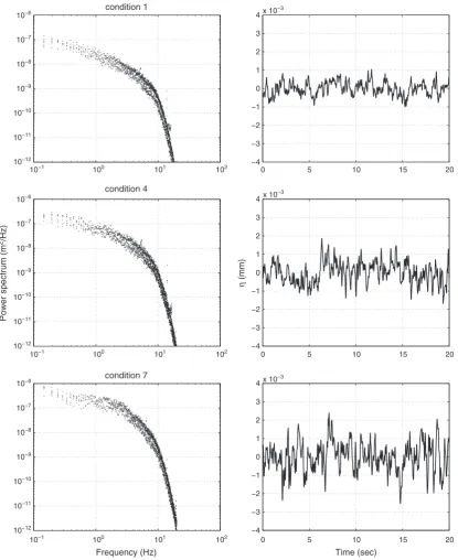
Figure 4. (left) The mean power spectrum of the water surface elevation for flow conditions 1, 4, and 7 and (right) example of time series recorded on probe 4.
[12] The probes were connected to standard WM1A wave probe control units provided by Churchill Controls. The out-puts of the probe control units were connected to a National Instruments X-series PXIe-6356 data acquisition card. The control units provided an analog output to the data acquisi-tion card, which was capable of measuring to an accuracy of 0.3 mV. This was over an input range of –10 to +10
V, which was tuned to cover depths from 0 to 200 mm, resulting in a measurement resolution of 0.003 mm. It was found that electrical noise was in the order of 1 mV or 0.01 mm, and for this reason, data presented in this manuscript are shown to two decimal places. The data acquisition card
digitized the analog wave probe signals simultaneously at 10 kHz in 1 millisecond packets. Each of these packets was acquired at a trigger rate of 100 Hz and the water level measured within each 1 millisecond packet was averaged to eliminate any chance of periodic high-frequency noise. The resultant 20 s 100 Hz digitized wave probe signals were detrended using a standard least mean squares technique. The 20 s duration for the recording of the wave probe sig-nals was sufficient to ensure that the standard deviation in the rms water surface elevation (see Table 1) settled to within
7 and the corresponding water surface elevation time series data recorded on probe 4. The data presented in Figure 4 are shown at frequencies below 20 Hz. The dominant spec-tral content is below 10 Hz, and the amplitude of the water surface elevation spectrum above this frequency is approxi-mately103times lower than the maximum amplitude. Also, the wave monitor itself includes a 20 Hz analog filter. This was also the cutoff frequency of a third-order low-pass Butterworth filter which was applied to remove high-frequency noise from the wave probe signals.
[13] As Figure 3 shows, some of the probes on which these signals were recorded were in close streamwise prox-imity to each other. This may give rise to the possibility of vortex shedding from an upstream probe generating capil-lary waves which would influence the data obtained from the downstream probes. The frequency of the flow structures which could potentially be generated by the vortex shedding was estimated using the Strouhal theory for two-dimensional flow over a circular cylinder [Posdziech and Grundmann, 2007]. For the range of velocities given in Table 1, the diameter-based Reynolds numbers for vortex shedding from a 0.25 mm-thick probe’s wire ranged from 80 to 170, giv-ing respective Strouhal numbers of 0.15 to 0.19 [Posdziech and Grundmann, 2007]. Vortex shedding at these Strouhal numbers and flow conditions would generate flow structures at frequencies of 200 to 500 Hz, which is well outside the range of the spectral components observed in the wave probe signals. Further, it can be shown empirically that the probe wires have a negligible impact on the statistical and spectral properties of the turbulence-generated surface roughness. In this experiment run at flow condition 5, individual probes were sequentially removed from the upstream end of the array so that only probe 7 remained in the array at the end. The signals from the probes in the progressively truncated probe array were recorded, and their statistical and spec-tral characteristics were compared against those obtained in the experiment with the original array. The first probe in the truncated probe array would provide a signal which had no interference from the remaining probes located down-stream. The other probes in this array would provide signals which could be potentially contaminated with the vortices shed from the remaining upstream probes.
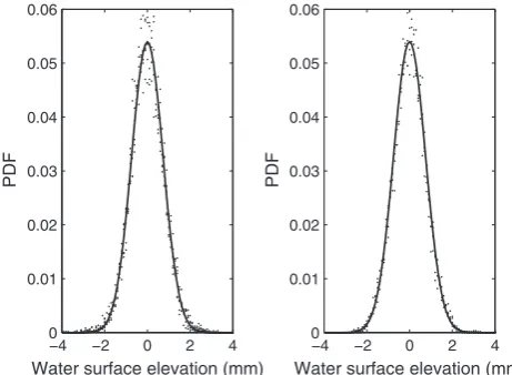
[14] Figure 5 presents the probability density functions calculated for the wave probe signals with and without potential interference in condition 5. The solid lines pre-sented in these two graphs correspond to the best fit for the Gaussian probability density function,p() = 1
p2e
2
22,
where is the water surface elevation. The values of the standard deviation (or rms water surface elevation) which correspond here to the best fit to the PDF data with and without potential interference are as follows: = 0.736
mm and = 0.749mm, respectively. These results show that the presence of the upstream wave probes results in lit-tle interference. More specifically, it is found that (i) the behavior of the probability density data for the water sur-face elevation measured using either a truncated wave probe array or the original, seven-probe array, closely follows the Gaussian distribution, a finding that is consistent with the quasi-Gaussian statistical behavior of the rough water flow surface reported in [Nazarenko et al., 2010]; (ii) the stan-dard deviation in the fitted Gaussian distribution changes
−4 −2 0 2 4
0 0.01 0.02 0.03 0.04 0.05 0.06
Water surface elevation (mm)
−4 −2 0 2 4
0 0.01 0.02 0.03 0.04 0.05 0.06
Water surface elevation (mm)
[image:6.612.312.543.59.228.2]Figure 5. The probability density function of the water sur-face elevation for flow condition 5 (left) with and (right) without probe interference.
only marginally (within˙2%) when an upstream probe(s) is removed; (iii) the scattering in the measured probability den-sity data for the wave surface elevation is relatively small, within the measurement error and it does not seem to change when the upstream probe(s) is removed; and (iv) the change in the PDF data related to removing one of the upstream wave probes is smaller than the degree of natural scattering in the signals recorded on the individual probes.
[15] Figure 6 presents the power spectral density, SQ(f), calculated for the wave probe signals whose probability den-sity functions are discussed in the previous paragraph (see also Figure 5). The solid lines in the graphs presented in Figure 6 correspond to the lines of best fit which were achieved using the functionlogSQ(f) = 1/(A+Bpf)with the following values of the coefficientsAandB:A = –0.0650
andB= 0.00518for the signal spectra with potential
inter-ference from the upstream probes; andA = –0.0644 and
B = 0.00506for the signal spectra without probe
interfer-ence. Here SQ stands for the power spectral density and f stands for the frequency in Hertz. The obtained spectral data also suggest that the effect of probe interference on the sig-nals recorded by the probe array is small and affects the measured power spectra by less than˙2%.
3. Free Surface Roughness in a Shallow
Water Flow
10−2 100 102
Frequency (Hz)
10−2 100 102
10−11
10−10
10−9
10−8 10−7
10−11
10−10 10−9 10−8
10−7
[image:7.612.64.296.56.230.2]Frequency (Hz)
Figure 6. The power spectra of the water surface elevation for flow condition 5 (left) with and (right) without poten-tial probe interference. The dots correspond to the individual wave probe data, and the solid curves correspond to the lines of best fit which is obtained using the functionlogSQ(f) =
1/(A+Bpf).
against the dispersion characteristics of the observed turbulence-generated water surface pattern. Gravity waves were generated in each case by impacting the free surface with a 50 mm square bar which had the same length as the flume width. This bar was applied perpendicular to the flow direction and parallel with the flow surface. In each case the bar penetrated the surface by 10 mm and then was quickly withdrawn to avoid the interference with the flow and with the resultant gravity wave. These experiments were designed to illustrate that in the presence of flow, the true velocity at which a gravity wave travels in the reference frame should also include the surface flow velocity component. There-fore, the gravity waves should propagate downstream faster than the mean surface flow velocity, whereas the turbulence-generated water surface roughness, which is unrelated to the gravity wave phenomenon, should propagate at a different velocity. If this is close to or less than the surface velocity then this suggests a link with underlying turbulent structures, as indicated byRoy et al.[2004].Guo and Shen[2010] sug-gested that propagating waves only account for 2.2 to 12.1% of the potential energy of the free surface, the rest being due to turbulence induced surface roughness.
3.1. Dispersion Relations for Gravity and Turbulence-Generated Waves
[17] Figures 8a and 8b show the time histories of the grav-ity waves recorded on wave probes 4–7 in the absence and presence of flow, respectively. Figure 8(c) shows the time history of the turbulence-generated waves in the flume under conditions similar to condition 4. The vertical scale in these graphs is the probe separation in meters. The amplitude of the wave probe signals here is not to scale. The top sig-nal in each of these two graphs corresponds to the upstream probe (probe 4 in Figure 3), and the graphs illustrate how the gravity wave propagates downstream from probe 4 to probe 7.
[18] The water surface elevation data for the gravity waves recorded on the wave probe array can be used to
calculate the phase velocity of these waves and compare it against that measured in the case of the turbulence-generated water surface roughness. The phase velocity of a wave,cp, is defined as the ratio of the wave frequency,!, to its wave number,k, i.e.,cp = !/k. In the case of a water wave, this velocity can be estimated using two different methods. The first method can be applied when there is a good degree of coherence between two water surface elevation signals,
m(t) andn(t), which are recorded simultaneously on two wave probes mand n separated by the distance mn. This can be the case, when a gravity wave with a reasonably deterministic shape propagates through a wave probe array. The phase velocity of this wave can be determined from the ratio of the Fourier spectra estimates form(t)andn(t). Provided that the attenuation of the wave between these two points is small, the phase velocity is given bycp(!) =
!mn
arg{On(!)/Om(!)}
, whereOm(!)andOn(!)are the Fourier spectra estimates of them(t)andn(t)signals, respectively. The second method can be applied when the behavior of the water surface elevation is more random, i.e., when the water surface roughness pattern caused by the turbulence in the flow appears as much more complex. In this case, the application of the above spectral method for phase veloc-ity estimation can be unsuccessful because the coherence between these two signals is likely to be too low to enable us to determine the phase difference,arg{On(!)/Om(!)}, with a sufficient degree of accuracy. In these circumstances, a bank of narrow band filters with center frequencies!jcan be adopted. The signalsm(t)andn(t)can be passed through this filter bank so that pairs of the filtered signalsm(t,!j), and n(t,!j) can be used to determine the lag at which the temporal cross-correlation function between these sig-nals exhibits an extremum,mn(!j). The phase velocity as a function of frequency can then be estimated fromcp(!j) =
mn/mn.
[19] The graphs shown in Figures 9 present the disper-sion curves for the phase velocity of the gravity waves in the presence and absence of flow and the phase veloc-ity of the water surface roughness observed for turbulent flow over the rough gravel boundary. The flow condi-tions in these experiments corresponded to those selected for condition 4 (see Table 1). Here the Fourier spectrum
[image:7.612.317.546.538.710.2]0 1 2 3 4 5 −20
0 20 40 60 80 100 120 140 160 180 200
Time (sec)
Probe separation (mm)
(a)
0 1 2 3 4 5
−20 0 20 40 60 80 100 120 140 160 180 200
Time (sec)
Probe separation (mm)
(b)
0 1 2 3 4 5
−20 0 20 40 60 80 100 120 140 160 180 200
Time (sec)
Probe separation (mm)
[image:8.612.129.482.56.366.2](c)
Figure 8. The time histories for the gravity waves and turbulence-generated waves measured in the flume under conditions similar to condition 4 (depth,D= 75 mm, the mean flow velocity,V= 0.49 m/s, and surface velocity,Vs = 0.7 m/s). (a) Gravity waves in the absence of flow; (b) gravity waves in the presence of flow; (c) turbulence-generated waves.
analysis method was used to determine the phase velocity of these gravity waves from the ratio of the phase spec-tra measured with two wave probes separated by a known distance. Correlation analysis (the second method which is described further in section 3.2) was applied to filtered flow data to determine the phase velocity spectrum with which the turbulence-generated water surface roughness pattern
appears to propagate. Figure 9a illustrates that in the absence of flow (still water), the phase velocity follows closely the theoretical curve which is obtained with the standard gravity wave theory found inLandau and Lifshitz[2000]. It is clear that in the presence of flow, the velocity of the gravity waves combines with surface flow velocity. The surface rough-ness patterns that we observe in the experiments detailed in
0 2 4 6 8 10
0 0.5 1 1.5 2
Frequency (Hz)
Phase velocity (m/s)
Still water (experiment) Still water (theory) Flow (experiment) Flow (theory)
(a)
0 2 4 6 8 10
0 0.5 1 1.5 2
Frequency (Hz)
Phase velocity (m/s)
(b)
[image:8.612.112.499.527.687.2]Table 2. Wave Probe Pairs and Spatial Lags Used to Calculate the Spatial Correlation Function of the Water Surface Roughness
Probe Pairs (mn) 77 67 56 45 57 34 23 46 12 47 35
Lag,mn(mm) 0 30 50 70 80 90 110 120 130 150 160
Probe Pairs (mn) 24 36 13 37 25 26 14 27 15 16 17
Lag,mn(mm) 200 210 240 240 270 320 330 350 400 450 480
section 2.2, however, propagate at a velocity that is close to that of the flow surface. Therefore, the water surface roughness patterns are not due to ordinary gravity waves.
[20] From this analysis it was found that the fre-quency dependence of the velocity at which the turbulence-generated flow structures propagate is markedly different to that measured in the case of the gravity waves (com-pare Figure 9a against Figure 9b). The velocity at which this pattern propagates is less than or equal to the flow sur-face velocity which is measured by timing the transport of a floating tracer over a defined length. This propagating veloc-ity is always between the mean flow velocveloc-ity and surface flow velocity (see Figure 9b) for all the experiments per-formed as a part of this study. These findings agree with the observations of [Smolentsev and Miraghaie, 2005] who also observed that water surface waves generated by strong tur-bulence appeared to have a celerity close to the mean flow velocity and that the celerity of gravity-capillary waves were different. These findings are also consistent with the parti-cle image velocimetry results reported byFujita et al.[2011] who suggested that the celerity of the roughness pattern on the free surface is lower but close to that of the surface veloc-ity. These observations clearly show a propagation velocity between the surface and depth-averaged velocity, suggest a link between the advecting surface features and underlying turbulent flow structures.
3.2. Correlation Characteristics of Turbulence-Generated Surface Roughness
[21] Under certain hydraulic conditions, the observed variations in the water surface elevations in a shallow water flow are controlled by the turbulent structures which emanate from the bed where the flow interacts with the fixed sediment boundary. These structures are transported and shaped by the flow and cause the distinct flow pattern which is clearly visible on the free surface (see Figure 7). The pat-tern of the water surface is continuously changing in time and space, and it is convenient to study its behavior in terms of the spatial correlation function which captures the sta-tistical and spectral characteristics of the dynamic water-air interface. The spatial correlation function is also a conve-nient measure of the coherence and variance in the water surface roughness between two points which are separated in space. In this way it is reasonable to suggest that the spatial correlation function can be used to estimate the amplitude of a coherent structure and speed with which it propagates and dissipates in the shallow water flow.
[22] The time-dependent signals measured with each probe pair in each of the flow conditions listed in Table 1 were cross-correlated to determine the maximum amplitude of the temporal correlation function (or its extremum). In this way the spatial correlation function for the water sur-face elevation above the uniform flow depth,W(,y,) = (x,y,t)(x–,y–y,t–)could be reconstructed for the values of that corresponded to the discrete spatial lags
between pairs of individual probes in the probe array, = mn. The number of unique probe pairs which can be used to calculate the spatial correlation as a function of the lag between the probes in a seven-probe array isN= 22which includes one extra point that corresponds to a probe corre-lated against itself (i.e., autocorrelation data for zero lag). Table 2 lists the probe pairs which were used to determine the values of the spatial correlation function and the dis-tances corresponding to the lag between each individual probe pair.
[23] In the reported experiments, the spatial correlation function was determined in two steps. Step I was to use data recorded on the seven-probe array to calculate the temporal, normalized cross-correlation function between probesmand nwhich is estimated from
–2W
mn(mn, 0,) = 1 T
Z T
0
m(t)n(t–)dt, (3) wherem(t)andn(t)are the time-dependent water surface elevations recorded on probesmandnwhich are separated by the distancemn,t is the time,T = 20sec is the mea-surement period andis the time lag. The root mean square (rms) water surface elevations,, are listed in Table 1. The value of for a given flow condition was determined as the average of the standard deviations for the data recorded on each of the probes in the wave probe array. The variation in the rms of the water surface elevations from one wave probe to another for a given flow condition was less that 10% which is supported with the probability density func-tion data shown in Figure 5. An observafunc-tion of the data listed in Table 1 suggests that the value of depends on the flow velocity and that generally increases with depth average flow velocity.
[24] The temporal, normalized cross-correlation function
Wmn() was then presented as a function of the distance
−0.1 0 0.1 −0.6
−0.4 −0.2 0 0.2 0.4 0.6 0.8 1
Condition 1
x (m)
Cross−correlation (−)
−0.1 0 0.1 −0.6
−0.4 −0.2 0 0.2 0.4 0.6 0.8 1
Condition 4
x (m)
−0.1 0 0.1 −0.6
−0.4 −0.2 0 0.2 0.4 0.6 0.8 1
Condition 7
[image:10.612.317.546.507.694.2]x (m) 0mm 30mm 50mm 70mm
Figure 10. The temporal cross-correlation data for flow conditions 1, 4, and 7.
can be explained by the complex interaction of flow struc-tures with multiple scales with the water surface, which is believed to be a pseudo-random process. The observed value of the correlation lag is controlled by the timescale of the production of coherent flow structures and by the advect-ing flow velocity that, in turn, controls how the observed water surface roughness propagates and dissipates. Since the coherent structures transported by the flow travel at (or near) the depth-averaged flow velocity [Roy et al., 2004], it seems reasonable that a spatial distribution of time averaged streamwise velocities over a rough boundary [Nikora et al., 2001] will result in a distribution of the advection velocities for the coherent structures. This explains why the temporal location of the cross-correlation extrema occurs within a dis-tribution about the temporal location for which all structures traveling at the mean flow velocity would occur. This level of spatial variability in the streamwise velocity relates well with the variability observed in the temporal position of the extremum value.
[25] Figures 10 show that the temporal cross-correlation functions obtained for flow conditions 1 and 4 flip their sign as the spatial lag between the probes increases from 0 to 70 mm. In these two conditions the flow depth is relatively low. As a result, the scale of the turbulent structures generated in these types of flow is believed to be relatively small and the structures themselves resemble whirls with some spa-tial scale, temporal period and characteristic lifetime [Hof et al., 2006]. Because the water surface roughness, which is caused by the propagation of these structures, is quasi-periodic, the correlation function is expected to flip sign. This type of behavior is typical for a correlation function of a quasi-periodic roughness process. The value of the spatial correlation function for this type of process will be negative when two wave probes in the probe array are separated by a distance of1/4L0 < < 3/4L0, where L0 is the charac-teristic spatial period. Clearly, when the depth of the flow is relatively low, then the scale of the turbulent structures is relatively small, and the pattern of roughness is relatively fine. In this case, the probe lags at which the data are plot-ted in Figure 10 (condition 1), are larger than1/4L0, so that
the correlation function flips its sign at a certain value of the lag. As the flow depth increases (see Figure 10 for condition 4), the scale of the turbulent structures increases propor-tionally and falls in the range of 40 < 1/4L0 < 50 mm. In this case, the flow roughness pattern is relatively coarse and the correlation function does not flip its sign until the probe lag becomes greater than 50 mm. Finally, when the flow is sufficiently deep (condition 7), the scale of the tur-bulent structures is large in comparison with the probe lag, hence the maximum of the correlation function is positive and the temporal cross-correlation functions do not flip for the probe lags reported in this work (see Figure 10 for con-dition 7). As Figure 11 shows, with greater spatial probe lag the correlation extrema do flip sign even for the deeper flow depths.
[26] The temporal correlation functions were obtained for all seven wave probe pairs and for all 16 flow conditions. The experimentally determined values of the spatial corre-lation function,W(mn, 0,e), for conditions 1, 4, and 7 are presented in Figures 11. These figures also present the error bars which illustrate the variability in the temporal corre-lation function extrema obtained using a number of wave probe recordings for each of these three conditions. The errors presented in these figures were estimated as the maxi-mum difference between the results obtained from the three reproducibility experiments. These findings enable the fol-lowing three conclusions: (i) the surface wave pattern has a clear characteristic spatial period; (ii) the amplitude of the spatial correlation function attenuates progressively as a function of the spatial lag, ; and (iii) the shape of the spatial correlation function can be best approximated with a simple analytical expression which is a combination of a periodic function and an exponentially decaying term which contain information on the characteristic spatial period of the turbulence-generated waves and on the correlation radius in the water surface wave pattern, respectively.
[27] A simple analytical expression for the spatial cor-relation function which combines the properties of an
0 100 200 300 400 500
−1 0
1 Regime 1
0 100 200 300 400 500
−1 0 1
Regime 4
Correlation coefficient
0 100 200 300 400 500
−1 0 1
Regime 7
Spatial separation (mm)
Table 3. The Deduced Values of the Water Surface Roughness Correlation Radius, Characteristic Spatial Period and Characteristic Wave Number for the 16 Hydraulic Conditions
Correlation Characteristic Characteristic Condition Radius,w, (m) Wave Number,q0, (1/m) PeriodL0, (m)
1 0.16 56 0.11
2 0.17 42 0.15
3 0.19 38 0.17
4 0.25 31 0.20
5 0.28 26 0.24
6 0.30 23 0.27
7 0.30 21 0.30
8 0.17 52 0.12
9 0.22 40 0.16
10 0.23 39 0.16
11 0.23 33 0.19
12 0.27 28 0.22
13 0.16 64 0.10
14 0.19 50 0.13
15 0.22 43 0.15
16 0.13 85 0.07
exponentially decaying function and a periodic process can be proposed. A suitable form for this expression is
W() =e–
2
w2 cos (2/L0), (4)
whereis the spatial lag. The parameterswandL0 in (4) carry a clear physical sense. The parameterwrelates to the spatial radius of correlation (correlation length). The value ofL0relates to the characteristic period in the surface wave pattern. Alternatively, the spatial correlation function can be expressed in terms of the wave number,q0 = 2/L0, that is characteristic to this particular water surface pattern, i.e.,
W() =e–
2
2wcos (q0). (5)
The choice of the Gaussian correlation function (or squared exponential covariance) is not uncommon. The function is smooth, differentiable and used widely to represent a quasi-stochastic surface roughness [e.g.,Paciorek, 2003;Bass and Fuks, 1979].
[28] It is desirable to estimate the values of w and L0 which correspond to a particular hydraulic condition. In this work the Nelder-Mead (simplex) bounded optimization method [Nelder and Mead, 1965] was adopted to find those values ofwandL0which would provide the best fit to an experimentally determined spatial correlation function. In this optimization process the criterion was the minimum of the function.
F(x) = 22
X
j=1
ˇ
ˇW(j,x) –W(j)
ˇ
ˇ, (6)
wherex= {w,q0}was the design vector. The values of the correlation radius, characteristic wave number and spatial period recovered from the optimization analysis are listed in Table 3 for the 16 hydraulic conditions studied. Figure 11 illustrates the fit between the mean experimental data for W(mn)(marker) and the values ofW()predicted by approx-imation (5) (continuous lines) for the values ofw andq0 taken from Table 3 for conditions 1, 4, and 7.
3.3. The Influence of the Hydraulic Condition on the Observed Free Surface Roughness Characteristics
[29] It has been suggested by Brocchini and Peregrine [2001] that if the water surface pattern is not associated with gravity waves then the spatial correlation pattern is related to the underlying turbulence. It is now useful to examine the spatial correlation parameters listed in Table 3 as a function of the corresponding hydraulic parameters listed in Table 1 for the 16 experimental flow conditions. A simple examina-tion of the data in Table 1 shows that the root mean square of the water surface elevation depends almost linearly with the depth-averaged velocity and flow depth. This simple rela-tionship also indicates that there is likely to be a physical connection between the bulk flow parameters and the water surface pattern. From Table 3 it can be seen that the values of the characteristic period and the correlation radius generally increase with depth although this pattern is less clear. Given the range of slope, velocity, and depth combinations, it was possible to determine generalized nondimensional relation-ships between the surface wave pattern and the underlying flow. Figure 12 shows that the nondimensional characteristic period demonstrates a strong consistent nonlinear relation-ship with the ratio of depth-averaged flow velocity to shear velocity. This figure indicates that the spatial characteristic length generally carries information on the shape of the ver-tical velocity profile and the underlying bed roughness for a range of hydraulic conditions. Figure 13 shows that the correlation radius, which reflects the dissipation of the sur-face pattern, can be nondimensionalized with the equivalent hydraulic roughness and can be shown to be a linear function of the flow Reynolds number and so carries a clear physi-cal sense that the spatial organization of the water surface waves is related to the dissipation of energy by the turbulent flow. Although the main aim of this paper was to study and quantify the spatial correlation patterns of free surface waves in shallow rough flows, the data collected and the analyti-cal function used to describe the spatial correlation provide clear evidence of a link between the surface pattern and the underlying turbulence and character of the shearing flow. By comparing the length scale of the water surface waves
0 2 4 6 8 10 12
0 5 10 15 20 25 30
0 1 2 3 4 5 6 7 0
5 10 15 20 25 30
[image:12.612.62.298.59.241.2]VD/ν
Figure 13. The dependence of the normalized correlation radius against flow Reynolds number.
with the scaling of the underlying turbulent flow features summarized byRoy et al.[2004], by demonstrating that the celerity of the flow features is different from gravity waves, and by indicating the similarity with some observations in other studies such asSmolentsev and Miraghaie[2005] and
Savelsberg and Van de Water[2009], we observe that the water surface correlation pattern is strongly controlled by the underlying turbulent flow features. Our observations do conflict to some extent with those of Savelsberg and Van de Water[2009] who conceptualized the water surface pattern generation mechanisms as a series of randomly gen-erated capillary-gravity waves that travel in all directions but whose scale is inherited from the underlying turbulent flow. These divergent views can however fit with the concepts first proposed byBrocchini and Peregrine[2001] and the exper-imental observations of Smolentsev and Miraghaie [2005] who identified a wide potential range of different water sur-face behaviors in which the different generation mechanisms can coexist, but noted that under some conditions certain processes dominate. For the hydraulic conditions close to the free surface flows encountered in gravel bed rivers, we proposed that it is the underlying flow turbulence that is the dominant process producing the spatial water surface pat-tern. Because of this dominance, the detailed measurement of the spatial properties of the water surface offers the poten-tial to deduce the character of the underlying turbulence. The existence of a physical linkage between the flow sur-face and the underlying turbulence, at submergences similar to those in gravel bed rivers, offers the potential for flow measurement in the field simply by measuring the water surface behavior and then determining its spatial correla-tion pattern. This means that flow measurement may now become possible in situations such as eroding or aggrad-ing channel reaches in which the physical placement of flow measurement instruments in the flow is not possible due to practical constraints.
4. Conclusions
[30] This work has reported on the water surface behav-ior of shallow turbulent flows over a rough sediment surface.
The flow conditions were selected to reflect those found in natural gravel bed rivers. These conditions have been reproduced through controlled laboratory experiments in a hydraulic flume with a rough gravel deposit with several constant bed slopes, variable depth-averaged flow velocity (0.17V0.57m/s), flow depth (0.040 D0.100m) and relative submergence (1.51 D/ks 8.46). In these experiments a nonequidistant array of wave probes has been used to study in detail the pattern of water surface elevations in the turbulent flow over a rough sediment bed. The pre-sented results illustrate that the wave probes do not interfere and are capable of measuring accurately the spatiotempo-ral pattern of surface waves. The comparative experiments illustrate that, for this range of hydraulic conditions, the free surface roughness is not due to ordinary gravity waves. The surface pattern of this roughness can be described by a spa-tial correlation function that is closely approximated with
a simple analytical expressionW() = e–
2
2w2 cos(2L–1
0 ), where is the rms water surface elevation, wis the spa-tial correlation radius, and L0 is the characteristic spatial period. This analytical expression was found to be appli-cable over the range of experimental hydraulic conditions. The parameterswandL0can define objectively the surface wave pattern which develops in this type of flow. The values of these parameters have been found to vary systematically with bulk hydraulic parameters and so were considered to carry a clear physical sense. The value ofL0 describes the characteristic period in the wave pattern observed on the flow surface, and the value of w relates to the rate with which the coherent turbulent structures dissipate in the flow. These findings quantify a clear physical linkage between the spatial correlation pattern of the water surface and the prevailing flow conditions and so pave the way to the devel-opment of a new measurement technique for the hydraulic processes in shallow, turbulent flows. The new method is based on the observation of the pattern in the water surface waves from which the nature and scale of the hydraulic pro-cesses in an open channel flow can then be inferred. This may allow measurements of hydraulic conditions in such shallow turbulent flows, when the insertion of conventional flow measurement instrumentation may not be possible due to practical constraints.
[31] Acknowledgments. This project was supported by the Engineer-ing and Physical Sciences Research Council (UK), grant EP/G015341/1. The authors are grateful to the technicians, Anthony Darron and Nigel Smith, for their contribution to the development of the experimental facil-ities used in this project. The authors are grateful to the associate editor and the three reviewers for their suggestions which helped to enhance the quality of this manuscript.
References
Babakaiff, C. S., and E. J. Hickin (1996),Chapter 17 in Coherent Flow Structures in Open Channels, John Wiley, New York.
Barr, D. I. H. (1963),Tables for the Hydraulic Design of Pipes, Sewers and Channels, Hydraulic Research Station, Wallingford, UK.
Bass, F. G., and I. M. Fuks (1979),Wave Scattering from Statistically Rough Surfaces, International series in Natural Philosophy, Pergamon, Oxford. Brocchini, M., and D. H. Peregrine (2001), The dynamics of strong
turbulence at free surfaces part 1: Description, J. Fluid Mech.,449, 225–254.
Buffin-Belanger, T., A. G. Roy, and A. D. Kirkbride (2000), On large-scale flow structures in a gravel-bed river,Geomorphology,32(3), 417–435. Dinehart, R. L. (1999), Correlative velocity fluctuations over a gravel river
bed,Water Resour. Res.,35(2), 569–582.
Ferguson, R. I., A. D. Kirkbride, and R. G. Roy (1996),Coherent Flow Structures in Open Channels, John Wiley, Chichester.
Ferguson, R. I. (2007), Flow resistance equations for gravel bed and boulder-bed streams, Water Resour. Res., 43, W05427, doi:10.1029/ 2006WR005422.
Fujita, I., Y. Furutani, and T. Okanishi (2011), Advection features of water surface profile in turbulent open-channel flow with hemisphere roughness elements,Vis. Mech. Proc.,1(4), doi:10.1615/VisMechProc.v1.i3.70. Guo, X., and L. Shen (2010), Interaction of a deformable free surface
with statistically steady homogeneous turbulence,J. Fluid Mech.,658, 33–62.
Goring, D. G., V. I. Nikora, and I. K. McEwan (1999), Analysis of the texture of gravel-bed using 2-D structure functions,Proc. IAHR Symp. River, Coastal and Estuarine Morphodynamics,1, 75–84, Madrid, Spain. Grass, A. J., R. J. Stuart, and M. Mansour-Tehrani (1991), Vortical struc-tures and coherent motion in turbulent-flow over smooth and rough boundaries,Philos. T. R. Soc. Lond.,336(1640), 35–65.
Hof, B., J. Westerweel, T. M. Schneider, and B. Echhardt (2006), Finite lifetime of turbulence in shear flows,Nature,443, 59–62.
Jackson, R. G. (1976), Sedimentological and fluid-dynamic implications of turbulent bursting phenomenon in geophysical flows,J. Fluid Mech., 77(3), 531–560.
Kirkbride, A. D., and R. Ferguson (1995), Turbulent flow structure in a gravel-bed river: Markov chain analysis of the fluctuating velocity profile,Earth Surf. Processes Landforms,20(8), 721–733.
Konmori, S., Y. Murakami, and H. Ueda (1989), The relationship between surface renewal and bursting motions in an open channel flow,J. Fluid Mech.,203, 103–123.
Kostaschuk, R. A., and M. A. Church (1993), Macroturbulence generated by dunes: Fraser River, Canada,Sediment. Geol.,85(1-4), 25–37. Kumar, S., R. Gupta, and S. Banerjee (1998), An experimental investigation
of the characteristics of free-surface turbulence in channel flow,Phys. Fluids,10(2), 437–456.
Landau, L. D., and E. M. Lifshitz (2000),Fluid Mechanics, page 36, chapter 1, section 12, Reed Education and Professional Publishing Ltd., Oxford.
Liui, Z., R. J. Adrian, and T. Hanratty (2001), Large-scale models of turbulent channel flow: Transport and structure, J. Fluid Mech.,448, 53–80.
Nazarenko, S., S. Lukaschuk, S. McLelland, and P. Denissenko (2010), Statistics of surface gravity wave turbulence in the space and time domains,J. Fluid Mech.,642, 395–420.
Nelder, J. A., and R. Mead (1965), A simplex method for function mini-mization,Comput. J.,7, 308–313.
Nikora, V. I., D. Goring, I. McEwan, and G. Griffiths (2001), Spatially averaged open channel flow over rough bed,J. Hydraul. Eng.,127(2), 123–133.
Nikora, V. I., D. G. Goring, and B. J. F. Biggs (1998), On gravel-bed roughness characterisation,Water Resour. Res.,34(3), 517–527. Nimmo-Smith, W. A. M., S. A. Thorpe, and A. Graham (1999), Surface
effects of bottom-generated turbulence in a shallow tidal sea, Nature, 400(6741), 251–254.
Paciorek, C. (2003), Nonstationary Gaussian processes for regression and spatial modelling, PhD Thesis, Carnegie Mellon University, Pittsburgh.
Posdziech, O., and R. Grundmann (2007), A systematic approach to the numerical calculation of fundamental quantities of the two-dimensional flow over a circular cylinder,J. Fluids Struct.,23(3), 479–499. Rashidi, M., G. Hetsroni, and S. Bannerjee (1992), Wave-turbulence
inter-action in free surface channel flows,Phys. Fluids A,4, 2727–2738. Robert, A. (1990), Boundary roughness in coarse-grained channels,Prog.
Phys. Geogr.,14, 42–70.
Roy, A. G., P. M. Biron, T. Buffin-Belanger, and M. Levasseur (1999), Combined visual and quantitative techniques in the study of natural turbulent flows,Water Resour. Res.,35(3), 871–877.
Roy, A. G., T. Buffin-Belanger, H. Lamarre, and A. Kirkbride (2004), Size, shape and dynamics of large scale turbulent flow structures in a gravel bed river,J. Fluid Mech.,500, 1–27.
Savelsberg, R., and W. Van de Water (2009), Experiments on free surface turbulence,J. Fluid Mech.,619, 95–125.