Advection on Graphs
The Harvard community has made this
article openly available. Please share how
this access benefits you. Your story matters
Citable link
http://nrs.harvard.edu/urn-3:HUL.InstRepos:38779537
Terms of Use
This article was downloaded from Harvard University’s DASH
repository, and is made available under the terms and conditions
applicable to Other Posted Material, as set forth at
http://
0.1
Overview
Advection on graphs is a natural translation of continuous advection, a partial differential equation that
describes the propogation of mass in a vector field, to continuous time and discrete space. The
continuous-to-discrete transition is implemented by assigning time-dependent real-valued masses to the graph’s vertices,
and orienting (and weighting) the edges on the graph to serve as the flow field. As far as I am aware,
it has primarily been given attention by Chapman [1], who approach the subject from the perspective
of coordinated control of multi-agent systems. (They mention a few independent employments of a similar
construction in the context of specific models of disease spread [2], population migration [3], and input-output
models in economics [4]). It is also briefly discussed by Grady and Polimeni in their Discrete Calculus[5].
The construction of advection on graphs is a first-order linear system ˙u= −Ladvu, whose matrix Ladv is
a modified version of the standard graph Laplacian. It has asymptotic long-term behavior, and can be
interpreted as the process of diffusion on a flow field.
Chapman [1] introduces advection as a modification of consensus, a system for cooperative control that has
been well developed in the past twenty years (see [6],[7],[8]). Consensus is very similar to diffusion on a
directed graph in that each connected component will obtain constant equilibrium values across nodes. In
contrast, advection has limiting behavior that is not constant across nodes within connected components.
As Chapman emphasizes, advection on graphs conserves mass. Unmentioned by Chapman but mentioned
by Grady et al. when they relate advection to PageRank, this conservation property actually hints at a
connection we will spend some time articulating: the relation between advection on graphs and Markov
chain theory.
First, we will give some background on undirected graph diffusion (the heat equation) and the matrix
differential operators connected to it. Next, we will introduce advection and observe a few preliminary
properties. Third, we will articulate the relationship between the solution to advection and the stationary
distribution of a Markov chain, and give an overview of relevant concepts from Markov chain theory. We
then tap on Markov chain theory to describe the categories and structure of advection’s limiting behavior, as
well as transient behavior. In so doing, we translate the applications of Perron-Frobenius theory developed
in the body of work on consensus to the advection setup. Last, we will introduce a some topological graph
0.2
Graphs and the Graph Heat Equation
We will work with directed graphs.
Definition 0.2.0.1. A graph G = (V, E) will be a set of vertices (nodes) V = {1,2, . . . , n}, and a set of
edgesE={e1, e2, . . . , em}, where each edge is named by an ordered pair of edges (i→j). 1
Definition 0.2.0.2. We define an orientation functionωwhose input is a nodeaand an edgee= (i, j) and
whose output is an integer as follows
ω(a,(i, j)) :=
1 ifa=j
−1 ifa=i
0 otherwise
Before we introduce the setup of advection, there are some objects in the discrete calculus on graphs setup
that are useful to be acquainted with.
0.2.1
Gradient Operator
If we consider a function on the graph vertices, u: V → Rn, how would we describe the gradient of this
function? We’d want the gradient of u to return information about the change in u with respect to the
degrees of freedom, which are the edges. The gradient operator will be a m×n matrix, where m is the
number of edges andnis the number of vertices. It is a map that takesuto its gradient;D:u→ ∇u. The
output of performing the gradient operator onuwill be a vector where each element corresponds to an edge.
2
Definition 0.2.1.1. On an oriented graphG we define thegradient operatorD asDi,j =ω(j, ei).
Consider as an example the graph below and its matrixD.
1We avoid usingvto refer to vertices since we’re saving the letter to denote the velocity field in advection.
2What’s different about the gradient operator of a graph is that it doesn’t return a vector for each “locality” it operates
Figure 1: Example graph. D=
−1 1 0 0 0
0 1 −1 0 0
0 0 1 −1 0
0 0 0 1 −1
−1 0 0 0 1
−1 0 1 0 0
0.2.2
Divergence operator.
The divergence operator is the transpose of the gradient operator. Intuitively, we want the divergence to tell
us for each vertex, the sum of the flow on the edges connecting to that node.
Definition 0.2.2.1. We define the divergence operator asDi,j:=ω(i, ej), and it isn×m, a map from the
edges to the nodes.
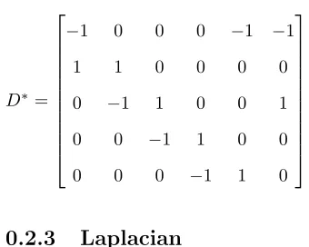
For the graph in 1 the divergence operator is
D∗=
−1 0 0 0 −1 −1
1 1 0 0 0 0
0 −1 1 0 0 1
0 0 −1 1 0 0
0 0 0 −1 1 0
0.2.3
Laplacian
Lij:=
X
k
D∗i,kDk,j
Fori=j we have (from above definitions)
Lii=
X
k
ω(i, ek)ω(i, ek)
=N(k), the number of edges connecting to nodek
Fori6=j we have
Lij=
X
k
ω(i, ek)ω(j, ek)
This is zero unlessiandj both share edge ek, in which caseω(i, ek) andω(j, ek) must have opposite signs,
meaning
Lij=
−1 if (i, j)∈E
N(i) ifi=j
0 otherwise
(1)
For the example graph above in 1, we have
L=
3 −1 −1 0 −1
−1 2 −1 0 0
−1 −1 3 −1 0
0 0 −1 2 −1
−1 0 0 −1 2
0.2.4
The Heat Equation
∂u ∂t =κLu
whereκis any constant, andLis the Laplacian defined directly above. This is an analogue of the continuous
heat equation, which has been transformed from an partial differential equation to a system of ordinary
differential equations.
We can solve it through the eigenvalue method: SinceLis symmetric, it has an orthonormal eigenbasis; we
can write the solution as a linear combination of eigenvectors:
∂u
∂t +κLu= 0 ∂
∂t X
i
biwi
+κL X
i
biwi
= 0
where the eigenvectors wi have unit norm, andbi, likeu, are functions of time
X
i
∂bi
∂twi+κ X
i
λibiwi= 0
X
i
∂bi
∂t +κλibi
wi= 0
∂bi
∂t =−κλibi
This means the solution u(t)
u(t) =X
i
bi(t)wi=
X
i
bi(0) exp (−κλit)wi
bi(0) is the initial condition u(0) projected onto the eigenvectorwi, ie
b(0) =
| | . . . |
w1 w2 . . . wn
| | . . . | u(0)
Ifλiis positive, the solution will decay to 0 along the corresponding eigenvectorwi. SinceLis positive
wi is in the kernel of L. The nullity ofL is in fact the space of functions on nodes where each connected
component has constant values throughout. This follows from the fact that the rows ofLsum to 0.
We could also circumvent the eigenvalues and eigenvectors via the matrix exponential method:
u(t) = exp[−κLt]u(0)
0.3
Introduction to Advection and Consensus
We introduce a discrete notion of advection by following the principle of flux from which the continuous
formulation is derived. In its original continuous formulation the advection equation is
du
dt =−∇ ·(¯vu)
where ∇· is the divergence operator, uis a conserved scalar quantity moving through ¯v, a time-invariant
velocity field on the domain of u. This formulation sets the change in mass at a point equal to the flux
through the point.
We start with a graph that has an orientation (i→j) defined on each edge. ¯vin the continuous case becomes
a vector inRm, the space of edges. We restrict the entries ofv to positive values, so that the flow is always
in the direction of the orientation of the edge.
We adopt the formulation of advection on graphs proposed by Chapman and Mesbahi. [1]. We’ll set up the
discrete analogue of the above formulation by requiring
dui
dt = X
(j→i)
ujv(j→i)−
X
(i→k)
uiv(i→k) (2)
ie, the change in mass at vertexiis the sum over edges terminating atiof the product of the velocity value
at the edge and the mass at the vertex from which the edge originates, minus the sum over edges originating
atiof the product of the velocity value at the edge and the mass at thei.
In matrix form we can rewrite 2 as:
The role ofDo, (o for originate) is to assign the masses at the verticesuto the edges originating at them.
It is defined as
Do(i, j) :=
−D(i, j) ifD(i, j)<0
0 forD(i, j)≥0
and as such is a modified gradient operator.
SinceD∗V Dois in fact a modified Laplacian, we can alternately say
du dt =D
∗V Dou=−L advu
where
Ladv=Dout(G)− Ain(G) (4)
is the advection Laplacian as defined in Chapman: The (i, i)th entry of the weighted diagonal matrixDout(G)
is defined asDi,i := P
(i→k)
v(i→k)∀i, that is, the sum of the weights of the edges going out of theith entry,
and the (i, j)th entry of the weighted adjacency matrixAin is defined asAi,j:=v(j→i), ie the weight of the
edge going fromj toi.
Here is the intuition for why 2 and 3 are equivalent: Moving right to left in 3, Douis a vector in edge space
where each entry is the value ofuat the vertex where that edge originates;V Douis the same with each edge
weighted by its velocity. When we apply D∗ and obtain D∗V Dou, we send to each vertex these weighted
entries on the edges connected to them, summed and given signs according to whether the edge is entering
or exiting the vertex. This is equivalent to the effect of 2, which for each vertex adds the vertex’s own value
weighted by its outgoing edges (Dout) to the negative of the vertices feeding into it (Ain). We mention the
formulation in 3 to illustrate the parallel to the standard Laplacian as the gradient of the divergence.
Ladv=
3 0 0 0 0
−1 0 −1 0 0
−1 0 1 −1 0
0 0 0 1 −1
−1 0 0 0 1
Now we effectively have a modification of the heat equation, still a first order linear differential equation,
where the Laplacian matrix is weighted, and is no longer symmetric.
Chapman and Mesbahi present advection as a modified verion of consensus dynamics, which are described
by
Lcons=Din(G)− Ain(G)
where (i, i)th entry of the weighted diagonal matrixDin(G) is defined as the sum of the weights of the edges
going into theith vertex, andAin(G) stays the same.
The consensus Laplacian for the previous graph is given by
Lcons=
0 0 0 0 0
−1 2 −1 0 0
−1 0 2 −1 0
0 0 0 1 −1
−1 0 0 0 1
As with the heat equation, the consensus Laplacian has a kernel of constant vectors, as is clear from the
example above. It does not, however, conserve mass as advection does, as we are about to show. First, we
note a useful relation betweenLcons andLadv:
Definition 0.3.0.1. [1] The reverse graph of G = (V, E, W) is the graph GT = (V, ET, WT) defined by
preserving the original vertex set, and creating a new reversely oriented weighted edge set (ET, WT) by
adding an edge (j, i)∈E with weightwij if there exists (i, j)∈E with weightwij.
Proposition 0.3.0.1. Ladv(G) = (Lcons(GT))T
It follows from the definition that Din(G) =Dout(GT). Since Lcons(GT) = Din(GT)− Ain(GT), and (b)
(Lcons(GT)T = (Din(GT)− Ain(GT))T
=Din(GT)−(Ain(GT))T
=Dout(G)− Ain(G) =Ladv(G)
An implication of this is thatLadv(G) and (Lcons(GT))Thave the same rank, which we will use in 0.5.2.1
0.3.1
Solution
Equilibrium Behavior
Since both the symmetric, unweighted L and the consensus Laplacian Lcons have a constant kernel, their
limiting behavior is to approach a constant, but the kernel of Ladv allows for more interesting limiting
behavior. How does the structure of a graph relate to the kernel of Ladv? This is the question we seek
to provide insight on. (We are able to directly compute the solutions, but we want to get insight beyond
this).
As we had before with the heat equation, our advection equation is a first order system of linear equations,
and has solutions of the form
u(t) =e−[Ladv]tu(0)
Unlike for diffusion,Ladvis not necessarily symmetric or diagonalizable. Still, solving advection is concerned
with the 0-eigenspace of Ladv, which we will demonstrate always exists. We will mostly be considering
contexts where the vector field we impose on the edges is identically valued for all edges—the case where V
is diagonal ones.
Positive semidefinite
Even though it is not symmetric, Ladv is positive semidefinite in the sense that for any vector w ∈
Cn, Re(w∗Ladvw)≥0. (We include complex numbers since as we will see,Ladv can have complex
w∗Ladvw=w∗(Dout− A∈)w
=w∗(D − A)w
=w∗Dw−w∗Aw
=
n
X
i=1
Di,i(wi)wi− n
X
i,j=1
(wi)wjAi,j
=1 2
Xn
i=1
Di,i(wi)wi−2 n
X
i,j=1
(wi)wjAi,j+ n
X
j=1
Dj,j(wj)wj
SinceDi,i= n P j=1 Ai,j =1 2 Xn i=1 ( n X j=1
Ai,j)(wi)wi−2 n
X
i,j=1
(wi)wjAi,j+ n X j=1 ( n X i=1
Ai,j)(wj)wj
=1 2
Xn
i,j=1
Ai,j|wi|2−2 n
X
i,j=1
(wi)wjAi,j+ n
X
i,j=1
Ai,j|wj|2
=1 2
Xn
i,j=1
Ai,j|wi|2− n
X
i,j=1
(wi)wjAi,j− n
X
i,j=1
(wj)wiAi,j+ n
X
i,j=1
Ai,j|wj|2
=1 2
Xn
i,j=1
Ai,j(wi−wj)(wi−wj)
w∗Lw=1 2
Xn
i,j=1
Ai,j(wi−wj)(wi−wj)
= 1 2
Xn
i,j=1
Ai,j|wi−wj|2
≥0
sinceAi,j is 0 or 1.
Since
Re(v∗Ladvv)≥0
Re(v∗λv)≥0
Re(λv∗v)≥0
Re(λ|v|2)≥0
Re(λ)|v|2≥0
Re(λ)≥0
all eigenvalues ofLadv have nonnegative real part.
Conservation of Mass
The advection system conserves mass [1]. To show this, we need to demonstrate thatP
i dui
dt = 0.
X
i
dui
dt = X
i
X
(j→i)
v(j→i)uj−
X
(i→k)
v(i→k)ui
= X
(j→i)∈E
v(j→i)uj−
X
(i→j∈E)
v(i→j)ui
= 0
This result is related to the result that we show in 0.4.1.
0.3.2
A Few Illustrations
Advection on a planar grid graph
Visualizing advection on a planar graph is a good starting example to demonstrate its properties and how
Figure 2: Advection on a grid graph with edges oriented north and east. A mass initialized in the southwest corner proprogates over to the northeast corner and stays there.
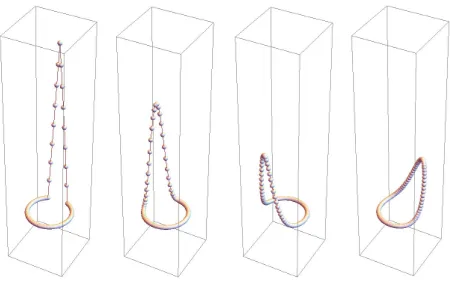
Advection on a cycle
ConsiderGR(n), a ring graph (aka circle graph, cycle graph) withnvertices andnedges. We will orient the
edges to point around the cycle (1→2,2→3, . . . , k→k+ 1, . . . , n→1).
With this setup the matrixLadv takes the form
Ladv=
1 0 0 · · · 0 0 −1
−1 1 0 · · · 0 0 0
0 −1 1 · · · 0 0 0
0 0 −1 · · · 0 0 0
..
. . .. ...
0 0 0 · · · 0 −1 1
Figure 3: Advection on a cycle graph with edges oriented counterclockwise. The mass propogates around the circle, spreading out as it does so, and eventually dies down to a constant.
As it turns out, simple and highly symmetric graphs such as the torus and the circle graphs obtain a constant
value in the equilibrium of advection. In fact, it follows from the definition ofLadv that any graph where all
vertices have the same number of ingoing and outgoing edges will obtain a constant in the equilibrium.
We seek to put together a language for describing the equilibrium values of advection for more complex and
asymmetric graphs.
0.4
Markov Chains and Perron-Frobenius
Characterizing the equilibrium behavior of advection on arbitrary graphs is done efficiently by recognizing
this object as a cousin of a Markov chain.
0.4.1
Relation between Advection and Markov Chains
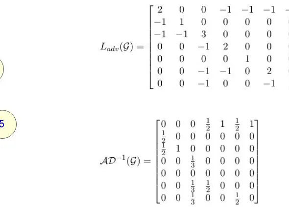
Recall our formulation of Ladv=Din(G)− Ain(G). The solution of advection is the solution of the system
LadvD−1y= 0 [5]
LadvD−1y= 0
(D − A)D−1y= 0
(DD−1− AD−1)y= 0
(I− AD−1)y= 0
(AD−1−I)y= 0
AD−1y=y
AD−1 is aleft stochastic matrix in that each column sums to 1:
RecallDi,i:= P
(i→k)
v(i→k), meaningDi,i−1:=
1
P
(i→k)
v(i→k)
andAi,j:=v(j→i), so
(AD−1)i,j=
v(j→i)
P
(j→k)
v(j→k)
and summing across rows:
X
i
(AD−1)i,j =
X
i
v(j→i)
P
(j→k)
v(j→k)
= 1
This means thatAD−1y=y can describe a Markov chain, as we will soon dive into.
If x∗ is the solution to the advection system Ladvx = 0 and y∗ is the solution to the Markov system
AD−1y=y, then we can obtainx∗ by solving the Markov chain and computing x∗=D−1y∗.
Figure 4: Advection/Markov chain connection example
0.4.2
Markov Chains
Definition 0.4.2.1. A finite state-space discrete Markov chain with initial distribution λ and transition
matrixP=pij (a stochastic matrix3 as defined in 0.4.1) is a finite sequence (X0, . . . , Xn) where
(1)X0 has distributionλ; ieP(X0=i0) =λi0
(2)P(Xn+1=in+1|X0=i0, . . . , Xn=in) =pin+1in.
This definition follows [11], pg. 2 with a few modifications (pin+1in instead of pinin+1 switchesP to being
left stochastic). I={i0, i1, i2, . . . , in}is the state space of the process and corresponds to the set of vertices
in a graph. We can think of a Markov chain as a object going on a random walk across the vertices of
a graph. (1) says that the vertex the object starts at is chosen according to some distribution λ (which
assigns a probability to each vertex). (2) says that once the starting vertex is chosen, the object proceeds to
navigate the vertex space according to probabilities assigned to the edges connecting to that vertex, which
is the entries{pji}.
3Note: we diverge from the standard convention used in statistics to express transition matrices asright stochastic and
It is then somewhat intuitive that this process should be connected to our notion of advection. As mentioned
in 0.4.1, the solution to the systemLadvx= 0 and the solution to the systemAD−1y =y (a Markov chain)
are related viax∗=D−1y∗, so the two are tightly related. We’ll discuss how the concepts of communicating
classes and expected visits, developed for Markov chain theory, translate to the advection system.
0.4.3
Communicating Classes
Definition 0.4.3.1 (Communicating Classes). For a Markov chain, stateileads to statej (or,i→j) if
P(Xn =j for somen ≥0|X0 =i)>0. If i→j and j →i, then the states i and j communicate and we
writei↔j([11], pg. 10, 11).
Sincei→jandj→kimpliesi→i, andi→i∀i, the relation↔imposes an equivalence relation on the set
of verticesI, and partitions the graphG. Each partitioned section—each set of vertices mutually reachable
to each other—is called acommunicating class.
Definition 0.4.3.2 (Irreducible). A Markov chain is said to beirreducible if all of its states are in a single
communicating class.
Definition 0.4.3.3 (Closed, recurrent, transient). A communicating class C is said to be closed if for a
given state i ∈ C, i → j =⇒ j ∈ C. A closed class is a communicating class that there’s no way
to leave. Intuitively, for a finite Markov chain, any state in a closed class is recurrent in the sense that
P(Xn=ifor infinitely manyn|X0=i) = 1.
On the other hand, if a state is called transient ifP(Xn =ifor infinitely manyn|X0 =i) = 0. This is a
state that it is possible to leave and never come back to.
Theorem 0.4.3.1. For any given communicating class C in a Markov chain, all states in C are either
recurrent or transient; that is, all communicating classes are either recurrent or transient.
Proof in Norris, [11], pg. 26.
0.4.4
Expected Visits and Stationary Distributions
Definition 0.4.4.1. A distributiony (a vector in vertex space) is said to beinvariantifP y=y.
Definition 0.4.4.2. Thehitting time(given by Tk) the first time (an integer) that the Markov chain visits
statek.
The expected number of visits to a vertexibetween visits to vertexk is
yk i :=Ek
Tk−1
P
n=0
1{Xn=i}=E
Tk−1
P
n=0
1{Xn=i}|X0=k
where 1Ais the indicator function of whetherAhappened.
Definition 0.4.4.3. A matrixAis said to bereducibleif there exists a permutation matrixP: PTAP is of
the form
X Y
0 Z
, whereX, Zare square, and 0 is a 0-matrix. A matrix that is not reducible isirreducible.
Theorem 0.4.4.1. ([11], pg. 35-36, modified)
If P is an irreducible matrix, then
yk= (yik:i∈I)satisfiesP yk=yk; ie it is an invariant distribution.
Proof
ykj =Ek Tk−1
X
n=1
1{Xn=j}
Because the state-space is finite, and because the irreducibility ofP ensures that every state will eventually
get to any other state (we prove this in 0.5.1.1), we can sayP(Tk<∞) = 1, or in other words
ykj =Ek ∞
X
n=1
1{Xn=j,n≤Tk}
Equivalently
=
∞
X
n=1
Rephrased by summing over all possible states previous toXn:
=X
i∈I ∞
X
n=1
Pk(Xn−1=i, Xn=j, n≤Tk)
=X
i∈I
Pk(Xn =j|Xn−1=i)
∞
X
n=1
Pk(Xn−1=i, n≤Tk)
=X
i∈I
pij ∞
X
n=1
Pk(Xn−1=i, n≤Tk)
=X
i∈I
pji ∞
X
m=0
Pk(Xm=i, m≤Tk−1)
We perform some reverse moves
=X
i∈I
pjiEk Tk−1
X
m=0
1{Xm=i}
ykj =
X
i∈I
pjiyki,so yk=P yk
This theorem gives us some insight into the nature of the stationary distribution: it is induced by the
effect of the graph connectivity on the expected visits to any given vertex. We will examine this further in
0.5.2.
0.4.5
Perron-Frobenius
Theorem 0.4.5.1. (Perron-Frobenius, [12], pg. 673 ) If An×n is an irreducible matrix, then the following
hold:
(1) Letσ(A)be the set of eigenvalues of A. Their maximum, r=ρ(A)∈σ(A), exists and satisfiesr >0.
(2) The algebraic multiplicity ofr is 1.
(3) There exists an eigenvectorx >0 :Ax=rx.
(4) The vector that satisfiesAp=rp, p >0,kpk1= 1 is called the Perron vector. There are no nonnegative
eigenvectors ofA except for positive multiples ofp, regardless of the eigenvalue.
0.5
Implications for Advection
To re-emphasize, the solutions to advection are easily computable; our goal in this section is to articulate
qualitative features of the solution to advection, building from the Markov chain theory and the theory on
the consensus. We’ll first establish some results relating the connectivity ofG to properties ofLadv.
0.5.1
Graph Connectivity
Definition 0.5.1.1. On a directed graph G, a globally reachable node is a node that can be reached from
any other vertex by a directed path.
Definition 0.5.1.2. On a directed graph G, a strongly connected component is a subgraph for which all
nodes are globally reachable. A graph that is entirely one strongly connected component is called strongly
connected.
A strongly connected component is equivalent to a communicating class.
Definition 0.5.1.3. A graph with at least one node that can reach every other node via a directed path we
will callweakly connected.
This is equivalent to the notion of rooted in-branching introduced in [1].
The concepts of irreducibility (as defined in 0.4.5) and strongly connected components are linked:
Theorem 0.5.1.1. For any strongly connected graph G,AD−1(G)is irreducible.([12]).
Proof. We’ll show that A(G) for a strongly connected graph is irreducible, which implies AD−1(G) is
irreducible.
Remark 0.5.1.1. If A is an adjacency matrix for some graph G, and P is a permutation matrix, then
B = PTAP is the adjacency matrix for the same graph G with its vertices relabeled according to the
permutationπgiven inP: PTAP isAwith its columns and rows rearranged according to the permutation.
This follows since Bij = 1 ⇐⇒ Aπ−1(i)π−1(j) = 1, meaning (i, j) is an edge in B’s graph precisely if
(π−1(i), π−1(j) is an edge in A’s graph, so (since π is a bijection)A’s graph andB’s graph are the same.
Having established this, we proceed.
By definition,Areducible means there is a permutation matrixP whereB=PTAP is of the form
X Y
0 Z
,
whereX, Z are square, and 0 is a 0-matrix. IfBisn×n, letX ber×randZ be (n−r)×(n−r). Ifαis
the set of vertices{1,2,3. . . , r} andβ is the set of vertices{r+ 1, . . . , n}, the bottom left 0-matrix means
that no vertex in αis connected to a vertex in β, so the graph with adjacency matrix B is not strongly
connected, and since it’s isomorphic to the graph with adjacency matrix A(by the above remark),G(A) is
not strongly connected.
(2) G(A) not strongly connected =⇒ A(G)reducible
IfG(A) is not strongly connected, then there is a way to label the vertices so that some subset of vertices
α={1,2,3. . . , r}has no connections to another set of verticesβ={r+ 1, . . . , n}. Then with respect to this
labeling we have an adjacency matrixB of the form
X Y
0 Z
, whereX, Z are square, and 0 is a 0-matrix.
LetP be the permutation matrix that gives a re-labeling of the vertices from whatever their original labeling
was to the labelling B uses. Then if Ais the adjacency matrix according to the original labeling, we have
B=PTAP, andAis reducible.
Lemma 0.5.1.1. If AD−1(G)is irreducible, rank(Ladv(G)) =rank(Lcons(G) =D − A) =n−1.
Proof. IfAD−1is irreducible, by 0.4.5 there exists an eigenvalueλ1=ρ(AD−1), with algebraic multiplicity
1. As a row stochastic matrix,ρ(AD−1) = 1 with algebraic multiplicity 1. This means dim(ker[I−AD−1]) =
1, and rank[I− AD−1] =n−1. [12]. And since (I− AD−1) =LD−1, rank(L) =n−1 as well.
Lemma 0.5.1.2. G has a globally reachable vertex if and only if rank(Lcons(G)) =n−1:
Proof in [13].
0.5.2
Graphs with Unique Equilibria
Most commonly studied in the context of consensus are cases where the Laplacian has a one-dimensional
kernel and solutions are unique. We comment on the properties of advection in this case.
Lemma 0.5.2.1. G is weakly connected if and only if rank(Ladv(G)) =n−1:
This follows from 0.5.1.2 and 0.3.0.1.
Definition 0.5.2.1. Let ansinkbe a strongly connected componentS for which no vertex inS has an edge
leading out ofS.
A sink is a subgraph whose vertices are contained within an closed recurrent communicating class.
Proposition 0.5.2.1. If G is weakly connected and has a proper subgraphS that is a sink, the basis of the
one-dimensional kernel of Ladv(G)will have nonzero values only at the vertices within the sink.
Proof. Begin with the sink subgraph alone and suppose it hasl vertices. Let the basis vector for the kernel
ofLadv(S) beuS = (u1u2. . . ul)T. By 0.5.2.2 we haveui>0∀i. By definition ∀i, l
P
j=1
Ladv(S)i,juj= 0. We
showed in 0.5.2.1 that the kernel ofLadv(G) must be one-dimensional. If αS is the set of vertices inS, and
αG is the set of vertices in G, by the definition of the sink there is no vertex inαS that has an edge leading
into a vertex inαG. This meansLadv(G) is of the form
Ladv(G) A
0 B
, whereBis (n−l)×(n−l) and 0 is
a 0-matrix. Then clearly if we addn−l 0’s to uS we will have a vector (u1u2. . . ul. . .0. . .0)T that is the
basis of ker(Ladv(G)).
So we’ve established that the dim(ker(Ladv)) = 1 situation occurs whenG is weakly connected, and that the
strongly connected subgraph, if it exists, will collect the mass. Within the strongly connected subgraph, the
cycle structure provides explanatory insight on the limiting solution, if we employ the results on expected
visits we covered in 0.4.4.
We’ll consider an example of how a small tweak to graph structure dramatically alters the solution form,
and demonstrate the connection to expected visits.
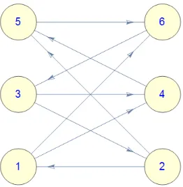
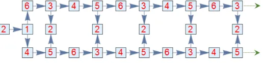
K3,3: A Demonstration of Cycle Effects
Consider the bipartite graph G =K3,3. The edges on G can be oriented such that half of them have two
outgoing edges and one incoming, and the other three vertices have two incoming edges and one outgoing
(a)G1: A “balanced” bipartite digraph. (b)G2: A bipartite digraph with a single edge reversed.
Figure 5: Two versions ofK3,3
In this case, if the edges are unweighted (all given weight 1), ker(Ladv) =c
1 2 1 2 1 2
T
—vertices
on the same side have the same value.
If we switch the orientation of a single edge (leaving all edges unweighted), it is still the case that three
nodes have two outgoing edges and one incoming, and three vice versa, but the equilibrium changes to
c
1 2 4 5 7 8
T
.
The theory developed for limiting distributions of irreducible Markov chains allows us to explain this
dif-ference in terms of the nodes’ recurrence times. Recall from 0.4.4 that for a Markov chain with transition
matrixP, the vectoryk that satisfies P yk =yk has its entries defined by
yk
i = the number of visits toibetween visits tok
(The choice of k does not change yk except up to a constant). And recall from 0.4.1 that the advection
solution is related to the Markov chain with transition matrixAD−1. When the edges are unweighted,AD−1
will be the transition matrix that assigns equal probabilities to each outgoing edge at a vertex.
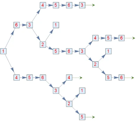
We can explicitly compute the entries of yk forG
1 by visualizing the possible walks that begin at vertex 2,
Figure 6: A walk diagram for G1
Consider the walks that begin and end at vertex 2. What is the expected number of times we hit vertex 3
across all these possible walks?
We can computey2
3, the expected visits to vertex 3 between visits to vertex 2 as
X
walks that hit vertex 3 once
P(walk)(1) + X
walks that hit vertex 3 2x
P(walk)(2) + X
walks that hit vertex 3 3x
P(walk)(3) +. . .
Upon examination, we can see that there are exactly 4 routes that begin and end at 2 and pass through
vertex 3 once. The first takes 2 forks, the second and third take 3 forks, and the fourth takes 4 forks,
so
X
walks that hit vertex 3 once
P(walk)(1) = (12)2(1) + (12)3(1) + (12)3(1) + (12)4(1)
Next, there are again exactly 4 routes that begin and end at 2 and pass through vertex 3 twice. The first
takes 4 forks, the second and third take 5 forks, and the fourth takes 6 forks, so
X
walks that hit vertex 3 2x
P(walk)(1) = (12)4(2) + (12)5(2) + (12)5(2) + (12)6(2)
y23= [(1 2)
2+ 2(1 2)
3+ (1 2)
4][1
· 1 22 + 2·
1 24 + 3·
1 26 +. . .]
= [1 + 1 2+
1 2+
1 4]
∞
X
n=1
n
22n
=9 4
4
9
y23= 1
By a symmetry argument, we can see thaty2
5= 1. Further, Figure 6 can convince us that every walk that
hits 3 a certain number of times before returning to 2, will hit 6 exactly the same number of times. The
same goes for 5 and 4. Last, the expected hits at 1 between visits to 2 is trivially 1, since any path leaving
2 must hit 1 first, and cannot reach 1 from any other vertex than 2.
We have established, then, thaty2=
1 1 1 1 1 1
T
. We said in 0.4.1 that ifx∗is the solution to the
advection system Ladvx= 0 and y∗ is the solution to the Markov system AD−1y =y, then we can obtain
x∗by solving the Markov chain and computingx∗=D−1y∗. Since (d
ii)−1= 1/2 for the odd vertices (since
they have 2 outgoing edges), and 1 for the even vertices, we obtain ker(Ladv) =c
1 2 1 2 1 2
T
as
desired.
Figure 7: A walk diagram for G2
We said we computed the advection solution to be ker(Ladv) =x∗=
1 2 4 5 7 8
T
. Soy∗=Dx∗=
2·1 2·2 2·4 1·5 1·7 1·8
T
=
2 4 8 5 7 8
T
(up to a normalizing constant).
Without getting into as much in-depth calculation as we did for G1, just by looking at Figure 7, it is clear
that every walk that hits 3 a certain number of times before returning to 1, will hit 6 exactly the same
number of times. And indeed, we have just computed thatyk
3 =yk6. Further, we can see that the walks that
hit 3ntimes before returning to 1 outnumber the walks that hit 2ntimes before returning to 1, by a factor
of 2:1. And indeed,yk
3 = 2y2k.
0.5.3
Rank of
L
advand Strongly Connected Components
Now that we’ve used Markov chain theory to provide some better intuition on the 1D solutions to advection,
we turn our attention to the multi-dimensional case.
Note that a graph can have overlapping weakly connected components. Note also that the number of sinks
can be less than the number of strongly connected components. Here is an example of a graph that has two
Figure 8: A graph with overlapping weakly connected components.
The subgraph with the vertices{1,2,3,4}is a weakly connected component that overlaps with the subgraph
with the vertices{2,3,4,5,6}, which is another weakly connected component.
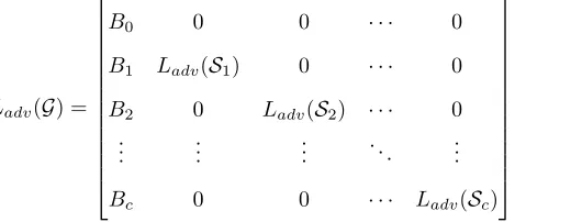
Theorem 0.5.3.1. If G has c sinksS1,S2, . . .Sk, . . . ,Sc, the rank ofLadv is equal ton−c, and the kernel
of Ladv is spanned by the vectorsuk= ker(Ladv(Sk)).
Proof. A graph with c sinks can have its nodes relabeled into groups α1 as the vertices ofS1, α2 as the
vertices ofS2, etc., andβ as the set of vertices ofGthat are in no sink, so thatLadv(G) is of the form
Ladv(G) =
B0 0 0 · · · 0
B1 Ladv(S1) 0 · · · 0
B2 0 Ladv(S2) · · · 0
..
. ... ... . .. ...
Bc 0 0 · · · Ladv(Sc)
whereB0is the portion of Ladv(G) that describes the interconnections between vertices in β, and Bk is the
portion of Ladv(G) that describes the interconnections between vertices in β and in Sk. Past B0, the top
row (of matrices) is 0 matrices because no node in one of the sinks has an edge leading out into a node
in β. (Recall the definition Ai,j :=v(j→i), the weight of the edge going from j to i). Further, all entries
above and below Ladv(Sk) are 0 since there is no node in one of the sinks that has an edge leading out
into a node in a different sink. Each submatrix Ladv(Sk) is of the same form as it would be as if it were
a standalone graph because the advection Laplacian is unchanged locally, since the diagonal only concerns
outgoing nodes.
(The trivial case is where the graph is entirely a single sink, which has a one-dimensional kernel as established
in 0.5.1.1.)
Since Lemma 0.5.1.1 established that each Ladv(Sk) individually has a kernel of dimension 1, then the w∗k
clearly span the kernel of Ladv(∪Si) =
Ladv(S2) · · · 0
..
. . .. ...
0 · · · Ladv(Sc)
. So any other vector in the kernel can
only have values that are not a linear combination ofw∗
k at vertices inβ. But this would mean, for somek,
that
B0 0
Bk Ladv(Sk)
has two (linearly independent) vectors in its kernel, and as the advection Laplacian
for a weakly connected graph, this violates 0.5.2.1.
0.5.4
Graphs with Multi-dimensional Limiting Behavior
In 0.5.2 we discussed the case where there is a unique limiting solution to the advection system Ladvx= 0
(the nullspace of Ladv is one dimensional), which results when G has a single sink. The result we just
established in the previous section allows us to address the remaining situations, which occur when G has
multiple sinks, and the limiting solution to the advection system is not unique.
We just established that the kernel of Ladv is spanned by the vectors w∗k = ker(Ladv(Sk)) (with zeros on
all nodes outsideSk). According to the general scheme we introduced for solving first order linear systems,
we can project our initial mass along the 0-eigenvectors, corresponding to the communicating classes, to
determine the final distribution of mass in advection. To rephrase what we discussed in 0.2.4, the solution
u(t) of a first order linear system is of the form
u(t) =P
i
bi(t)wi=P i
ci(0) exp (−λit)wi
wherebi(0) is the initial conditionu(0) projected onto the eigenvectorwi, i.e.
b(0) =
| | . . . |
w1 w2 . . . wn
| | . . . | u(0)
The solution will decay to 0 along all eigenvectors except those with 0-eigenvalues. If the c w∗
k span the
kernel, we have
u(t) =
c
P
k=1
bk(t)wk∗= c
P
k=1
bk(0) exp (−λit)wk∗
b(0) =
| | . . . |
w1 w2 . . . wc
| | . . . |
u(0)
In fact, if we replaced each sink with a single node, and computed the allocation of mass to that node, we
could then recursively solve advection on the sink as its own strongly connected graph using the techniques
from the previous section.
0.5.5
Random Graphs
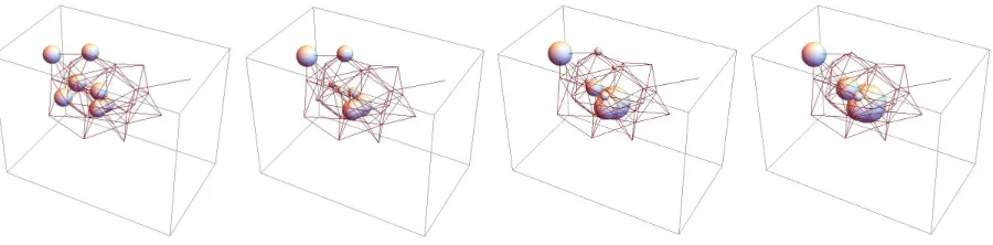
If we consider the behavior of advection on a randomly generated large graph (with randomly oriented
edges), it would make sense to expect there to be multiple sinks. Here is an example of the progression of
[image:29.612.85.535.316.427.2]advection on a randomly generated oriented graph with 35 nodes and 100 edges.
Figure 9: Advection on a random digraph with 35 nodes and 100 edges.
This graph has 5 single-node sinks, which accumulate the mass over time (and form a 5-dimensional kernel
forLadv). There is a good amount of room for potential future research exploring the statistics of patterns
of sinks in randomly generated graphs.
0.5.6
A Few Comments on Short Term Behavior
By now we have provided a fairly thorough treatment of the qualitative features of the long-term solutions
to advection. We’ll make a few short comments here on the spectral properties of Ladv that affect the
We established in 0.3.1 that all eigenvalues have positive real part, which is important since it confirms that
advection won’t explode. This is connected to a larger set of results on the spectra ofLcons:
Definition 0.5.6.1. The following properties are equivalent for a non-negative square matrix Atermed a
primitivematrix:
(1) there is aksuch that all entries ofAk are positive. [14]
(2)Aonly has one eigenvalue r=ρ(A) on its spectral circle ([12],pg. 674).
(3) The graph with adjacency matrixAhas the property that the set of all cycle lengths has common divisor
1. [6]
Matrices that are not primitive are called imprimitive, and a graph with an imprimitive adjacency matrix
has the property that the set of all cycle lengths has a common divisor k > 1 (the graph is called k
-periodic).[6]
Proposition 0.5.6.1. All eigenvalues ofLcons lie in a disk of radius 1 centered at the point1 + 0j in the
complex plane. IfA(G)is primitive, then all the nonzero eigenvalues ofLcons lie on the interior of this disk,
and if it is imprimitive, then its eigenvalues are distributed along the border of the disk. ([6])
The result in 0.3.0.1 connecting the consensus and advection Laplacian of graphs and reverse graphs,
Ladv(G) = (Lcons(GT))T, can be useful in translating these results on the spectra of Lcons to the
spec-tra ofLadv. For now we will stay content with the result on positive semidefinite-ness, and note one more
simple property:
Proposition 0.5.6.2. If a graphG has no cycles in it,Ladv(G)has entirely real eigenvalues.
This is because the nodes can be labelled such that Ladv(G) is lower triangular, and its diagonal entries are
positive real numbers, so the eigenvalues are all real. We can see this in the lack of oscillatory behavior in
the grid graph example in Figure 2.
0.6
Covering Graphs
The theory of covering graphs discussed in Gross and Tucker [15] and Sunada [16] has some interesting
implications on advection on a graph: given a covering graph and a base graph, the vertices in the fiber{ak}
in the covering graph have the same equilibrium values as the base graph had at its vertex a. 4 (Theorem
0.6.0.1).
First we’ll define a covering graph as according to Sunada:
LetG= (V, E) andG0= (V0, E0) be connected graphs.
Definition 0.6.0.1. [16] Amorphism from G to G0 is a set of a vertex map and an edge map f = (fV :
V →V0, fE:E→E0) that satisfies
ω(a,(i, j) =ω(fV(a), fE((i, j))
withωis as defined in 0.2, which is to say thatfV andfEpreserve the oriented adjacency relations between
the vertices.
A covering graph is a special type of morphism. Here is an example of a morphism that fails to be a covering
[image:31.612.171.437.310.432.2]projection, which we define next:
Figure 10: We can define a morphism from G, left, to G0, right, by sending a0, a1 →a;b0, b1→ b, c0 →c,
and (ai, bi)→(a, b),(bi, ci)→(b, c),(ai, ci)→(a, c). This satisfies the conditions of a morphism, but is not
a covering map.
Definition 0.6.0.2 (Covering map). [16] A morphism f : G → G0 is a covering map if it preserves local
adjacency relations between vertices and edges, that is, it satsifies:
(1)f :V →V0 is surjective.
(2) ∀a∈V the restrictionf|{e∈E:ω(a,e)6=0} :{e∈E:ω(a, e)6= 0} → {e∈E0:ω(f(a), f(e))6= 0} is a
bijec-tion. In other words, there is an orientation-preserving bijection between the edges attached to a vertex a
Here is an example of a covering projection.
Figure 11: We can define a covering map from G, left, to G0, right, by sending ai,→ a ∀a ∈ V(G0), and
(ai, bi)→(a, b) ∀(a, b)∈E(G0). This satisfies the conditions of a covering map. Example from Gross and
Tucker [15], pg. 59.
Proposition 0.6.0.1. If G coversG0 the size off−1(a)is the same across all a∈ G0:[16]
First, observe that for an edge (a, b)∈E0,|f−1((a, b))|=|f−1(a)|. This follows directly from the bijection
requirement in the definition of the covering map: If we pick a vertex a0 ∈ V : f(a0) = a, and there is a
local bijection between the edges Ea and f(Ea), then that particular a0 contributes one element to the set
f−1(a), and contributes one element to the setf−1((a, b)). Adding across all a0 we’ll get the same number
of elements in {f−1((a, b))} and{f−1(a)}.
It follows that for any edge (a, b), since|f−1(a)|=|f−1((a, b))|=|f−1(b)|, we have|f−1(a)|=|f−1(b)|. As
long as the graph is connected,|f−1(a)|must be the same for alla. If it is a finite numberk, thenf is said
to bek-fold.
We will now prove the following:
Theorem 0.6.0.1. For a graph G that covers a graph G0 via ak-fold mapf, let u∗0 = ker(Ladv(G0))and
u∗ = ker(Ladv(G)). For any vertex a ∈ V0, the entry of u∗ corresponding to any ai ∈ f−1(a) satisfies
u∗0(a) =ku∗(ai), where thek is independent of the choice of a.
An equivalent way of stating this is to say if we consider a covering graph as the state space of a Markov
specific fraction of the value ataof the stationary distribution of the covering graph).
This result means that covering graphs can be used as a tool for constructing distributed repeating
pat-terns of advection equilibrium on a graph. We can demonstrate this in the mobius strip graph
exam-ple (Figure 11). G0 in the example in Figure 11 is the same as the G2 in Figure 5, and has kernel
ker(LG0) = c
1 2 4 5 7 8
T
as we discussed in 0.5.2. Theorem 0.6.0.1 tells us that if we label
the vertices ofG accordingly, ker(LG) =c
1 2 4 5 7 8 1 2 4 5 7 8
T
.
Proof. Name the vertices of G0 a1, a2, . . ., and let vector functions u0 on the vertices of G0 be ordered
this way, and as well let the entries of Ladv(G0) (we’ll shorten this to LG0) be constructed with respect
that order. If k = |f−1(a)| is the fold of the covering map, and {an1, a2n, . . . , akn} = f−1(a1) is the
fiber of a1 we can choose to order the entries of a vector function u on the vertices of G according to
{a1
1, a21, a31, . . . , a1k, a12, a22, a32, . . . , ak2, a1n, a2n, a3n, . . . , akn, . . .}, and we can let the entries ofLG be constructed
with respect that order.
Letu∗0 ∈ker[LG0]. Expand u
∗
0 to a functionu∗ on the vertices ofG by repeating each entry ofu∗0 k times,
that is
a1 a2 · · · an ...
T
→
a1 a1 · · · a1 a2 a2 · · · a2 a3 · · · an−1 an an · · · an an+1 · · ·
T
We claimLGu∗= 0.
Consider thejth entry ofLGu∗. It is given by
LGu∗(j) =
X
i
LG(j, i)u∗(i)
= X
i∈V:LG(j,i)6=0
LG(j, i)u∗(i)
= X
i∈V:DG(j,i)6=0
DG(j, i)u∗(i)−
X
i∈V:AG(j,i)6=0
AG(j, i)u∗(i)
=DG(j, j)u∗(j)−
X
i∈V:AG(j,i)6=0
By the local bijection property of the covering map,
=DG0(f(j), f(j))u
∗(j)− X
i∈V:AG(j,i)6=0
AG0(f(j), f(i))u
∗(i)
By the construction ofu∗0,
=DG0(f(j), f(j))u
∗
0(f(j))−
X
i∈V:AG(j,i)6=0
AG0(f(j), f(i))u
∗
0(f(i))
=X
i
DG0(f(j), f(i))u
∗
0(f(i))
LGu∗(j) = 0
This result has an implication for expected visits as discussed in 0.4.4: if we start at some vertex b in a
covering graph G and make a sojourn back to b, the structure of G produces the result that the expected
number of times we hit someamin the fiber ofais precisely the expected number of times we hit any other
an in the same fiber.
This result also has potential implications for cooperative control. At the end of their paper, Chapman and
Mesbahi [1] discuss a few implementations of advection. In their first example, they connect a multi-agent
team via a cycle graph, and use the edge weights to control the geometry of the limiting configuration.
Specifically, since the graph is a cycle, the equilibrium value at a vertex is inversely proportional to the
weight of the edge projecting onto it. Were some application to arise where the connecting graph needed
to be unweighted or could not be weighted, the covering graph allows for the construction of a stereotyped
0.7
Conclusion
The goal of this report was to present advection on graphs as a mathematical object considered more
broadly and generally than simply as a construction for cooperative control as it was in [1]. While the
limiting solutions of advection are easily computable, viewing advection as a cousin of a Markov chain
provides further intuition and insight on the role of cycles in determining patterns in the solutions, as well
as on the character of solutions for graphs that are not irreducible, an area that has been largely sidestepped
by the cooperative control literature. Further, we hope to have sparked a possibly useful line of inquiry
into the employment of covering graphs for advection dynamics, and related constructions such as Markov
chains.
This report mostly focused on the limiting solutions of advection, but there is substantial room for further
work on characterizing the spectra of advection Laplacians, beginning with translating existing results on
the spectra of consensus Laplacians. In particular, there is certainly more to be worked out on the spectral
analysis of covering graphs. There is also a good amount of work to be done analyzing advection on
large random graphs: (a) in understanding how the sink structure of a graph depends on the probabilistic
parameters generating its oriented edges, and (b) characterizing the limiting behavior, as well as the spectra
Bibliography
[1] Airlie Chapman and Mehran Mesbahi. Advection on graphs. Proceedings of the IEEE Conference on
Decision and Control, pages 1461–1466, 2011.
[2] Mehran Mesbahi and Magnus Egerstedt. Graph theoretic methods in multiagent networks. Princeton
University Press, 2010.
[3] Roger A Horn and Charles R Johnson. Matrix analysis. Cambridge university press, 2012.
[4] Abraham Berman and Robert J Plemmons. Nonnegative matrices.The Mathematical Sciences, Classics
in Applied Mathematics, 9, 1979.
[5] Leo J Grady and Jonathan Polimeni. Discrete calculus: Applied analysis on graphs for computational
science. Springer Science & Business Media, 2010.
[6] J Alexander Fax and Richard M Murray. Information flow and cooperative control of vehicle formations.
IEEE transactions on automatic control, 49(9):1465–1476, 2004.
[7] Reza Olfati-Saber, J Alex Fax, and Richard M Murray. Consensus and cooperation in networked
multi-agent systems. Proceedings of the IEEE, 95(1):215–233, 2007.
[8] Reza Olfati-Saber and Richard M Murray. Consensus problems in networks of agents with switching
topology and time-delays. IEEE Transactions on automatic control, 49(9):1520–1533, 2004. [9] RB Bapat. The laplacian matrix of a graph. Mathematics Student-India, 65(1):214–223, 1996. [10] Ulrike Von Luxburg. A tutorial on spectral clustering. Statistics and computing, 17(4):395–416, 2007. [11] James R Norris. Markov chains. Cambridge university press, 1998.
[12] Carl D Meyer. Matrix analysis and applied linear algebra, volume 2. Siam, 2000.
[13] Francesco Bullo, Jorge Cortes, and Sonia Martinez. Distributed control of robotic networks: a
mathe-matical approach to motion coordination algorithms. Princeton University Press, 2009. [14] Shlomo Sternberg. Dynamical systems. Dover Publications, Inc., Mineola, NY, 2010.
[15] Jonathan L Gross and Thomas W Tucker. Topological graph theory. Courier Corporation, 1987. [16] T Sunada. Topological crystallography with a view towards discrete geometric analysis, surveys and