[NORMAL] When does a physical system compute?

White Rose Research Online URL for this paper:

http://eprints.whiterose.ac.uk/84119/

Version: Published Version

Article:

Horsman, Clare, Stepney, Susan orcid.org/0000-0003-3146-5401, Wagner, Rob C. et al. (1

more author) (2014) When does a physical system compute? Proceedings of the Royal

Society of London. Series A, Mathematical and Physical Sciences. p. 20140182. ISSN

1364-5021

https://doi.org/10.1098/rspa.2014.0182

[email protected]

https://eprints.whiterose.ac.uk/

Reuse

Items deposited in White Rose Research Online are protected by copyright, with all rights reserved unless

indicated otherwise. They may be downloaded and/or printed for private study, or other acts as permitted by

national copyright laws. The publisher or other rights holders may allow further reproduction and re-use of

the full text version. This is indicated by the licence information on the White Rose Research Online record

for the item.

Takedown

If you consider content in White Rose Research Online to be in breach of UK law, please notify us by

rspa.royalsocietypublishing.org

Research

Cite this article:Horsman C, Stepney S, Wagner RC, Kendon V. 2014 When does a physical system compute?Proc. R. Soc. A_470:

20140182.

http://dx.doi.org/10.1098/rspa.2014.0182

Received: 6 March 2014 Accepted: 11 June 2014

Subject Areas:

theory of computing

Keywords:

computation, physical computation, computer

Author for correspondence:

Clare Horsman

e-mail: [email protected]

When does a physical system

compute?

Clare Horsman

1

, Susan Stepney

2

, Rob C. Wagner

3

and Viv Kendon

3

1

_{Department of Computer Science, University of Oxford,}

Oxford OX1 3QD, UK

2

_{Department of Computer Science, and York Centre for Complex}

Systems Analysis, University of York, York YO10 5GH, UK

3

_{School of Physics and Astronomy, University of Leeds,}

Leeds LS2 9JT, UK

Computing is a high-level process of a physical system. Recent interest in non-standard computing

systems, including quantum and biological

computers, has brought this physical basis of computing to the forefront. There has been, however, no consensus on how to tell if a given physical system is acting as a computer or not; leading to confusion over novel computational devices, and even claims that every physical event is a computation. In this paper, we introduce a formal framework that can be used to determine whether a physical system is performing a computation. We demonstrate how the abstract computational level interacts with the physical device level, in comparison with the use of mathematical models in experimental science. This powerful formulation allows a precise description of experiments, technology, computation and simulation, giving our central conclusion:physical computing is the use of a physical system to predict the outcome of an abstract evolution. We give conditions for computing, illustrated using a range of non-standard computing scenarios. The framework also covers broader computing contexts, where there is no obvious human computer user. We introduce the notion of a ‘computational entity’, and its critical role in defining when computing is taking place in physical systems.

2

rspa.r

oy

alsociet

ypublishing

.or

g

P

roc

.

R

.S

oc

.

A

470

:2

01

40

18

2

...

1. Introduction

Information science is one of the great advances of the past century. The technology that developed from it is now integral to almost all aspects of day-to-day life in the developed world, and advances in mobile telephone hardware have put a computer in (almost) every pocket. In addition to the proliferation of semiconductor-based computers, non-standard (also known as unconventional) computational systems continue to be proposed and used—from the differential analysers of the early-twentieth century [1], through to the recent explosion of interest in quantum computing [2,3], and other proposals such as quantum annealing [4], DNA [5,6] or chemical [7,8] computational devices. The notion of computation, and its related system property, information, has been imported into other fields in an attempt to describe and explain such diverse processes as photosynthesis [9] and the conscious mind [10], and a strand of modern cross-discipline thought has given us the claims that ‘everything is information’ [11] or ‘the universe is a [quantum] computer’ [12].

In parallel with the technological and conceptual development of information science, its foundations continue to be addressed. The definition of which mathematical, logical and algorithmic structures constitute ‘a computation’ is a topic of ongoing research [13,14]. The question of how to define information, both as a concept and a physical quantity, is being investigated by philosophers, physicists and informatics researchers [15]. In this paper, we address a third, equally important, and specifically physical, question: what is a computer? Given some notion of a mathematical computation, what does it mean to say that some physical system is ‘running’ a computation? If we want to use computational notions in physics, then what are the necessary and sufficient conditions under which we can say that a particular physical system is carrying out a computation? In short,when does a physical system compute?

There is currently no accepted answer to this question, and an absence of a worked out formalism within which to determine whether a computation is happening physically gives rise to a great deal of confusion when discussing non-standard forms of computation. We can all agree that a laptop running a Matlab calculation and a server processing search engine queries are physical systems performing computation. However, when we move beyond standard and mass-produced technology, the question becomes more difficult to answer. Is a protein performing a compaction computation as it folds [16]? Does a photon (quantum) compute the shortest path through a leaf in photosynthesis [17]? Is the human mind a computer [18]? A dog catching a stick [19]? A stone sitting on the floor [20]? One answer is that they all are—that everything that physically exists is performing computation by virtue of its existence. Unfortunately, by thus defining the universe and everything in it as a computer, the notion of physical computation becomes empty. To state thateveryphysical process is a computation is simply to redefine what is meant by a ‘physical process’—there is, then, no non-trivial content to the assertion. A statement such as ‘everything is computation’ is either false, or it is trivial; either way, it is not useful in determining properties of physical systems in practice.

3

rspa.r

oy

alsociet

ypublishing

.or

g

P

roc

.

R

.S

oc

.

A

470

:2

01

40

18

2

...

abstract

(a) (b)

physical

e– _e–

abstract

physical

R ψ:iℏ— =∂_∂ψ Hψ

t ψ:iℏ— =Hψ

∂ψ

∂t

Figure 1.Representation in physics. (a_{) Spaces of abstract and physical objects (here, an electron and a wave function). (}b_{) The}

representation relation used as the modelling relationR_{mediating between the spaces.}

single, underlying structure. In all cases, we are dealing with questions of representation: how is a physical system represented mathematically, how do we test that representation and how can the representation be ‘reversed’, so that a physical system can instantiate a mathematical description. As well as computation, these are key issues in how we determine between scientific theories by argument and experiment, and in turn, fit into broader questions of representation that are fundamental to a number of different fields [21].

2. Physical computation

The question of when a physical system is computing is fundamentally a question about the relationship of abstract mathematical/logical entities to physical ones [22]. A ‘computation’ is a mathematical abstraction described in one of the logical formalisms developed by theoretical computer scientists. A ‘computer’ is a physical system with actual constituent parts and its own internal interactions that take it from one physical state to another. The computer is taken to stand in a certain relation to the computation—if we can formulate this relation, then we can answer our question of when a physical system is performing computation. To act as a computer is always to be performing a specific computation, we therefore need to ask: when isthisphysical system

performingthat(not always known) computation, and what is the relation required between the

physical system and the abstract computation that this can be determined?

The above gives us a view as infigure 1a: there is a space of abstract mathematical/logical entities and a space of physical entities. A computation is an entity in the first, and a putative computer in the second. So what is it that allows us to go between the two spaces? There is no possible notion of causation between them (this is simply a category error); so how does the abstract interact with the physical at all?

4

rspa.r

oy

alsociet

ypublishing

.or

g

P

roc

.

R

.S

oc

.

A

470

:2

01

40

18

2

...

3. Physics and the representation relation

The key to the interaction between abstract and physical entities in physics is via therepresentation relation[21,27]. This is the method by which physical systems are given abstract descriptions: an atom is represented as a wave function, a billiard ball as a point in phase space, a black hole as a metric tensor and so on. That this relation is possible is a prerequisite for physics: without a way of describing objects abstractly, we cannot do science. We have given examples of mathematical representation, but this is not necessary: it can be any abstract description of an object, logical, mathematical or linguistic. Which type of representation has an impact on what sort of physics is possible: if we have a linguistic representation of object weight that is simply ‘heavy’ or ‘light’, then we are able to do much less precise physics than if we use a numerical amount of newtons.

The most important property of the representation relation is that it is the relation that takes us across the divide between abstract and physical. The representation relation is unique in this respect, allowing a map between physical and abstract spaces: when we represent the physical and abstract as infigure 1(and subsequent figures), we are referring to the spaces themselves, not mathematical descriptions of them, and the representation relation is not a mathematical relation. Precisely, what it is, how it exists (and indeed can possibly exist) is a matter of ongoing research for philosophers of science; we know, nevertheless, that such a thing does exist. The representation relation is the relation that allows us to deal with the physical world at an abstract level; without it, any abstract reasoning about the physical world is not possible.

For a physicist, there is very little mystery in the representation relation: it is how physics

works. This relation is how we can write down |ψ and think that we are talking about an

electron or a hydrogen atom or a Bose–Einstein condensate. Every time we use something abstract to represent something physical, we use a representation relation. It is important to note that the representation of any given system is not unique: for example, a rubidium atom can be represented as a quantum bit (qubit), or as the solution to a master equation, or as a multi-level system with many orbitals.

This initial use of the representation relation in physics is fundamentally the process of

modelling: an electron is modelled as a wave function, an aeroplane as a vector and so on [21, part 1]. The modelling relationR_{takes an individual physical entitypto its abstract modelmp. We use} lower case for individual entities and uppercase for mappings between entities. Physical objects are given by bold letters, abstract by italics. We now have a picture as infigure 1b. This is the most basic use of representation, and we can immediately see that it is an asymmetric relation. Having an abstract representation for certain physical systems does not, in general, tell us how to find a physical system that matches a given abstract entity. When modelling, the physical system is known to exist (it is that which is modelled). However, there is noa priorireason to suppose that there is a physical system corresponding to every model. A theorist can write down, for example, the qubit state|ψ =α|0 +β|1; for an experimentalist, however, to discover and build a system to which it corresponds is often no trivial matter. While these two directions of representation are not absolutely disjoint, the exasperation sometimes expressed by experimentalists towards the unrealistic demands of theorists has its roots in the asymmetries of the representation relation between physical and abstract entities.

The two directions of the representation relation, modelling from physical to abstract, and instantiation from abstract to physical, lie at the heart of our questions around when a physical system computes. In physics, we represent the physical world using abstract and mathematical/logical concepts. In physical computation, we want to take an abstract entity, a computation and represent it physically. Put simply, abstract models may be created at will, whereas physical objects cannot. Without a simple relation that takes us from abstract to physical, how do we use the physical to instantiate the abstract?

5

rspa.r

oy

alsociet

ypublishing

.or

g

P

roc

.

R

.S

oc

.

A

470

:2

01

40

18

2

...

4. Theory and experiment in physics

The basic purpose of experiments in science is to test a modelling relation: is the model agood

model? At this stage of testing a theory, the only available representation relation is this modelling relation: we have a theory that takes us from physical to abstract, but not vice versa.

The models that are used in physics are not isolated, but rather located within specific, abstract, physical theories: an electron has a representation as a wave function in standard quantum mechanics, but as a point-mass in classical mechanics and as a vector in Fock space in quantum field theory. This is an important point: the representation relation is theory-dependent. When we test physical theories, we are testing, among other things, the representation that they give for physical objects. We therefore write the modelling relation asR_{T, where}T _{is the theory in which} it is located.

The model of a specific physical system, what we might call the kinematical representation, is then subjected to the dynamics of the abstract theory. For example, the wave function

ψ of an electron in a Stern–Gerlach apparatus would be described as interacting under a

given Hamiltonian dependent on the magnetic field strength. This can be worked out purely mathematically. Note that we are using the term ‘dynamics’ somewhat loosely; any theory of the physical system that produces output states from input states is applicable, whether it be couched in terms of evolution over time, or least-action principles, etc.

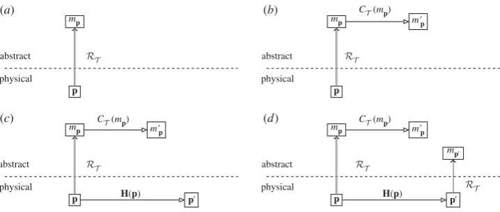
We now have the situation at the abstract level given infigure 2a: a physical systempis given an abstract representationmpby the modelling representation relationRT. This is then evolved

using the dynamics of theoryT_{,CT, resulting in the abstract systemm}′

p, as shown infigure 2b. Now, the physical systempis not, in general, static: it undergoes its own evolution in the physical world, H. The resultant physical system, after evolution, isp′, as shown infigure 2c. We now have the question about the relationship ofp′tom′

p. m′p is the abstract description, probably

mathematical, of how the theoryT _{thinks our physical system p should have evolved. How}

do we tell ifT _{has got it right or not? To do this, we need some way to comparep}′_withm′

p.

With only a modelling relation, we cannot construct a physical system fromm′p and compare

it withp′; however, we can construct a mathematical entity from p′, usingR_{T, and compare} it withm′p.

This gives us the situation infigure 2d: at the abstract level, we now have the abstractly evolved systemm′

p and the abstract representation of the physically evolved systemmp′. Two abstract

objects created by the same representation relationR_{T can now be directly compared.}

What we expect of a ‘good’ physical theory is that it produces a commuting diagram from figure 2d. In other words, the theoryT _{is such that we can either let a system undergo physical} evolution, or evolve it abstractly, and still reach the same place in the diagram corresponding to the ‘correct’ answer. This not a full specification of what it means to be a good physical theory,

but simply a minimal requirement: that the prediction of the theory,m′

p, is what we obtain in

reality. An absolutely commuting diagram therefore requires thatm′

p=mp′, and it would seem,

at first sight, that this is the requirement given in experimental physics: if the mathematical representation of the experiment outcome is not identical to the prediction, then the theory falls

under suspicion. Compare, for example, the diagram used by Ladyman et al. to define their

‘L-machine’ [28], which uses non-directional representation and requires absolute commutation. However, this is a much more stringent requirement than is used in practice. Experimental error and limitations of modelling mean that we are content ifm′p andmp′ are ‘close enough’: |m′

p−mp′|< ǫ. Exactly how big or smallǫcan be to be ‘good enough’ depends very much on the

context of the experiment: an undergraduate finding the energy levels of a well-studied SQuID for an assignment will probably impose a less strict closeness requirement than a team testing whether they have found the Higgs boson. The outcome in terms of the diagram, however, is the same: for the practical purposes to which it will be put, for the accuracy at which it has

been tested, the theoryT _{is such that the diagram commutes. Abstract predictions may then}

6

rspa.r

oy

alsociet

ypublishing

.or

g

P

roc

.

R

.S

oc

.

A

470

:2

01

40

18

2

...

abstract

(a) (b)

(c) (d)

physical

p p

m_p

m_p m_p

m_p m'_p

R_T abstract R_T

physical

CT(mp)

m'_p m'_p

m_p'

p' p'

p p

CT(mp) CT(mp)

abstract

physical

H(p) H(p)

abstract

physical

R_T R_T

R_T

Figure 2.Parallel evolution of theory and experiment. (a_{) Physical systempis represented abstractly bympusing the}

modelling representation relationR_{T of theory}T_{. (}b_{) Abstract dynamicsCT(mp)give the evolved abstract statem}′

p.

(c_{) Physical dynamicsH(p)give the inal physical statep}′_{. (}d₎R_{T is used again to representp}′_asmp′.

It is worth emphasizing again exactly what is involved in diagrams such asfigure 2, and

those for the Layman L-machine. These are diagrams indicating representation of physical objects (below the line) by abstract ones (above). Physical objects themselves are indicated below the line, not a mathematical representation of them. This contrasts with another set of diagrams that look at first sight very similar: those of abstract interpretation, where the concrete (operational) semantics for a computer is related to the abstract semantics for its programming [29]. While structurally similar to the diagrams here, abstract interpretation (as its name suggests) concerns entirely mathematical objects (the concrete and abstract semantics). The relations between them are straightforwardly mathematical relations. The representation relation, however, is not mathematical: therein lies the difference between the treatment of computers in theoretical computer science and our present concern to deal with them explicitly as objects in the physical world.

5. Commuting diagrams

We have spoken above somewhat loosely about a theoryT _{producing a commuting diagram for}

experiments. We now detail exactly whatT _{consists of, and its relationship to the representation}

and dynamics,R_{T andCT, used in our diagrams. First of all, though, we should note that we}

have not taken up a stance on what is needed for an experiment to confirm or refute a theory: all we are claiming is that any reasonable description of the scientific process must produce ade facto

commuting diagram.

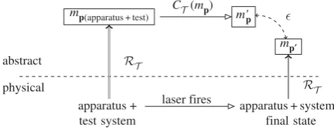
Let us consider an experiment to test a physical theory T_{test (figure 3). The physical set-up}

is denoted by p as before, and comprises the entire experiment. To take a specific example,

consider a rubidium atom in a cavity that is being excited by laser light in order to test a theory

of when its excited state will decay for a certain wavelength of incoming photons.pcomprises

both the atom that is being investigated and the apparatus (cavity, laser, detection devices, etc.):

p=p_test+p_apparatus. The apparatus is described by a theoryT_{apparatus. The abstract description}

of the experimental set-up,mp, is produced using the representation relation corresponding to the theory of the apparatus,R

T(apparatus).

7

rspa.r

oy

alsociet

ypublishing

.or

g

P

roc

.

R

.S

oc

.

A

470

:2

01

40

18

2

...

m_{p(apparatus + test)} m'_p

m_p¢

C_T(m_p)

abstract

physical

apparatus + test system

R T

apparatus + system final state laser fires

R_T

Figure 3.A ‘good enough’ commuting diagram for an experiment to test a theory. See text for details.

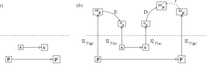
This combined theory,T_{, we can write as}T ₌T_test+T_{apparatus. The complete set of dynamics it} produces isCT. Applying these to the specific system modelmp to predict its evolution entails calculating the evolutionCT(mp). The result is the predictionm′p.

We now reach the final stage of the experiment. The entire experiment, apparatus plus atom, has evolved to its outcome state. In order to compare with the prediction, an abstract description of this final state is needed. This is produced by another use of the modelling relation for the apparatus, R_{T(apparatus). This is the step that takes us from, for example, current surges in a} detector to a description that a photon was detected at a certain time. We rely on our theory of the experimental apparatus to say that such an observed effect came from a photon, not any other kind of event. The fact that we must make use ofRT(apparatus)to represent the outcome of

experiments is known in the philosophy of science as thetheory-ladenness of observation[30]. There are no ‘basic’ observations that are unmediated by any kind of theory, all the way down to the level that when we see, hear or touch something we must form the theory that our senses are not deceiving us in order to correlate sense data with external objects.

Let us assume that the experiment was a success, and mp′ is close enough (by whatever

criteria we are using) to m′

p. The theory that then lives to fight another day is the combined

theoryT ₌T_test+T_{apparatusunder the particular circumstances of the experiment which used the} dynamicsCT(mp) of the combined systemp=ptest+papparatus. What has actually been tested in

this experiment is this very specific set of dynamics and representation: we have a commuting diagram forR_{T(apparatus)andCT(mp)—not}T _{itself. This is the reason why multiple experiments} on many different systems are considered necessary in order to argue for the correctness of a

theoryT _{(the process by which this actually happens being one of the foundational problems of}

the philosophy of science that we are not attempting to solve).

Moreover,T =T_test+T_{apparatus, and so if we want to use the experiment to test}T_{test, we need} to be sure aboutT_{apparatus. This means that}T_{apparatusmust previously itself have been subjected to} testing by a series of experiments, each of which formed their own commuting diagrams. These will be tests of both the dynamics and the model of the apparatus. If the theory of the apparatus, in either dynamics or modelling, is incorrect, then the experiment is flawed. An example of an

incorrect theory of apparatus was the 2011 announcement of faster-than-cneutrino speed by the

OPERA experiment [31]. A cable connected in an unexpected manner meant that the theory of the

apparatus was incorrect, and hence that the representationR

T(apparatus)to find the arrival time

measurement was flawed [32]. This gave an incorrect abstract descriptionmp′to the experimental

outcome (in that specific case, an incorrect time stamp to a detection event). As a consequence, an incorrect argument was made that the failure ofT ₌T_relativity+T_{apparatuswas owing to a failure}

ofT_{relativityrather than, as turned out to be the case, a failure of}T_apparatus.

8

rspa.r

oy

alsociet

ypublishing

.or

g

P

roc

.

R

.S

oc

.

A

470

:2

01

40

18

2

...

progression through progressively more ‘true’ theories. An experimentalist whose apparatus does not spring nasty behavioural surprises on them on a regular basis is fortunate indeed. We can therefore think of the whole process in terms of multiple interconnected diagrams, each of which is a specific experimental instance, for different theories (for example,T_apparatus+T_{test apparatus} to test the theory of the apparatus using another apparatus). Whatever the method turns out to be by which scientific theories are chosen (confirmation, refutation, explanatory power. . . ), the desired outcome is all these diagrams commuting. The scientific process can therefore be thought of as solving, by whatever method, this many-diagram satisfiability problem. The outcome of this process is then a set of theories that give rise to commuting diagrams in known cases, which we have confidence (however gained) will also produce commuting diagrams given other specific instances of a physical systempand its dynamics.

6. Reversing the modelling relation: prediction and technology

A theory producing a set of commuting diagrams is not the end of the scientific process. Once armed with a ‘good’ physical theory, it is then put to use (with the proviso, again, that we make no claim about the method by which theories are chosen as ‘good’). The theory itself can be seen as

an explanation of physical phenomena already known (the physical systemspthat were modelled

asmpand then used in the original experiments). The next step is to use the theory as apredictive tool, inferring the existence of phenomena, or even physical objects, about which we were previously ignorant.

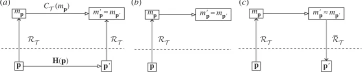
There are two stages to prediction in science. The first is the use of the modelling relation to give an abstract object that is then evolved. Based on a good theory, confidence that the complete

diagram,figure 4awould commute means that the physical evolution is not run: the abstract

evolution alone suffices to give the abstract representation of the physically evolved system. This is the ‘predict cycle’ (figure 4b): abstract evolution is used instead of physical to find the result

mp′≈m′

p.

If what is required out of a theory is an abstract prediction, then the cycle stops here. However, there is a second stage. The abstract theory has now been used to describe an abstract object different from the abstract descriptions of currently known physical objects. To what physical object does the abstract one correspond? Stated in terms of the modelling relation, this question becomes: what physical system, when modelled using our theory, will render this abstract object? In other words, we want to be able to reverse the modelling relation, to find a physical object corresponding to our new abstract description.

Reversing the modelling relation then requires us to have at our disposal an entire set of commuting diagrams, so that we can find the correct one to obtain a representation that in effect ‘runs in reverse’ from abstract to physical. This is a highly skilled and creative task for both theorists and experimentalists. There are many levels of interlocking diagrams that are involved in developing and testing a theory, and that are then produced when a theory is used to predict outside the range of physical events used to test it. While a reasonable level of confidence in a tested theory is needed in order to predict, prediction-and-instantiation diagrams,figure 4c, also become part of the many-diagram satisfiability problem that is the scientific process, as noted above.

Instances of prediction and subsequent discovery using scientific theories are, of course, numerous. One famous example is Dirac’s prediction of positrons [33]. By starting with a theory that had been experimentally tested using many physical systems, and using knowledge of the way in which the theory would model situations other that those that had been tested, the prediction was made that a particular abstract object in the theory (a hole in a sea of negative energy electrons) would correspond to a physical object (a positron). This prediction allowed a standard experimental cycle to be set up, and the diagram was found to commute.

9

rspa.r

oy

alsociet

ypublishing

.or

g

P

roc

.

R

.S

oc

.

A

470

:2

01

40

18

2

...

m_p m'_pª_m m_p m_p

p' m'pªmp' m'pªmp'

CT(mp)

p

(a) (b) (c)

p' p p

R

T RT RT RT R

~ T

H(p)

p'

Figure 4.Reversing the modelling relation within science: (a_{) a fully commuting diagram for physical and abstract evolution,}

based on a modelling relation only. (b_{) The ‘predict cycle’: abstract theory is used to predict physical evolution. (}c_{) The}

‘instantiation cycle’: using an instantiation representation relationR˜_{T, a physical object is found corresponding to the} predicted evolution.

but to construct them. This is the realm of technology: using our theories to precision-engineer physical systems to desired specifications. This is the final element needed in order, for us, to use this set of commuting diagrams as a framework in which to describe computation.

Engineering and technology are reversals of the modelling relation in a very specific manner. They start from the point of having a well-developed physical theoryT_{, which we have sufficient} confidence in to expect that it will produce diagrams that commute outside the situations in which it was tested. Within the representation of this theory, there is an abstract specification of the physical system that we wish to construct, which we will (leadingly) callmp′. The aim

of technology is to construct the corresponding physical system, p′, effectively reversing the modelling relation.

The process of technology to produce this reversal consists of finding a physical systemp,

the theoryT _{and a specific set of evolutionsHthat will perform the evolutionp}−→p′ such

that, whenp′is represented usingR_{T, it becomes the desiredmp}′. The physical systempis thus

engineered using the processHto produce the desired physical systemp′. An example would be taking a set of steel girders and building a bridge out of them.

A key consideration is how p, T _{and H are to be found. With a reliable theory, they can}

be discovered using abstract tools: in our bridge example, rather than physical trial and error

of different materials and construction techniques, a given starting point p can be modelled

abstractly asmp, then evolved to a final abstract statem′p. If this is close enough to the desired

mp′, then the correspondingpandHare good candidates for building the system. This is not a

mechanical or algorithmic process: the correctp,T _{andHcan be checked (at the very least, the} bridge can be built, and we can see if it falls down), but there is no straightforward process to select those for testing in the first place. This is an important fact about reversing the modelling relation: it requires ingenuity and skill on the part of the scientists and engineers involved. We can talk about a ‘reversed modelling relation’, or an ‘instantiation relation’, but only with the understanding that this is a shorthand for a whole sequence of preconditions. We write as a shorthand R˜_{T, understanding that} R˜_T ≡f(R_T,T_{) relies both on the theory} T _{that has been} developed, and on the primitive modelling relationR_{T. The equivalence is given infigure 5: the} physical systempevolves underHtop′which is represented inT _{as the desiredmp}′;T is such

that the representation ofpevolves abstractly tom′pandm′p≡mp′. The conjunction of these three

conditions is that the full diagram commutes. We can, then, reverse the modelling relation with

technology, but only when the theoryT _{is sufficiently advanced confidently to give commuting}

diagrams in all the cases we wish to consider.

7. When does a physical system compute?

10

rspa.r

oy

alsociet

ypublishing

.or

g

P

roc

.

R

.S

oc

.

A

470

:2

01

40

18

2

...

m_p m_p' m_p CT m'_p

p' p

p p

R

T RT

R~

T ∫

H

and and m'_pª_m

p'

Figure 5.Technology reversing the modelling relation:p,T_{andHare found such that these conditions hold. The combination} of these conditions is a commuting diagram.

relation{R_T,R˜_{T}and the dynamicsCT. We are sufficiently confident in our theory}T _{that we can} assume that it gives rise to commuting diagrams even when the exact starting states,pandmp, and the precise evolutions,CT(mp) andH(p), are different from the states and evolutions used in testing. Only when our physical theory of the computational device is sufficiently advanced that we can argue that all diagrams commute (in the scenarios, we will use it for) can the physical system be used as a computer. In this situation, as when the theory is used for prediction, we must have a sufficiently advanced and good theory that the representation relation can run in either direction.

The first distinction between computing and experimental science in this framework is the initial state. Previously, the physical statephas been the starting point; however, in a computation, the initial impetus is not a physical system that needs to be described, but rather an abstract object that we wish to evolve. An abstract problem is the reason why a physical computer is used.

We therefore start immediately with the problem of a reversed representation relation. The abstract initial state mp must be instantiated in a physical systemp: right from the beginning, we see that a computer is fundamentally an item of technology. Even to begin the process of computation, we require a well-understood and well-tested system. The reversal of the representation relation at the start of a computation is the process ofencodingabstract data in the physical system. It relies fundamentally on knowing exactly how the physical system works; on having a good enough physical theory to predict how data encodings will work. The encoding representation,R˜_{T, is not only dictated by the physics of the computer, but also by ourchoice}

of how to represent abstract computational objects such as numbers in physical systems. For

example, system designers in a standard semiconductor-based computer chosethe modelling

representation ‘voltage high→1, voltage low→0’. A crucial part of this choice is to make a

modelling relationR_{T that is easy to ‘reverse’ to obtain the}R˜_{T needed for encoding at the initial} stage of computation. Another example of anR_{T that is easy to ‘effectively reverse’ is the dial} input on a Babbage engine [34]. An initialpthat is the dial set to a certain angle is then represented as ‘0’, another angle as ‘1’, another as ‘2’ and so on. With appropriate markings on the dial, it is easy for the user to set up an initial physical situation that is represented as the desired number. In contrast, an example of a representation that is extremely difficult to ‘effectively reverse’ is given by the old-fashioned computers that used punch cards. A pattern of holes on a card determined the input (and indeed the program). Knowing exactly which holes to punch where (i.e. the exact physical statepto produce) such that it had the desired abstract representation (such as ‘01’) was considered extremely tedious and error-prone, requiring a great deal of skill and experience. In more recent times, anyone who has struggled to push the right buttons on their smartphone to do the simplest task has experienced a representation relation that was difficult to reverse, giving a difficult-to-use encoding relation. MakingR_{T sufficiently easy and intuitive to in-effect reverse} is a core component of designing and building a physical computing device.

11

rspa.r

oy

alsociet

ypublishing

.or

g

P

roc

.

R

.S

oc

.

A

470

:2

01

40

18

2

...

m_p mp

m_s 01, 10 CT (01, 10)

p'

p' p

(a) (b) (c)

p

p

R~

T

R~

T RT

R~

T RT

m_p'ª_m' p D

11 (gates)

H(p)

(voltage changes)

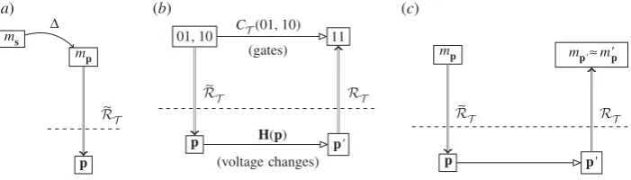
Figure 6.(a_{) Embedding an abstract problemmsinto an abstract machine descriptionmp using embedding}, then encoding intop. (b_{) Addition of two binary numbers using a computer (see text for details). (}c_{) The ‘compute cycle’: using}

a reversed representation relation to encode data, physical evolution of the computer is used to predict abstract evolution. Compare withigure 4c_.

using a calculator app. You embed this problem in the decimal division problem ‘50/6’, and then

encode this into the phone by pressing the correct buttons. The embedded problem,ms, is the

reason why we are interested in instantiating the specific set-up of the computational device that is abstractly represented asmp. For now, we will take the embedding as read and deal just with

mp; embedding will be discussed in more detail below, §8a.

With embedding and encoding relations in place, let us consider as a simple example a digital

computer running an algorithm that adds two 2-bit numbers, for example 01+10=11. We first

state how each of the individual pieces fit into the diagram offigure 2d, and then show how

computation proceeds.

The elements of the example are given infigure 6b. The abstract initial state, mp= {01, 10} is encoded, through the reversed representation relation (the encoding relation), in the physical systemp. This is the step ofinitialization:pis the initial state of the computer hardware (voltage across semiconductors, etc.). The representation relation has been derived from the theory we have about the physical components of device, of current and how it changes under voltage changes. Detecting a high voltage corresponds to representing a ‘1’, and low voltage is ‘0’. The initial physical set-up therefore instantiates an initial abstract state. In our example, two parts of

the hardware are designated byR_{T as ‘registers’, and the voltages in the components of those}

areas correspond to the representation of the initial state as ‘01’ and ‘10’ (the two numbers we wish to add).

At the abstract level, the initial state is used as the input to an algorithm: in this example, it is a sequence of gate operationsCT that takes the input ‘01, 10’ and adds them. An important part of

computation as actually used is that the result of the abstract evolution (here described in terms of gate operations) is not necessarily known prior to the computation. The final abstract state,

m′

p=(11), is not, in fact, evolved abstractly. Instead, at the physical level, a physical evolution

H(p) is applied to the state, producing the final physical statep′. In our example, this will be the hardware manipulation of voltages. Finally, an application ofR_{T takes the final physical state} and represents it abstractly as somemp′.

This final use of the representation relation is the decoding step: the physical state of the system is decoded as an abstract state. This is frequently simply the encoding step reversed, as in the above examples; however, it need not be. For example, NMR (classical) computing uses a heterogeneous representation. For a particular gate, the input bits are encoded as phases and time delays in the radio frequency pulses used to operate the gate, with different choices for each input ‘wire’; the output bit is decoded from the value of the observed integrated spectral intensity [35]. Note also that different decodings can give rise to different computations being performed overall even when everything else in the system stays the same [36].

After the final decoding step, if the computer has the correct answer, thenm′

p=(11). If we have confidence in the theory of the computer, then we are confident thatmp′=m′

12

rspa.r

oy

alsociet

ypublishing

.or

g

P

roc

.

R

.S

oc

.

A

470

:2

01

40

18

2

...

We can now see what it means to be performing a computation rather than to be an experiment. As we have seen, in experimental physics, a physical system is set up to parallel the abstract situation in order to test the abstract. The upper half of the diagram has been worked out in detail, and we run the lower half to compare with it. Once we have a commuting diagram, however, we no longer need to ‘run’ both halves: as long as the diagram commutes, and as long as our theory allows us to run the representation relation in both directions, we can proceed from initial state to final state by either abstract working or by physical evolution. Prediction and instantiation took us by an upper route from physical system to physical system via abstract prediction. Computation takes the lower route, starting in the abstract and ending in the abstract, via the physical computer.

This is physical computing: the use of a physical system to predict the outcome of an abstract evolution. The ‘compute cycle’,figure 6c, is an inverse of prediction and instantiation, in contrast to the latter’s use of abstract theory to predict the outcome of physical events.

We can now give the following as a set of necessary requirements for a physical system to be capable of being used as a computer.

— A theory T _{of the physical computational device that has been tested in relevant}

situations and about which we are confident.

— A representation{R_T,R˜_{T}of the physical system that is used for representing the initial} state of the physical system (encoding usingR˜_{T) and also for the final state, so that output}

is produced from the computation (decoding usingR_T).

— At least one fundamental physical computational operation that takes input states to output states.

— The theory, representation and fundamental operation(s) satisfy the relevant sequence of commuting diagrams.

All of these elements must be present in order for a physical system to be identified as acting as a computer.

8. Physical dynamics and computer programs

Up to now, we have considered the dynamics of the computer and the abstract computation as a single, indivisible evolution. We now look more closely at the structure of this evolution, as in general (and particularly in the case of universal computing), it is made up of smaller units. In a standard, digital, computer these are logic gates; other types of computation use units such as relaxation to a ground state (quantum annealing), or other dynamical operations (as in the case of the differential analyser). In the standard, gate-based, case the input is separate from the program, but in other cases, the initialization of the system can contain both the program and the input. In

that case, all the work is done by the representationR_{T, and the theoretical dynamicsC and}

physical evolutionHdo not change for different algorithms. The fundamental issues remain the

same in both cases and, for the sake of concreteness, we use the example here of a gate-based programmable computer. In this case, the first use ofR_{T determines initialization and the input;} Cis then the abstract program to be run, andHis the physical dynamics that will implement it.

We have referred to Chere as both ‘algorithm’ and ‘program’, and we now need to make

precise what we mean by this. An algorithm is a very high-level concept, detailing what is to be performed on an input, such as addition. However, in order to actually implement an algorithm, it needs to be broken down into components, and each of these components represented by fundamental operations—standardly, these are basic gate operations. This is the process of

refinementandcompilation. Once the basic operations have been determined for the algorithm, if there is a sequence of operations (as in standard gate-based computers), then they arecomposed

to be run on the physical computer.

13

rspa.r

oy

alsociet

ypublishing

.or

g

P

roc

.

R

.S

oc

.

A

470

:2

01

40

18

2

...

(a) (b) (c)

p(asm)

11

p'(asm) H(asm)

R~

T (asm) R

~

T (bin) R

~

T (dec) R

T (asm) RT (bin) RT (dec)

asm add

01, 10 01, 10

01, 10

11

R_BC

binary add

1, 2 3 1, 2

R_AB

R_BC

R_AB R_AB R_AB dec add

p(bin) H(bin) p'(bin) p(dec) p'(dec) 11

binary add

3

dec add

H(dec)

1, 2 3

dec add

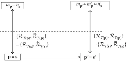
Figure 7.Physical computation, with layers of reinementR_{on top for base ten (decimal) addition (‘dec add’), binary addition}

(‘binary add’) and assembly language addition (‘asm add’). Note the physical device and representation difer in each case.

then the refinement and composition of the algorithm into machine descriptions that can then be encoded in the physical computer.

(a) Reinement

Refinement (or reification) is the computational process of taking an abstract algorithm, and producing a suitably equivalent concrete algorithm that is implementable on a computer [37]. The requirements for correct refinement (that the concrete design faithfully implements the abstract specification) also involve commuting diagrams; in this case, however, the diagrams live entirely

in the abstract realm. As an example, consider the algorithm for decimal addition. Figure 7a

shows the process of refinement from the abstract concept of mathematical base ten addition, through a more concrete concept of an algorithm for binary addition, to the most concrete (for this example) level of an assembly language program implementation of binary addition. Each level is in the mathematical realm, and can be proved correct with respect to the higher level. Some steps (usually the higher level ones) may require human design ingenuity; lower level steps can be performed automatically (computed) by an interpreter, compiler or assembler. Refinement of conventional computational algorithms stops in the mathematical realm, and assumes that the underlying physical device correctly implements the lowest level. Figure 7 shows the standard levels of refinement, positioned on top of our diagram for the underlying device: a physical assembly language computer. The relevant theory is that of the binary arithmetic. Accompanying theories that need to be developed are those of any relevant compilers and interpreters. Some of these accompanying theories can be purely mathematical (as they ‘implement’ formal refinement steps), but some of them have to cross the mathematical–physical divide.

For unconventional computational devices, where the lowest square commutes only ‘up toǫ’,

the traditional refinement approach of sequencing many computations would have to take error propagation into account.

The dividing line between the physical and mathematical realms is a design choice: more sophisticated physical devices can be engineered to perform appropriate refinement computations.Figure 7bshows the same abstract calculation, here refined only to the level of binary addition, and being implemented on a physical binary adder. Now, the relevant theory is that of the binary addition computer. This might be a combination of the theories of the assembly language computer and the relevant assembler.

14

rspa.r

oy

alsociet

ypublishing

.or

g

P

roc

.

R

.S

oc

.

A

470

:2

01

40

18

2

...

These diagrams all assume that the refinement described is possible. This need not be the case: there may be no possible embedding available, at one or more levels. This is the situation in which it is not possible to perform the desired computation on the given hardware. For example, there is no embedding that will allow an arbitrary billion digit integer to be represented in a machine with only a million bytes of memory: the machine simply is not large enough. The availability or otherwise of embedding steps tells us about the physical capabilities of our necessarily finite computers, as opposed to the arbitrarily large computations that can be described abstractly.

(b) Composition

The output of a refined and compiled process is a sequence of fundamental abstract operations that compose to produce the desired abstract process (the algorithm). Where a computation is composed of more than one fundamental operation, there are two parts to this: the fundamental operations themselves, and the rules by which they compose. For example, the set of operations could be AND, OR and NOT, and the composition rules will tell you, for example, what happens when an OR is followed by a NOT. We now look first at what it means to implement one of the fundamental operations in a physical system, and then at their composition where these are now all being run as physical computations.

A gate is an abstract evolutionCi. When applied to a particular (abstract) inputxit produces

the (abstract) output y=Ci(x). It is then the top line of a diagram of its own. To implement

this gate physically is to produce a physical system, a representation relation, and a dynamics of the physical system such that the resultant diagram commutes. To do this, the hardware designer uses exactly the same process of theory and experiment that we detailed above as experimental physics: the system is tested with multiple inputs, the representation and the dynamics scrutinized, and finally a theoryT_{iof the gate produced. This theory tells us that when} data are represented in such a way in the physical system then the dynamics produces such an output after the final representation. Confidence in this ‘gate theory’ means confidence that whenever the input is given in a specified way, the physical dynamicsHithat have been chosen

by this process of experimentation give rise to a commuting diagram.

Each individual gateCiis therefore tested, and the physical theory (which gives the encoding

and decoding) T_{i developed of the gate produces its own commuting diagram with a given}

physical system p_i, representation R_T

i and physical dynamicsHi. We also require, as well as

individual theories of gates, a theory T_{C that describes how they compose (making sure that}

they do not, for example, contradict each other). As with all physical theories, this compositional theory will be produced by the interaction of theory and experiment, and give rise to its own commuting diagrams with the physical system that is being used as a computer.

The theory of the physical computer is therefore developed in order to predict the outcome in situations that are unknown—exactly as we use theories in physics. This theory is then extended and tested further, in exactly the same way that any physical theory is developed. The end result of this testing and development is a computer, and the theory that governs it,T _{= {}T_C,T_i}. What confidence inT _{gives is confidence that, within the limits of}T_{, any diagram that can be} written (i.e. any input and any program), will commute. The physical system, the computer, can then with confidence be used to find the result of abstract evolutions written as compositions of the fundamental gates. When any (Turing) computable abstract evolution can be so written,

the computer is (Turing) universal[14, ch. 3]. A universal computer has the property that the

hard work of experimentally producing commuting diagrams need only be done once, then the computer can be used for any computation.

9. Computational entities

15

rspa.r

oy

alsociet

ypublishing

.or

g

P

roc

.

R

.S

oc

.

A

470

:2

01

40

18

2

...

relation is used to encode abstract data and programs in the physical system, and then at the end it is used to decode the state of the physical system into an abstract output. Without the encode and decode steps, there is no computation; there is simply a physical system undergoing evolution. This, then, is one of the key ways in which this frameworks distinguishes between a physical system ‘going about its business’, and the same physical system undergoing the same physical evolution, but this time being used to compute. This is how we can escape from falling into the trap of ‘everything is information’ or ‘the universe is a computer’: a

system may potentially be a computer, but without an encode and a decode step it is just a

physical system.

The question of whether a given physical system is acting as a computer then becomes a question of representation at two different levels. Can we represent what is going on, physically and abstractly, as including an encode and decode step, i.e. as including representation? A necessary condition of there being representation present is that there is, as well as the computer, an entity capable of establishing a representation relation. That is, an entity that represents

this specific physical system as this specific abstract object, encoding and decoding data into

it. Something must always be present that is capable of encoding and decoding: if there is a computer,whatis using it?

The necessary existence of a computational entity is a fundamental and integral part of the framework presented here. Without this requirement, there is no differentiation between computation and ordinary physical evolution. It also, at first sight, goes completely against the grain of objective science. Perhaps the most important conceptual breakthrough of information science at its inception was the separation of information as a quantity from its meaning [38]. The former could be discussed independent of any person or thing performing the computation, whereas the latter was irredeemably subjective. If we are now saying that computational processes cannot be described independently of computation entities (human or otherwise), then an immediate concern is that the act of computation then becomes wholly subjective, possibly subjected to the intent of the entity running the computer, and not something that can be dealt with by an objective scientific theory of computation. This is an important concern, which we now address.

The first thing to note is that all the requirements we have given, including the requirement that a computational entity responsible for representation be present, are objective requirements. It is simply an objective fact of the matter whether or not a computational entity is part of the system. Consider, for example, that you are watching a student work out a problem using a calculator. There is nothing subjective about the existence of the student. Furthermore, the requirements on the computational entity are not subjective (there is no requirement, for example, for an intent to compute or any subjective position to be taken up towards the computational device): the requirement is that an encoding and a decoding are present, an objective fact of the matter. By close observation of the student, you can determine whether information is being encoded into and decoded from the calculator. You as the observer can formulate and test the hypothesis that the student and calculator form a computing system. If you and another observer differ in your theories, there is a fact of the matter as to which of you is correct (although, as with any scientific theory, you may not have all the data required to settle the question). Fundamentally, the question of computational entities comes down to the question of the objective existence or otherwise of encoding and decoding. The entities are required only, because encoding/decoding cannot be defined otherwise, not because encoding/decoding is subjective or perspectival.

16

rspa.r

oy

alsociet

ypublishing

.or

g

P

roc

.

R

.S

oc

.

A

470

:2

01

40

18

2

...

device, the computational entity responsible for the representation relation between abstract and physical must be physically realized.

There is a very close and important relationship here with another branch of computational theory: communication theory, and how it uses the parties in a transmission to describe the transmission of information. Usually termed Alice and Bob, the communicating entities are responsible for encoding information into a signal at one end, and decoding it at the other. While a theoretical treatment of a communication scenario need deal only with the transmitted signals, actually sending a message requires Alice and Bob. We can, in fact, locate communication entirely within our framework for computing: the encode and decode steps remain (usually performed by distinct spatio-temporally separated entities), and the evolution of the physical system is an identity computation (the message remains the same between sender and receiver). The definitions of computational and communicating entities coincide.

As with a communicating entity, there is nothing in the definition of acomputationalentity

that requires it to be human. There is also no need to bring in ill-defined descriptions such as ‘conscious’ or not. Communication theorists refer as a matter of course to computer terminals, or circuits, or photodetectors as the communicating entities. Simply, anything that is capable of encoding and decoding information is a computational entity. Whether or not any given entity is capable of this is an objective fact of the matter about which hypotheses can be formulated, tested and argued over. Part of the objective description of the computational entity is the sophistication of the encoding and decoding operation that it is capable of supporting. If the computational entity is a human being, then we are fairly certain about what representations it is capable of. If, for example, a person were writing a computer program to solve a second-order differential equation, then we would happily describe the encoding and decoding operation as just that. If, on the other hand, a cat walked across the keyboard and randomly touched exactly the right keys to type out that same program, then it would not be a good hypothesis that it was calculating a differential equation. To argue that it was would require the cat to be capable of a complexity of encoding and decoding (including a knowledge of differential equations) that we usually describe as outwith a cat’s intellectual capacity. This is not something that is subjective or a matter of opinion: it is a matter of fact about which hypotheses can be formed and tested.

As can be seen from this example, it is also sometimes the case that a degree of argument is needed to settle if something is or is not a computation. Again, this is a situation familiar from communication theory. Take for example the gradual acceptance in the 1960s of the information transmission nature of a bee’s ‘waggle dance’ [39]. This had not previously been recognized as an instance of communication, and it was only after much debate that a description of the situation as containing an encoding and decoding of information was accepted. This is, however, a matter of fact not of opinion: that argument was required to settle the matter does not make it subjective. The relationship with communication also illuminates another situation that might otherwise be considered problematic. Entities are required to encode and decode data in the computation; what happens if, say, the computational entity is removed before the decode step? Is computing still happening? The confusion can arise, because the physical computer is undergoing the same evolution as during a computation but, in the absence of a decode operation, it is not computing. An example of an exactly equivalent situation with communication helps us see why not. Consider the case of Egyptian hieroglyphics: after the loss of the language, and before the Rosetta stone was deciphered, did a hieroglyphic inscription perform a communication? It was

potentiallya communication, just as a physical system can potentially be a computer. However, until a decode was possible, it did not in actuality perform communication (no one could read it). Once the language was understood, the decoding relation was in place, and communication could occur.