Features for damage detection with insensitivity to environmental and operational variations

White Rose Research Online [email protected]

Universities of Leeds, Sheffield and York

http://eprints.whiterose.ac.uk/

This is a copy of the final published version of a paper published via gold open access in Proceedings of the Royal Society A.

This open access article is distributed under the terms of the Creative Commons Attribution Licence (http://creativecommons.org/licenses/by/3.0), which permits unrestricted use, distribution, and reproduction in any medium, provided the original work is properly cited.

White Rose Research Online URL for this paper:

http://eprints.whiterose.ac.uk/id/eprint/76226

Published paper

Cross, E. J., Manson, G., Worden, K., & Pierce, S. G. 2012. Features for damage detection with insensitivity to environmental and operational variations.

Published online 10 October 2012

Features for damage detection with insensitivity

to environmental and operational variations

BY E. J. CROSS1,*, G. MANSON1, K. WORDEN1 AND S. G. PIERCE2

1_{Dynamics Research Group, Department of Mechanical Engineering,}

University of Sheffield, Mappin Street, Sheffield S1 3JD, UK 2_{Department of Electronic and Electrical Engineering, University of}

Strathclyde, 204 George Street, Glasgow, G1 1XW, UK

This paper explores and compares the application of three different approaches to the data normalization problem in structural health monitoring (SHM), which concerns the removal of confounding trends induced by varying operational conditions from a measured structural response that correlates with damage. The methodologies for singling out or creating damage-sensitive features that are insensitive to environmental influences explored here include cointegration, outlier analysis and an approach relying on principal component analysis. The application of cointegration is a new idea for SHM from the field of econometrics, and this is the first work in which it has been comprehensively applied to an SHM problem. Results when applying cointegration are compared with results from the more familiar outlier analysis and an approach that uses minor principal components. The ability of these methods for removing the effects of environmental/operational variations from damage-sensitive features is demonstrated and compared with benchmark data from the Brite-Euram project DAMASCOS (BE97 4213), which was collected from a Lamb-wave inspection of a composite panel subject to temperature variations in an environmental chamber.

Keywords: structural health monitoring; damage-sensitive features; environmental and operational variability

1. Introduction

Despite the fact that structural health monitoring (SHM) has become an increasingly popular research topic over the last decade or so, the technologies developed have still seen relatively little up-take by industry. From a machine-learning perspective, a major pitfall for practical SHM implementation is the lack of data available from the ‘damaged state’ of structures, which often necessitates an unsupervised learning approach. This lack of damage data has led to the adoption in many SHM schemes of novelty detection, whereby damage is inferred if measurements deviate from a defined or learned normal condition.

*Author for correspondence (e.j.cross@sheffield.ac.uk).

While novelty detection deals excellently with the unsupervised learning problem, another major problem occurs with its application to in-service structures, which is that defining the normal condition outside the laboratory becomes difficult on account of the effects of varying environmental and operational conditions. Practical application of novelty detection often works on the premise that some monitored damage-sensitive feature will remain stationary, or within some limits, all the time a structure continues to respond in its normal condition. The occurrence of damage is then inferred by any significant change occurring in the feature. Unfortunately, for structures in operation, changes to damage-sensitive features can often be caused by changing environmental or operational conditions, and this constitutes a large problem where SHM is concerned. If any SHM system is to be relied upon, false-positive detections of damage (as would be caused by a varying operational environment) must be avoided.

The answer is to attempt to account for (or remove) environmental or operational variability in damage-sensitive features, and this (non-trivial) problem is often referred to as the data normalization problem by SHM practitioners (Sohn 2007). This issue is considered one of the major reasons for the slow up-take of SHM outside the world of academic research.

In the past, a number of approaches for dealing with this problem have been attempted, and widely speaking, these approaches can be categorized by the types of data collected in a monitoring campaign. One general approach to the problem, applicable where direct measurement of the changing environment may or may not be available, is to directly define the normal condition with data collected over a long period of time from an undamaged structure. If one has a large bank of data that includes measurements occurring under the influence of a wide range of environmental and operational conditions, then the normal condition defined by this data will encompass feature deviations influenced by the benign conditions. One obvious disadvantage to this approach is the lack of ability to guarantee that the dataset does include data from a full range of environmental/operational conditions, which lowers one’s confidence in the ability to detect true novelty. A further disadvantage is that within a vast normal condition, any sensitivity to damage a detector has may well be lost. Where measurement of the relevant environmental conditions is available, an alternative that may restore sensitivity to damage could be to work with subsets of normal condition data, where a novelty detector is constructed for a subset that relates to a specific environmental condition, new data could then be tested by the novelty detector relevant to the environmental condition at the time. Although this approach should improve damage sensitivity, it would still require a large amount of data to be acquired and stored before any meaningful SHM could be carried out. Most commonly, where comprehensive measurements of the relevant operational and environmental conditions are available, regression techniques have been used. Here, damage-sensitive features are modelled (in a simple mathematical way) with respect to environmental conditions. An accurate regression effectively acts as a filter to remove the influence of the benign conditions from the model error, which can then be used as a damage-sensitive, environmentally insensitive feature (Sohn et al.

of external conditions is not necessarily available. For a good review of previous approaches to the data normalization problem, readers are referred to Sohn (2007).

Three approaches to the data normalization problem are investigated here in the context of benchmark data from the Brite-Euram project DAMASCOS (BE97 4213),1 _{which was collected from a Lamb-wave inspection of a composite} panel subject to temperature variations in an environmental chamber. The three approaches are based on outlier analysis, principal component analysis (PCA) and finally cointegration, a new idea for SHM from the field of econometrics (Cross

et al. 2011). This study is intended to build on the work initiated in Manson (2002), the data have been re-analysed and discussion of the results presented in that paper will be significantly expanded here, the results gained using PCA and outlier analysis will also be compared with new results gained using cointegration.

2. Theory

The primary concern of this work is to identify or to create damage-sensitive features that continue to function under environmental or operational variability. A common theme throughout will be to useoutlier analysis, which assesses the discordancy of a single observation with respect to the rest of the data, or a fixed set of training data. A discordant outlier in a dataset is an observation that appears inconsistent with the rest of the data and therefore is believed to be generated by an alternate mechanism to the other data. The discordancy of the candidate outlier is a measure that may be compared against some objective criterion allowing the outlier to be judged to be statistically likely or unlikely to have come from the assumed generating model. The discordancy test for multivariate data used in this work is the Mahalanobis squared distance measure given by

Dz=({xz} − {¯x})T[S]−1({xz} − {¯x}), (2.1)

where {xz} is the potential outlier datum, {¯x} is the mean vector of the sample observations and [S] the sample covariance matrix. In order to label an observation as an outlier or an inlier, there needs to be some threshold value against which the discordancy value can be compared. This value is dependent on both the number of observations and the number of dimensions of the problem being studied. The value also depends upon whether an inclusive or exclusive threshold is required. In this work, the threshold value is computed using a Monte Carlo method. Briefly, a matrix having the same size as the dataset under consideration is generated and populated with elements randomly drawn from a zero mean, unit standard deviation (s.d.) Gaussian distribution; for all elements, the Mahalanobis squared distance is then calculated and the largest value stored. This is repeated a large number of times (10 000 in the case of this work), each time storing the largest Mahalanobis squared distance, which are then sorted in order of magnitude. The critical values for 5 per cent and 1 per cent tests of discordancy can then be found from this array at a point above which 5 per cent and 1 per cent of the trials occur.

The first approach to the data normalization problem presented in this work directly uses outlier analysis to attempt to single out features that are individually sensitive to damage and yet insensitive to the changing environmental or operational conditions. The idea is to test some training set of data (where environmental variations are present) for each feature under consideration using a univariate novelty index, and then select only the features that have a low discordancy measure under changing environmental conditions for further analysis.

The second approach to the problem addressed here uses PCA, a classical method from multivariate statistics that is often used to reduce the dimensionality of a dataset. PCA projects data onto a new set of orthogonal axes (or principal components) which are linear combinations of the originals but ordered according to the proportion of the variance of the data each accounts for; for example, the first principal component will account for the largest proportion of variance in the data. With the components ordered in such a way, one is able to discard any components that do not account for a significant amount of variance; in this way, the dimensionality of the dataset can be reduced without losing any significant information. For more information on how PCA works, readers are referred to any textbook on multivariate statistics, of which Sharma (1995)is a good example.

In the case of an undamaged structure subject to changing environmental conditions, information on the response of a set of monitored variables to the environmental variation will be contained within the principal components that account for significant amounts of variance in the dataset (Manson 2002). The idea explored here is to project a dataset onto its minor components, i.e. those that account for less variance in the data, and therefore discard the dimensions of the data that carry any dependence on environmental factors. In theory, so long as damage does not manifest as variance along an axis in the same direction as any of the major components disregarded, the feature created using the minor components will be insensitive to environmentally induced structural responses but still sensitive to damage. Factor analysis, which is closely related to PCA, may also be used in a similar way, as explored in Kullaa (2004).

cointegrating vector and the variables of interest is often referred to as aresidual, due to the fact that common trends have been removed, this terminology will be adopted in this work.

For SHM, then, finding the cointegrating vectors of a dataset is the most interesting aspect of the ideas behind cointegration. This is commonly achieved by the Johansen procedure (Johansen 1995), which is a maximum-likelihood procedure designed for non-stationary variables whose first difference is stationary (integrated of order one, to use econometric terminology). The procedure is described very briefly here, but readers should refer toJohansen (1995)for more details (or Cross et al. 2011 for a more pedagogical approach). The Johansen procedure starts with the variables in question arranged in vector error-correction model (ECM) form:

{Dyi} = [P]{yi−1} +

p−1

j=1

[Bj]{Dyi−j} + [f]{D(t)} + {ei} (2.2)

where yi denotes an n-vector including all n variables to be analysed, with the

subscript i relating to time, i=1,. . .N, p represents the model order, or the number of lags to be included in the model and ei is a noise process. A term

to describe a deterministic trend D(t) can also be included. An assumption of using this model type is that if the yi are cointegrated, parameters can

be found such that the noise process is normally distributed; ei∼N(0,[S]).

ECMs for cointegrated variables are common in econometrics, as the matrix[P] describes the long-run equilibrium between variables, whereas[Bj] describes the

short-run adjustments needed to maintain the process in equilibrium. In these circumstances, an ECM can simply be viewed as a reformulation of a vector auto-regressive (AR) model (Juselius 2006). In this form, because the variables have stationary first differences (i.e. {Dyi} are stationary), the matrix [P] contains

the coefficients that will create the most stationary linear combination of the original variables; in other words, [P] contains the cointegrating vectors. For n variables, there can be up to n−1 independent cointegrating vectors. The Johansen procedure estimates the possible cointegrating vectors and orders them according to which combinations/residuals are ‘most’ stationary. The authors’ practice when applying cointegration has been to use the linear combination ranked by the Johansen procedure as the most stationary.

Unfortunately, if the variables are cointegrated,[P] must be of reduced rank, which means that parameter estimates for (2.2) must be obtained using a reduced rank regression. The reduced rank regression involves the decomposition of the matrix [P], and parameter estimation through maximizing the likelihood of observing the correct noise sequence {ei}; however, as the process is rather in

depth, no further details are given here, and instead readers are again referred to

Johansen (1995)orCross et al.(2011).

first difference may be included in an analysis, which should be checked in advance for each variable under consideration. This may be achieved by using, for example, unit-root tests for stationarity, such as the augmented Dickey–Fuller test statistic (Dickey & Fuller1979,1981). Where the sole interest is removing environmental/operational trends, other stricter assumptions made in an econometrics context may be relaxed. For example, in practice, the Johansen procedure appears to be quite robust under deviations from normality of the noise process, ei, in the sense that the computed cointegrating vectors still effectively

remove any nuisance trends. This matter has been the subject of a recent paper by the authors (Cross & Worden 2012) that will be extended in a forthcoming journal publication.

It should be noted here that both the approaches using PCA and cointegration described above rely on the assumption that features from the undamaged condition of a structure are linearly related. If this is not the case, trends induced by changing environmental and operational conditions may not be removed in their entirety without extension to nonlinear variants of the algorithms.

3. Experimental data

The methods outlined in §2 will be explored in this study in the context of data collected from the Brite-Euram project DAMASCOS (BE97 4213), which studied the damage detection capabilities of Lamb-wave propagation within composite structures. The data used here come from a Lamb-wave inspection of a composite panel subject to temperature variations in an environmental chamber, for which the test set-up is illustrated in figure 1.

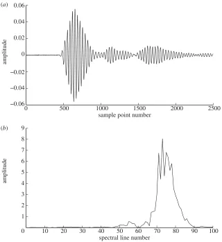
Identical piezoceramic discs were bonded at the plate edges to minimize reflections from these edges and at the mid-point of these edges to allow for greater discrimination between the direct propagating mode and its reflections from the side edges. The plate material was carbon fibre-reinforced plastic with a 0◦/90◦lay-up. Fundamental symmetric (S0) and anti-symmetric (A0) Lamb-waves were launched by driving the transmitter with a five cycle tone burst from the signal generator at 300 and 80 kHz, respectively. The signals resulting at the sensor were monitored by a digital storage oscilloscope and then transferred to PC. Figure 2 shows a typical signal in the time and frequency domains.

For this particular test, Lamb-wave signals were recorded every minute. For the first 1355 signals (a period of approx. 221₂h), the chamber temperature was held at a constant 25◦C. The temperature within the chamber was then decreased to 10◦C before being ramped to 30◦C over a 3 h period and then back to 10◦C, again over a period of 3 h. This cycling was repeated for more than three further cycles. After approximately 41 h (signal no. 2483), the chamber was opened, a 10 mm hole was drilled in the plate between the two sensors and then the chamber was closed. This essentially means that there were three different phases to the test: signals 1–1355 are from the undamaged panel held at a constant 25◦C, signals 1356–2482 are from the undamaged panel with temperature cycling and signals 2483–2944 are from the damaged panel with temperature cycling.

transmitter receiver

300

mm

damage 300mm

Figure 1. Thick composite plate (3 mm) instrumented with piezoceramic transmitter.

0 500 1000 1500 2000 2500 −0.06

−0.04 −0.02 0 0.02 0.04 0.06 (a)

(b)

sample point number

amplitude

10 20 30 40 50 60 70 80 90 100 0

1 2 3 4 5 6 7 8 9

spectral line number

amplitude

0 500 1000 1500 2000 2500 3000 1

2 3 4 5 6 7

feature number

log novelty index

Figure 3. Results of outlier analysis with training data from constant temperature samples.

lines 46–95 in figure 2), owing to their relatively higher signal-to-noise ratio and because experience has shown that damage often manifests itself through a shift in the peaks of spectral features. The feature that will be studied here, then, is the amplitude of each of these 50 spectral lines for each of the 2944 signals recorded in the test.2

In order to understand the feature data better, preliminary outlier and PCAs were carried out. For both of these, a training dataset was chosen as every second data point recorded when the temperature of the plate was held constant, in other words, taking the plate under constant temperature as the normal condition. For the outlier analysis, the mean, {¯x}, and covariance matrix, [S], were calculated for the 678 training set samples. All feature samples were then in turn designated

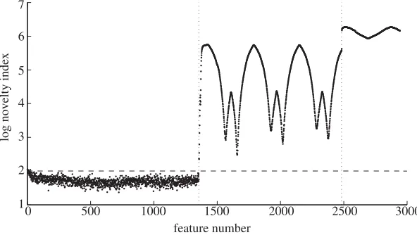
{xz} and values for Dz, the novelty index (discordancy), were calculated using equation (2.1). Figure 3 shows the results of this analysis, with novelty index being plotted on a log scale (note that the novelty indices of the samples in the training set are also plotted). The horizontal dotted line represents the threshold value, which is the critical value for a 1 per cent test of discordancy (calculated using the training data), whereas the vertical lines separate the three regimes.

Not surprisingly, almost all of the novelty indices from samples in the constant temperature regime are below the threshold. Meanwhile, the features from the temperature cycling period and the damage set are all substantially over the threshold, indicating an abnormal response from the plate for the majority of the testing period. This is clearly an undesirable situation; if the outlier analysis was to be intended as a damage detector, responses from the plate under a changing temperature would be wrongly classified as such.

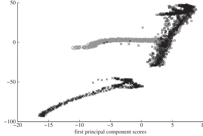
PCA is also carried out here to better understand the underlying structure of the response data from the three different regimes. A plot of the first two principal component scores is shown in figure 4, where one can see that data

from the three different regimes cluster separately, with very little overlap. The most important thing to note is that data from the undamaged response at a constant temperature do not overlie the ‘undamaged’ data from the temperature cycling period. The consequence of this, as for the outlier analysis carried out previously, is that a reliable damage indicator may not be fabricated from the constant temperature measurements alone.

Having now a clear view of the data, §4 will explore how the effects of temperature can be dealt with to create a working novelty detector.

4. Results

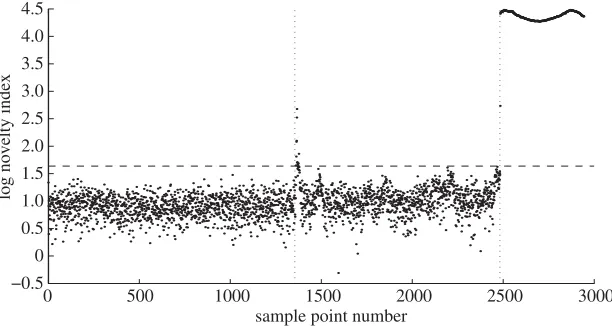
Studying figures 3 and 4 gives an insight into how badly a novelty detector would work if the constant temperature data were considered to define the normal condition; the temperature fluctuations lead to a false-positive detection of damage that is very undesirable. An obvious improvement should come from including data from the undamaged plate when the temperature was fluctuating in the training set.Figure 5shows the results of the same outlier analysis carried out in §3, with a 1 per cent discordancy threshold, this time with the training data extended to include data from the fluctuating temperature regime. Unless otherwise stated, the training dataset used in this section will be every second data point up to data point 2000; this includes data from just under two full cycles of temperature fluctuation. On inspection offigure 5, redefining the normal condition to include data points from the temperature fluctuating regime of the test has certainly decreased the discordancy of the data points from this regime; however, some structure still remains visible in the fluctuating temperature period and many points cross the threshold (indicated by the dashed line). In terms of damage detection, this outlier analysis would still be very inappropriate.

(a)Searching for damage-sensitive features that display environmental insensitivity

As discussed in §2, a possible solution is to seek out features that display insensitivity to environmental conditions but retain sensitivity to damage. Here, a univariate novelty index is used to identify the spectral lines that display a low discordancy measure under changing environmental conditions for further analysis. To do this, the mean, m, and the standard deviation,s, for each of the 50 components of a training set of features are calculated; a univariate novelty indexzz is then calculated for samples, xz, in a test set using equation (4.1)

zz=|xz−m|

s . (4.1)

Here, the training set used is the same as in the previous section, i.e. every second signal from the constant temperature period. Two test sets are used to seek out candidate features that display environmental insensitivity: the first comprises the remainder of the constant temperature signals; the second is made up of all signals from the temperature cycling period prior to the introduction of damage.

−20 −15 −10 −5 0 5 10 −100

−50 0 50

first principal component scores

second principal component scores

Figure 4. Plot of first two principal component scores, trained on constant temperature data. Circles, training data (constant temperature); diamonds, constant temperature; squares, temperature cycled undamaged; crosses, temperature cycled damaged.

0 500 1000 1500 2000 2500 3000 1.0

1.5 2.0 2.5 3.0 3.5 4.0 4.5 5.0 5.5

feature number

log novelty index

Figure 5. Results of outlier analysis using basic feature with extended training period to include temperature variations.

line at a 97% confidence limit. The dotted lines are the mean of the discordancy measures plus 1 s.d., and are added to give some idea of the variability of the relevant component within the particular testing set.

5 10 15 20 25 30 35 40 45 50 0

10 20 30 40 50 60

feature dimension number

univariate novelty index

Figure 6. Results of univariate novelty analysis for testing sets 1 and 2. Thick solid line, test-set 1 univariate outlier mean; dotted line, univariate outlier mean plus 1 s.d.; thin solid line, test-set 2 univariate outlier mean; dashed line, outlier threshold.

0 500 1000 1500 2000 2500 3000 −0.5

0 0.5 1.0 1.5 2.0 2.5 3.0

feature number

log novelty index

Figure 7. Results of outlier analysis using advanced feature calculated using univariate novelty indices.

dotted lines mark the three stages of experimental procedure. From this figure, it can be seen that the objective has very nearly been achieved; almost all of the features from the undamaged, temperature cycling set have resulted in novelty indices below the threshold, while all of the features from the damage testing set are significantly above the threshold. This shows that certain components of the original basic feature are relatively insensitive to changes in temperature but sensitive to the introduction of damage.

(b)Minor principal components for removing environmental sensitivity

While the univariate novelty index method examines to see whether there are individual components insensitive to temperature changes but sensitive to damage, the second method under investigation here seeks to find whether there exist linear combinations of the feature components that achieve the same purpose through PCA. The method for doing this is simply to perform a PCA on the training data and the first two sets of testing data (from the uniform temperature period and the cycling temperature period) and discard the higher principal components that will account for the maximum variance in the data, which is expected to be due to the temperature variations. If and when these three sets of data from the unfaulted plate cluster together, the data from the damage testing set may then be projected into the same minor component space.

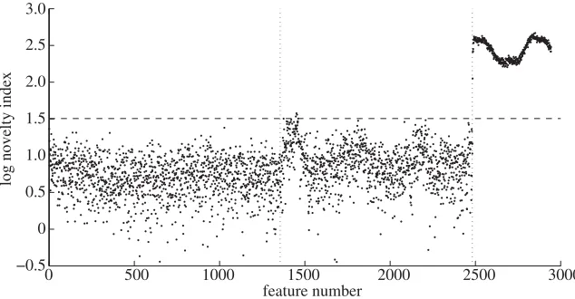
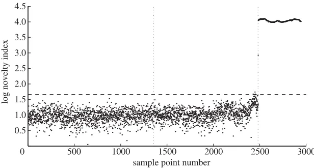
For the basic features considered here, it was found that, by examining plots of principal component n versus principal component n+1, the vast majority of the variance due to temperature change was contained in about the first 10 components. However, in order to make sure that all three sets were overlapping, only the last 10 principal components were used to form a new feature. These 10 components account for a mere 0.005 per cent of the variance in the dataset. The damage testing set was projected into the same space and an outlier analysis, with a threshold at 1 per cent discordancy, was performed using this new 10-point feature. The results shown in this section of the paper follow Manson (2002), where the principal components are calculated using every second sample of data recorded while the plate remained undamaged (both under stationary and cycling temperature); the outlier analysis uses a training dataset, as described previously, of every second sample from the stationary temperature testing period. The results are shown in figure 8, where it is obvious that this is an even more effective result than that from the previous method. All of the temperature cycled, unfaulted data have been classified as unfaulted and there does not appear to be any cyclic behaviour to the novelty indices from this set. Also, all of the damage data are very clearly classified as such. This is a very encouraging result, considering the complex nature of the data and also the temperature range considered. It should be noted, however, that the data have not been standardized prior to implementing the PCA, a fact that will be discussed further in §4c.

(c)Cointegration for the removal of environmental trends

500 1000 1500 2000 2500 3000 0

0.5 1.0 1.5 2.0 2.5 3.0 3.5 4.0 4.5

sample point number

log novelty index

Figure 8. Results of outlier analysis using advanced feature calculated using minor principal components.

and data from almost two temperature cycles.3 _{Before application, the effective} stationarity of the first difference of each feature was checked in order to meet the assumptions of the Johansen procedure. The Johansen procedure was used here to linearly combine the 50 features in question, with the aim of creating a stationary residual. If a linear combination of the training data is stationary, the common trends shared by the 50 features (i.e. the temperature-induced trends) will have been purged; any other abnormal change (such as the introduction of damage may cause) should then cause the combination residual to become non-stationary as long as each feature in question is not affected by the damage in exactly the same way.

Figure 9shows the linear combination of all 50 features for the training period chosen. The dashed horizontal lines indicate ±3 s.d. of the training data and are added to act essentially as a statistical process control X-chart (Montgomery 2009), if a data point is outside this threshold, it can be considered as abnormal. By studying figure 9, one can see that the Johansen procedure has successfully found a linear combination of the 50 features in question that is stationary over the training period, with the exception of a few points occurring around the time when the plate began to undergo its temperature cycles. This anomaly indicates that at the time of switching between the two test phases some more complex relationship between the environmental conditions and the recorded signals existed; happily after the transition period, the features returned to an equilibrium quickly and are still valid as an anomaly detector. A positive detection of damage from such an indicator would generally require a sustained excursion outside the confidence intervals, which does not occur here.

100 200 300 400 500 600 700 800 900 1000 −5

0 5 10 15 20

sample point number

residual amplitude

Figure 9. Cointegrated signal over training period (linear combination of 50 spectral lines).

0 500 1000 1500 2000 2500 3000 −250

−200 −150 −100 −50 0

sample point number

residual amplitude

Figure 10. Cointegrated signal over the whole duration of the test.

As the Johansen procedure has successfully created a stationary combination of the variables from a training set, it remains to project all of the rest of the data onto this combination and study what happens when damage is introduced. The result are shown infigure 10, where the vertical lines indicate the beginning of the temperature cycling period and the point of the introduction of damage. A clear indication of damage is apparent when the residual becomes non-stationary and deviates significantly outside the control chart boundaries (at ±3 s.d. of the training residual). Cointegration looks to be a very promising approach for the data normalization problem.

0 500 1000 1500 2000 2500 3000 −10

−5 0 5 10 15 20

sample point number

residual amplitude

Figure 11. Cointegrated signal (linear combination of 20 spectral lines).

an example, the results when including only the first 20 spectral lines from the feature set used previously are shown. Using the same training period as before, the whole 20 feature dataset projected on to the linear combination found by the Johansen procedure is shown in figure 11. As before, the dotted horizontal lines indicate±3 s.d. of the training residual, and the two vertical lines indicate the introduction of the temperature gradient and the introduction of damage, respectively. It seems that analysing a smaller subset of variables has eliminated the anomaly that previously occurred after the introduction of the temperature gradient, while the indication of damage is still very clear. Further discussion on this anomaly will follow in §5.

5. A comparison of cointegration and principal component analysis

To answer the question of how similar PCA and cointegration actually are in a mathematical way, a comparison between the set of principal components and the set of cointegrating vectors themselves should be made. The principal components in a PCA are (usually) computed using a singular value decomposition of the data matrix, and as such, the principal components form an orthogonal set. To understand the properties of the cointegrating vectors produced by the Johansen procedure, one needs to dig a little deeper into how the theory works. Without going into too much detail (see instead Johansen 1995 or Cross et al. 2011), the Johansen procedure calculates the cointegrating vectors through solving a generalized eigenvalue problem of the form

(li[N] − [M]){vi} =0, (5.1)

where{vi}is an eigenvector with corresponding eigenvalueli, and[N]and[M]are

symmetric positive definite matrices. When applying the Johansen procedure,[N] and [M] are generated from the input data and the desired cointegrating vectors correspond to the eigenvectors {vi}. The properties of a generalized eigenvalue

problem dictate that, upon solving (5.1), the resulting eigenvectors (and therefore cointegrating vectors) have an orthogonality property dictated by [N], which is that {vj}[N]{vi} =1 if i=j and 0 otherwise (Johansen 1995).

In short, the orthogonality properties of principal components and the cointegrating vectors differ (unless the matrix [N] is an identity matrix). This means that one can expect to see different results from each methodology, even though the goals of each could be viewed as being similar. To examine this, §5 provides a short comparison between results from PCA and cointegration analysis on the DAMASCOS data. How similar results from the two methodologies actually are, and which is more appropriate for the application will be explored. Within this comparison, the issue of standardizing data prior to the application of algorithms such as PCA and cointegration must be discussed. In the previous section, following Manson (2002), PCA carried out for the projection of data onto the minor components was applied without first standardizing the data. Although very good results have been produced, it is perhaps more common nowadays to standardize data before attempting PCA, so as to not form principal components biased by the size of the variables under consideration. For a complete comparison, in the following, PCA on both non-standardized and standardized data will be investigated alongside the results from applying cointegration. Using cointegration on non-standardized data is not attempted, as the Johansen procedure can easily become ill conditioned if variables of very different amplitudes are used.

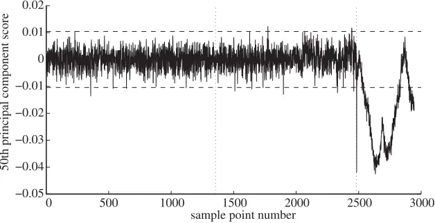
0 500 1000 1500 2000 2500 3000 −0.05

−0.04 −0.03 −0.02 −0.01 0 0.01 0.02

sample point number

50th principal component score

Figure 12. Fiftieth principal component score, PCA applied to non-standardized data.

0 500 1000 1500 2000 2500 3000 −4.0

−3.5 −3.0 −2.5 −2.0 −1.5 −1.0 −0.5 0 0.5

sample point number

50th principal component score

Figure 13. Fiftieth principal component score, PCA applied to standardized data.

The first comparison that will be made for the DAMASCOS data is between the 50th principal component score (with and without standardization of data) and the cointegrated residual from the first cointegrating vector (most stationary). For the training period described above, the 50th PC score, without prior standardization of data, is plotted in figure 12, the 50th PC score with prior standardization of data is plotted infigure 13and finally, the cointegrated residual is shown infigure 14. One could expect that the 50th principal component score, which accounts for the ‘smallest’ proportion of variance in the data would be similar to the cointegrated residual that is created using the ‘most stationary’ cointegrating vector.

0 500 1000 1500 2000 2500 3000 −120

−100 −80 −60 −40 −20 0 20 40

sample point number

residual amplitude

Figure 14. Cointegrated residual (corresponding to first cointegrating vector).

500 1000 1500 2000 2500 3000 0

0.5 1.0 1.5 2.0 2.5 3.0 3.5 4.0 4.5

sample point number

log novelty index

Figure 15. Multivariate outlier analyses of last 10 principal component scores, PCA applied to non-standardized data.

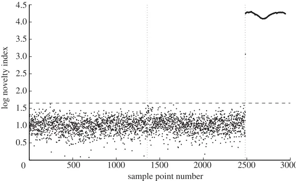
scores, trained on the same training data, will be plotted with 1 per cent discordancy thresholds. Figure 15 shows the results of a multivariate outlier analysis on the last 10 principal components from the PCA carried out on the non-standardized data, figure 16 shows the same with the PCA applied to standardized data and lastly, figure 17shows the results of an outlier analysis on the residuals created from the first 10 cointegrating vectors.

0 500 1000 1500 2000 2500 3000 −1

0 1 2 3 4 5 6

log novelty index

sample point number

Figure 16. Multivariate outlier analyses of last 10 principal component scores, PCA applied to standardized data.

0 500 1000 1500 2000 2500 3000 −0.5

0 0.5 1.0 1.5 2.0 2.5 3.0 3.5 4.0 4.5

log novelty index

sample point number

Figure 17. Multivariate outlier analyses of the residuals from the first 10 cointegrating vectors.

standardized data, figure 13, also clearly indicates the introduction of damage; on close inspection, however, the score exceeds the control chart limits during the temperature fluctuation period before damage is introduced. Lastly, the cointegrated residual in figure 14 remains within the control chart limits for the duration of the test until the introduction of damage (with one exception), where it clearly becomes non-stationary. As found previously, the cointegrated residual spikes at a time when the temperature regime was changed from stationary to cyclic.

0 500 1000 1500 2000 2500 3000 −10

0 10 20 30 40 50 60 70 80

sample point number

residual amplitude

Figure 18. Cointegrated residual created from second cointegrating vector.

From the comparisons made above, three direct observations are noted: first, that the methodologies are producing differing results; second, that it is clear that the creation of features through projection onto minor components is more successful when the data are not standardized before PCA is applied and finally, that a spike occurring at the time that the temperature cycling begins is visible in the cointegrated residuals but not in the non-standardized PCA results.

To first address the occurrence of the spike visible in figure 14(and indeed in

figure 9), it is interesting to note that upon inspection of the individual residuals created from the first 10 cointegrating vectors in the above analysis, a number of them are free from the spike in question. Although, as previously discussed, the spike does not hamper the usefulness of the residual, it seems that more suitable damage-sensitive features may be obtained that are free of it. As an example, the residual created from the second cointegrated vector is plotted in

figure 18. In this case, it seems that the ‘most stationary’ residual chosen by the Johansen procedure is not the most suitable for our cause. One should also recall that it was mentioned earlier that considering only the first 20 spectral lines of this 50 line set also produces a cointegrated residual from the first cointegrating vector that is free from the spike in question (figure 11). It seems likely that the spike is an anomaly caused by one of the variables from around the peak area of the spectrum.

From the mathematical reasoning at the beginning of this section, it is not unexpected that the results compared above are different for the two algorithms applied. For further insights, the structure of the particular combinations from each algorithm can be studied. When studying the magnitude of the coefficients for each variable (spectral line) in the combinations formed, the following observations are apparent:

— conversely, when PCA is applied to standardized data, the coefficients of the last 10 principal components are dominated by large coefficients for the spectral lines around the peak only; and

— the 10 cointegrating vectors have significant coefficients for all spectral lines, but larger coefficients have been allocated to spectral lines from around the peak area.

By not standardizing the data when calculating the principal components, precedence has been given to the spectral lines displaying a larger response magnitude than others. Consequently, the higher principal component scores will be dominated by the spectral lines from around the peak, and the lower ones the converse. If the data are standardized prior to the application of PCA, the higher principal component scores have equal contributions from each of the variables used, meaning that the contributions to the lower components are not dictated by the original amplitude of the spectral lines. Unlike the non-standardized PCA, the higher cointegrating vectors have stronger contributions from around the peak of the spectrum than from anywhere else. An explanation for this could be that the spectral lines away from the peak, that vary less, contribute less to the non-stationarity of the linear combination and as such are assigned less dominant coefficients.

From these observations, the reason that the PCA on the standardized data does not perform as well as for non-standardized data becomes clearer. By not standardizing the data, the minor component scores are dominated by spectral lines not in the peak area; these variables show lower sensitivity to temperature, and as such the temperature trend has been more easily dispersed. Where standardization has been used, this is not the case; instead, each of the principal components is dictated by the direction of the most variance in the dataset that is no longer biased by the amplitude of the spectral lines around the peak. This has, in fact, been detrimental to the performance of the minor components for the purposes of this work. That having been said, it could also be argued that the minor components of the non-standardized data are less-satisfactory candidates for damage-sensitive features due to the fact that the spectral lines around the peak, that are likely to display the greatest sensitivity to damage, have been assigned very low importance in the linear combinations. Here, one can see an advantage to cointegration, where importance is assigned to the peak spectral lines.

combinations, only certain directions in the feature space remain orthogonal. In the cointegration algorithm, the most stationary vectors are chosen first with greatest flexibility.

6. Conclusions

This study has introduced a number of methodologies for dealing with the data normalization problem in SHM in the context of data collected from a Lamb-wave inspection of a composite panel that was subjected to temperature cycling and an introduced damage scenario.

It is well know that outlier analysis is a very useful tool for novelty detection in SHM (Wordenet al.2000). However, in the face of the influence of environmental variations on damage-sensitive features, it has shown to be unreliable as a tool on its own. This paper has demonstrated (for the DAMASCOS test data at least) that other methods are necessary to account for environmental variation before outlier analysis can be implemented.

Three different approaches to finding/creating damage-sensitive features that are insensitive to environmental variations have been investigated in the paper. The first approach was an attempt to identify, without manipulation of the original variables measured, features that showed sensitivity to damage and none to environmental variations. The results for this were encouraging, in that it was possible to find some features demonstrating insensitivity to environmental conditions. Outlier analysis on these special features, although not perfect, was nevertheless successful, with very few false-positive indications of damage. Some care must be taken, however, in this approach, as most often the features that were found to be insensitive to the temperature fluctuations were those furthest away from the peak in the frequency spectrum; these points are also likely to be less sensitive to damage.

PCA has been used here both as a data visualization tool and also as a way of creating environmentally insensitive features. By projecting the Lamb-wave data onto minor principal component scores, temperature dependency has successfully been removed, which is a very encouraging result. Similarly, encouraging results have been obtained using cointegration, which finds the most stationary linear combination of variables. Both cointegration and the PCA approach have performed well in that both methods were able to create features that remained unchanged by temperature fluctuations but still were able to very clearly detect damage.

However, the dataset could still be considered somewhat removed from how data originating from a real structure in operation may appear, on account of a stationary temperature period, the lack of random variability and the fact that only one environmental factor influences the response.

The stationary temperature period in the benchmark study used here may be considered unrealistic, considering how environmental conditions for structures in operation truly vary. However, its inclusion in this work has allowed the study of response in essentially two different operating regimes, which is relevant to structures in operation. One example concerns how the response to traffic on a bridge may follow two separate regimes, one when the bridge is empty of traffic (as might occur in the very early morning) and one when traffic flows. The traffic conditions on a bridge also encompass a more rare stationary state when a traffic jam occurs and the bridge undergoes a period of constant maximal loading. A further example, perhaps more relevant here relates to aerospace SHM. A composite component on an airframe will undergo periods of non-stationarity when the aircraft is climbing or descending, but will also undergo periods of nominal stationarity while the aircraft is cruising at constant altitude and speed. Furthermore, as barely visible impact damage from tool drop during maintenance is an issue for composite structures, one may argue that monitoring should be continued when aircraft are confined in the near stationary, at least controlled, environment of a hangar. Because features for damage detection must be able to function in different operating regimes, the training data for data-based approaches should attempt to encompass all expected normal conditions, stationary and non-stationary. Nevertheless, trials have been run where the stationary temperature period was not considered in the analysis, and these have not been added here for reasons of space. Interestingly, removing the stationary temperature period does not materially affect the results of the minor component or cointegration analysis.

manipulation of a dataset. Interesting further work would be to investigate how these methodologies work in situations where the damaging event is more difficult to detect, for example, where damage is not directly on the path between the pitch and catch sensors, or where smaller or multiple damages are introduced.

In the final section, some comparisons were made between PCA and cointegration, which, on the surface of things, are similar methods, both creating linear combinations of original variables. It was found that cointegrating vectors and principal components are not necessarily similar; they are chosen on different criteria and have different orthogonality properties. On application to the DAMASCOS data investigated in this work, both approaches were successful for removing a temperature-induced trend. Interestingly, however, it was found that the linear combinations of the minor principal components relied on variables (spectral lines) from different areas of the spectrum than those in the cointegrating linear combinations.

While in this work both methods performed well, the authors believe that cointegration may prove more useful for the data normalization problem. As principal components are always orthogonal, after the first PC is chosen to account for the most variance in a dataset, the directions of the remaining principal components are then constrained by this orthogonality condition. As such, the minor components may not provide optimal results for removing environmental trends. It is here that cointegration may have the advantage due to the fact that the first cointegrating vector is chosen to be the most stationary, and is not dictated by any other constraints.

The authors thank all of the partners involved in the DAMASCOS consortium, the EPSRC for funding this research and finally the reviewers for their helpful and constructive comments.

References

Cross, E. J. & Worden, K. 2012 Cointegration and why it works for SHM.J. Phys. 382, 012046. (doi:10.1088/1742-6596/382/1/012046)

Cross, E. J., Worden, K. & Chen, Q. 2011 Cointegration: a novel approach for the removal of environmental trends in structural health monitoring data. Proc. R. Soc. A467, 2712–2732. (doi:10.1098/rspa.2011.0023)

Dickey, D. A. & Fuller, W. A. 1979 Distribution of the estimators for autoregressive time series with a unit root.J. Am. Stat. Assoc.74, 427–431.

Dickey, D. A. & Fuller, W. A. 1981 Likelihood ratio statistics for autoregressive time series with a unit root.Econometrica49, 1057–1072. (doi:10.2307/1912517)

Johansen, S. 1995Likelihood-based inference in cointegrated vector autoregressive models. New York, NY: Oxford University Press.

Juselius, K. 2006The cointegrated VAR model: methodology and applications. Oxford, UK: Oxford University Press.

Kullaa, J. 2004 Structural health monitoring under variable environmental or operational conditions. In Proc. 2nd European Workshop on Structural Health Monitoring, Munich, 7–9 July 2004(eds C. Boller & W. J. Staszewski). Lancaster, PA: DEStech Publications. Manson, G. 2002 Identifying damage sensitive, environment insensitive features for damage

detection. In Proc. 3rd Conf. on Identification in Engineering Systems, University of Wales, Swansea.

Sharma, S. 1995Applied multivariate techniques. London, UK: John Wiley & Sons, Inc.

Sohn, H. 2007 Effects of environmental and operational variability on structural health monitoring.

Phil. Trans. R. Soc. A 365, 539–560. (doi:10.1098/rsta.2006.1935)

Sohn, H., Dzwonczyk, M., Straser, E. G., Law, K. H., Meng, T. & Kiremidjian, A. S. 1998 Adaptive modeling of environmental effects in modal parameters for damage detection in civil structures. InProc. SPIE 3325, Smart Structures and Materials 1998: Smart Systems for Bridges Structures and Highways(ed. S. Liu), pp. 127–138. Bellingham, WA: SPIE.

Stock, J. H. & Watson, M. W. 1988 Testing for common trends.J. Am. Stat. Assoc.83, 1097–1107. (doi:10.1080/01621459.1988.10478707)

Stock, J. H. & Watson, M. W. 1993 A simple estimator of cointegrating vectors in higher order integrated systems.Econometrica61, 783–820. (doi:10.2307/2951763)

Worden, K., Manson, G. & Fieller, N. R. J. 2000 Damage detection using outlier analysis.J. Sound Vib.229, 647–667. (doi:10.1006/jsvi.1999.2514)