Abstract: Capturing public insights related to transit systems in social media has gained huge popularity presently. The regional transportation agencies use social media as a tool to provide information to the public and seek their inputs and ideas for meaningful decision making in transportation activities. This exploratory study attempts to gauge the impact of social media use in transportation planning that in turn would help transportation administration in identifying the day-to-day challenges faced by the customers and to suggest a suitable solution. This paper presents the effect of pre-processing techniques on transit opinion analysis to improve the performance. Performance of different pre-processing methods namely stop word removal, stemming, lemmatization, negation handling and URL removal using feature representation models namely TF-IDF with unigram, TF-IDF with bigram on three feature selection techniques including information gain, standard deviation and chi-square on social media transit rider’s opinion is carried out. The experimental results are evaluated using four different classifiers such as Support vector machine, Naïve Bayes, Decision Tree, K-Nearest Neighborhood in terms of accuracy, precision, recall, and f-measure. On analyzing the social media related transit opinion data, it is observed that pre-processing with bigram technique performs better than the other approaches specifically with Support Vector Machine and Naïve Bayes.
Keywords: Feature selection, Machine learning, Opinion mining, Text pre-processing, Twitter, Transit opinion analysis, Social media.
I. INTRODUCTION
The use of social media in public transportation has gained enormous development in this digital era in terms of efficiency. Transportation organization raises the economic growth with the perspective of the well-being of users using social media as a platform, who share their opinions, access the employment, services and social connections. Transportation stakeholders not only forecast the ups and downs occurring in the transportation domain but also understand the customer's expectations and needs in terms of quality of services on exploring the reasons for facing dissatisfaction. Transportation-related data in social media has gained significant importance in transportation research. The Natural Language Pre-processing and sentiment analysis
Revised Manuscript Received on November 05, 2019.
* Correspondence Author
Meesala Shobha Rani, School of Computer Science and Engineering,
Vellore Institute of Technology, Vellore, India. Email:
Sumathy.S*, School of Information Technology and Engineering, Vellore Institute of Technology, Vellore, India. Email: [email protected]
techniques are applied in the domain of transportation for transportation tweet assessment. The major concern faced by railways today is its ineffectiveness to meet the requests of its customers. In addition, the quality of services is monitored continuously by users and their opinions are posted on social media cleanliness, timeliness of administrations, security, nature of terminals, dimensions of trains, quality of food, the security of travelers and facility of booking tickets are issues that require demanding consideration.
With an increase in the evolution of online social networks, social media has become an emerging area in handling massive input and output of user-generated information. Today, the predominant type of investigation of social media information depends upon text mining and natural language processing techniques such as sentiment analysis. Public transportation tweet analysis is used to study traveler opinions, sentiments, attitudes, emotions, evaluation towards certain aspects of traffic-related features and to classify traveler’s responses as positive or negative.
Tweets are typically made of incomplete, noisy, unstructured sentences, not well-shaped words, unpredictable articulation and non-lexicon terms. Though numerous algorithms for the detection of opinion analysis on huge datasets with the extraction of sentiment features to perform various performance analyses are proposed by researchers, efficient schemes to select suitable pre-processing methods is not addressed much. Pre-processing is a method of removing noisy data and preparing the text for classification. Prior to performing feature selection, sequences of text pre-processing methods (stop word removal, lemmatization, stemming, URL removal and negation handling) are used to remove noise in the tweets.
This paper presents the comparison of various text pre-processing methods on social media transit opinion analysis. The feature representation models namely, TF-IDF using unigram and bigram and classifiers such as SVM, NB, DT, and KNN are used to classify sentiment polarity on the social media transit opinions. Out of 168 combinations of commonly used techniques on transit dataset for opinion analysis, the results show that the significance with pre-processing using bigram achieves better classification performance and is used to analyze and identify public attitudes or opinions towards transportation activities effectively.
Opinion Mining on Social Media Transit Tweets
using Text Pre-Processing and Machine
Learning Techniques
The rest of this paper is organized as follows: Section 1 presents the introduction and section two discusses the related research on social media transit tweet analysis, pre-processing techniques for sentiment analysis. Section three highlights the research gaps in the domain of interest. Section four presents the methodology of social media related transportation tweet analysis is presented in section four and experimental results are in section five. Discussions and comparative analyses are provided in section six. Conclusion and future work presented in section seven.
II.
RELATED RESEARCH
A. Social Media in transportation tweet assessment [1] Presented a methodology for the automatic extraction of transportation-related information from TripAdvisor. [2] Proposed a deep learning approach for detecting accidents using social media data. [3] Presented a fuzzy ontology-based opinion mining of transportation city features such as bus and train stations, parks, restaurants, etc., for safe and secure traveling and for increasing the transportation facilities. [4] discussed a methodology that scrutinizes and visualizes the geotagged social media data to know the destination choice and business clusters. [5] Presented a case study on the investigation of social media approaches for transportation information management during the commonwealth games. [6] Presented a methodology for collecting public insights from social media. The proposed approach is pragmatic to a case study on the bus rapid transit system in Colombia. [7] Studies the traveler insights of destination amenities through the hybrid approach of visitor’s online reviews by using sentiment analysis and co-occurrence analysis. [8] Presented a methodology and highlights the challenges faced in the extraction of transportation-related information from social media and an investigation of Twitter messages for identifying the transportation-related social media tweets. [9]-[11] Presented a methodology for stakeholder sentiment classification which identifies the opinion of the stakeholders during the large-scale transportation project at initial stages. [12][13] Discussed the extraction of various aspects of transportation information from social media, which is examined and revised based on human perceptions. [14] Proposed a methodology that explores the abilities to make use of geotagged social media twitter data and investigate the longitudinal travel behavior analysis. [15] [16] Presented an approach that integrates the text mining techniques and ensemble methods which increases the performance of models for predicting the severity of rail accidents. [17] Explores the prediction of transportation sentiment classification using Instagram social media features. The combination of visual and textual features increases the accuracy of predicting transportation sentiment classification. [18] Proposed a methodology for creating the transportation ontologies and semantic services for extracting the transportation-related information which is used in the intelligent transportation system domain.
[19] Presented an approach for the detection of real-time traffic events using social media tweets. The methodology is applied to two metropolitan regions. [20] Presented an
approach for identifying and detecting the railway safety assessment and risk circumstances using big data analytics. [21] Discussed an approach for extracting the information from social media and developed an innovative product and services for the transportation domain using automated content analysis. [22] [23] Discuss big data analytics to simplify social media mining and estimation on the improvement of rail service performance. [24] Presented a topic modelling and unsupervised machine learning method for transit services using social media related transit data. [25] Presents the challenges faced in large scale transportation operations in Indian railways. [26] Presented a survey using social media on collecting transportation information, creating transportation lexicon, transportation planning, operations, opportunities and challenges in transportation domain.
B. A review of pre-processing techniques using sentiment analysis
A methodology on the comparison of text pre-processing techniques using twitter datasets for sentiment classification are presented in [27]-[31]. [32] Discuss a methodology for handling negation sentiment analysis at sentiment level. [33] Proposed an approach using clustering algorithms for document sentiment classification. [34] Proposed a framework using text pre-processing and n-gram to find slang words in twitter sentiment classification. [35] Proposed a methodology on parallel implementation of text pre-processing techniques for sentiment classification using the twitter dataset. [36] Discussed a methodology on Arabic sentiment classification using text pre-processing, n-gram and machine learning techniques. [37] Presented an approach for sentiment classification using text pre-processing techniques, feature representation and support vector machine on movie reviews. [38] Proposed a methodology on the integration of unigram, bigram, NB and maximum entropy for text pre-processing sentiment classification on twitter dataset. [39] Presented an approach for accumulating and executing the geo-tagged tweets. [40], [41], [42] Discussed a twitter brand sentiment classification using n-gram and statistical schemes.
III. RESEARCHGAPS
A methodology of text mining with a combination of techniques to automatically detect the accident severity is [16] presented. It requires probabilistic models for assessing accident severity.
A methodology of Tensistrength approach to detect stress and relation views in the social media text [43]. The performance of Tensistrength is less compared to the generic machine learning techniques based on unigram, bigram, and trigram. Focus on reduced feature size with an emphasis on increasing performance is required.
It requires normalization of tweets as well as the removal of stop words.
IV. SOCIALMEDIATRANSITTWEET ASSESSMENT
Raw data (transportation tweets) is used to build public transportation tweet analysis. The partial noise and incompatible data are removed by incorporating text pre-processing and natural language processing techniques. Through pre-processing, tweets are normalized and transformed into a vector representation. Each tweet of the raw data is represented in terms of row values for each feature. The input vectors are fed into each feature selection phase and are used for extracting the relevant and useful terms for training the classifier model. These feature values are used as input for each of the machine learning classifiers. The output of the classifiers is used for classifying the transportation tweet as either a positive or a negative tweet.
A. Transit tweet collection
Twitter allows accessing only 1% of its tweets through streaming Twitter API due to its boundaries of company policies. However, researchers prefer real-time datasets for experimentation. Hence, the available transportation-related tweets are used as the only source. Research mainly focuses on the streaming of transportation tweets analysis which can be accessed and determined from Twitter. As Twitter does not automatically label the huge amount of user-generated data, physical labelling is performed. The transportation dataset extracted contains 11000 tweets from India during 2017 over the course of 30 days’ time frame. Tweets are accumulated using the Twitter Streaming API from @RailMinIndia. Tweets are extracted and stored in CSV format which contains text, favorite count, reply to screen name, created, truncated, reply to Sid, id, reply to the user id, status source, screen name, retweet count, is a retweet, retweeted, longitudes and latitudes. The reviews or tweets are selected from the downloaded twitter information. For example, consider a mining railway transportation tweet from social media: ―@RailMinIndia Really a proud moment. pls, carry forward all good works of your predecessor‖.
B. Text pre-processing techniques for transit tweet analysis
Raw data is accumulated and pre-processing is applied. The input data must be clean from punctuation marks such as numbers, symbols, commas, punctuations, periods and convert upper case to lower case. The pre-processing task incorporates cleaning, tokenization, normalization, removal of stop words, stemming, lemmatization, negation handling and removal of URL links in the text.
Stop word removal:Stop words are words such as ―the‖,
―i‖, ―we‖, ―a‖, ―and‖ etc., which are removed in the pre-processing stage. These words occur frequently in the sentence which has no meaning and affects the classification performance.
Stemming: Stemming is the process of removing the inflected word in order to detect the root word. For example: ―@drashok08 @RailMinIndia @nr_ctg @PiyushGoyal PCM has been advised to attend you
immediately‖. Immediately is stemmed into immediate, advise is stemmed into advice. All stemmed words are grouped into one bucket form to reduce the dimensionality of words. Stemming increases the classification performance. The porter stemmer algorithm is used in the proposed methodology.
Lemmatization: Lemmatization is the process of converting inflected words to the root form. For example ―drove‖ is converted into ―drive‖.
Negation handling: Generally, negation plays an important role in sentiment classification. For example: ―The journal wasn’t good it was horrible‖. Neglecting the negated words causes misclassification and results in poor performance. Negation words (won’t, can’t, shouldn’t, couldn’t, wouldn’t, hadn’t, hasn’t, haven’t, etc.,) is replaced with not.
URL Removal:Most of the twitter information contains a URL and an https link. It does not contain any meaning in the sentiment. Removing the URLs from the twitter information refines the tweets. For
example:‖ @oneindiaHindi @PiyushGoyal
@PiyushGoyalOffc @RailMinIndia Plz check the behavior of tt of train no. 12872 from sb… https://t.co/Su8b4MQGkO‖.
C. Term frequency-inverse document frequency (TF-IDF)
The vector space model has frequently used representation in text processing. In the feature transformation phase, tweets are represented via the vector space model associated with the TF-IDF scheme. The tweets or opinion (R) is represented as vector Rj = (w1j, w2j, w3j,…….wtj) and the individual
dimension corresponds to a separate word (w) or term for the opinion j. Term frequency measures the frequency of the term in a document [44][45]. Term frequency of tf is defined as follows,
tfij = nij/Nj (1)
Where nij is the number of times term i occurring in tweet j
and Nj is the total number of terms in tweet j. Inverse
document frequency (IDF) measures the importance of a term in the dataset,
idfi= log(D/di) (2)
in which, d is the number of tweets in which the term i occurs and D is the total number of tweets. The TF-IDF is the most extensively accepted term weighting scheme used in information retrieval and text mining. It measures the significance of a specific word in the document as well as in the corpus through inverse document frequency.
tf idf = tfij * idfi (3)
Where tfij is the term frequency of term i and idfi is the inverse
D. N-gram model
N-gram is a probabilistic language model extensively used in
sentiment classification. It is mostly used to measure a contiguous sequence of sentence or words in the corpus, where N is the sequence of words (n=1) unigram, (n=2) bigram, (n=3) trigram [41],[42],[46]. For example: ―@RailMinIndia Sir ―local‖ ―train is‖ ―scheduled very late‖. Pls, focus on train timings very poor service in NR special Delhi to Ghaziabad‖. The word unigram is ―local‖, bigram is ―train is‖ and tri-gram is ―scheduled very late.E. Chi-Square (χ2)
Chi-Square test is a statistical measure that estimates the dependence between a feature and a class. The higher value of chi-square states that the related class is more dependent on the available feature which implies that a lower value of chi-square must be removed as it contains less information [47]. It is applied for text mining, where terms or words or N-gram are features. The 2-by-2 contiguous table for feature f and class c is defined as follows:
χ2 = (4)
where P is the number of documents in class c that contains feature f, Q is the number of documents in alternate class that contains f, R is the number of documents in class c that does not contain f, S is the number of documents in an alternate class, that does not contain f, and N is the aggregate number of documents.
F. Information Gain
The most common feature selection method for sentiment analysis is information gain. This method determines the information content after getting the value of a feature in a document. The higher score of information gain facilitates discrimination between different classes. The entropy value is defined by the uncertainty of the probability distribution for the given classes. Consider m to be the number of classes in C = {c1,c2…..cm}where the entropy can be defined as [47],
H (C) = (5)
Where is the probability of a number of documents in class ci. If an attribute A has n distinct values A = {a1, a2, ……
an} then the entropy after the attribute A is observed as
follows
H (C|A) = (6)
Where the probability of the number of documents containing the attribute value and is the probability of the number of documents in class that contains the attribute value Information gain is defined based on the difference in entropy values before and after the attribute observation as
IG (A) =H (C) – H (C|A) (7)
G. Standard Deviation
Standard deviation is the probabilistic and statistical measure that estimates the deviation or variation of features. The low
standard deviation shows that a feature point tends to be close to the mean and the high standard deviation shows that the feature points are extended out over a large range of values. Let D={d1,d2,d3….dN}the set of documents, where di is the
document and l ={l1,l2,l3……lN}is the label set of documents
used for sentiment classification, li=+1 represents the positive
sentiment of the text document and the negative sentiment of the text document represents li=-1. Let (li, di) be the training
set of classifiers used for predicting unknown label documents [48]. The standard deviation is calculated as follows
j = ij where j=1…..M (8)
SDj= where j=1…..M (9)
Where fij signifies the weight of jth feature measured by the
TF-IDF scheme to the ith document, j indicates the mean or
average of jth feature, SDj indicates the standard deviation of
the jth feature, M signifies the number of features and N signifies the number of documents.
H. Naïve Bayes
Naïve Bayes classifier is a popular and effective algorithm used for text classification. The bayesian probabilistic model assigns a posterior class probability to an instance and follows Bayes rule for generating the documents. Let Y be the class label, X be the projection of tweet into a feature vector X = [X1, X2…… XN], N is the dimension of the feature vector,
where the total number of words and combinations in the corpus is positively correlated with the event. The Bayes theorem is used to estimate the conditional probability as follows [49],[8].
(10)
Where P(Y) is the probability of a class, P (X|Y) is the conditional probability. To simplify the joint conditional probability , X has high dimensional feature vectors. To reduce the complexity of high dimensionality, Naïve Bayes classifier assumes the conditional independence of all features such that they are conditionally independent of one another.
(11)
which can be further simplified as
(12)
where all features are sorted in the order, in which correlated feature instances stay first and independent features follow them. The correlated instances are indicated by the symbol in the first and the last positions and the j th to ith positions indicate independent features. Probability of a set of instances of all feasible instances of a class variable y* is estimated and the output with maximum probability is determined as
I. Support Vector Machine
The support vector machine is a powerful supervised machine learning algorithm for text and sentiment classification. It separates the training data instances into binary classes using the decision boundaries. The decision depends on the support vectors that are the only selected efficient instances in the training dataset. SVM is originally designed for binary class problems that deal with maximizing the margin and separating the hyperplane between two data instances. Let X be the labeled training feature vectors (x1,y1),….(xn, yn), and
each training instance xi ϵ RN is designated label as yi ϵ {-1,
+1} where i=1…..n. The aim is to compute f(n)= w. xi +b and
to identify a classifier y(x)= sign(f(x)) that can be interpreted through the convex optimization as follows [47],
(14)
Where isthe regularization parameter, xi is the feature
vector, yi ϵ{-1, +1}, w is the normal vector to the hyperplane
and b is the offset of the hyperplane.
J. K-Nearest Neighbor
K-Nearest Neighbor classification is known to be the simplest lazy machine learning algorithm which is an instance-based learning technique that focuses on classifying the objects based on predefined classes on basic sample groups using Euclidian distance. This method does not require training data in order to classify data, however training data are used during testing. The algorithm classifies documents in a Euclidian space as points. The Euclidian distance d between two points is as follows [50].
(15)
Where d is the distance, X1= (x11, x12, x13, …. x1n) , X2 = (x21,
x22, x23…. x2n), n is the number of documents.
K. Decision Tree
Decision tree induction is the learning of decision trees from class labeled training instances. The structure of the decision tree doesn’t require any domain knowledge or parameter setting. A decision tree is robust to noise and handles multi-dimensional data, where each internal node represents a test on an attribute, each node represents an outcome of the test and each leaf node represents a class label. The algorithm starts with instances in the training set and selecting the best instances yielding significant information for classification [51], [52],[47].
V. EXPERIMENTALANALYSIS
The experiment is carried out using MATLAB R2017b on HP laptop i5 processor; 8GB RAM with accumulated tweets from social media transportation-related tweets. The Twitter corpus such as emotions as noisy unstructured tweets, irrelevant expressions, stop words, URLs, and retweets were collected using Twitter Streaming API. The corpus contained 11000 social media transportation tweets. Manual annotation as positive and negative sentiment based on the public attitude was performed. For sentiment classification four well-known machine learning classifiers namely SVM (RBF kernel), Naïve Bayes, DT (C4.5) and KNN are set as default
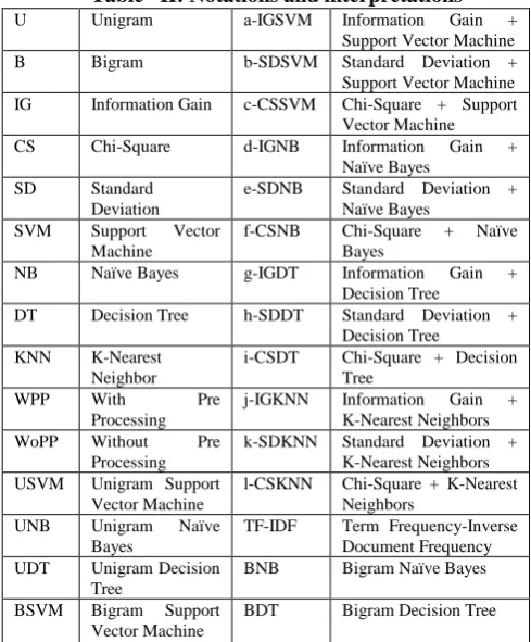
[image:5.595.304.549.256.324.2]parameters. The positive tweet containing a high favorite count tends to be a more positive tweet. The negative tweet containing a high favorite count tends to be a more negative tweet. The pre-processing, term weighting and n-gram model, feature selection and machine learning techniques are evaluated on twitter corpus. The experiment is performed on all combinations. Performance metrics such as accuracy, precision, recall, and f-measure is presented from Fig.1 to Fig.14. The confusion matrix is shown in Table I[3], where TP, TN, FP, and FN represent true positive, true negative, false positive and false negative in the information retrieval. Precision is defined as a number of retrieved elements that are relevant. The recall is defined as a number of relevant elements that are retrieved. F- Measure is the harmonic mean of both precision and recall. Accuracy is the amount of total detection rate. Table II provides the notations used in the graph.
Table-I: Confusion matrix
VI. DISCUSSIONANDCOMPARATIVEANALYSIS
[image:5.595.304.549.396.692.2]The experimental results show that the performance of sentiment classification varies based on classifiers used.
Table –II: Notations and interpretations
U Unigram a-IGSVM Information Gain +
Support Vector Machine
B Bigram b-SDSVM Standard Deviation +
Support Vector Machine
IG Information Gain c-CSSVM Chi-Square + Support
Vector Machine
CS Chi-Square d-IGNB Information Gain +
Naïve Bayes
SD Standard
Deviation
e-SDNB Standard Deviation +
Naïve Bayes
SVM Support Vector
Machine
f-CSNB Chi-Square + Naïve
Bayes
NB Naïve Bayes g-IGDT Information Gain +
Decision Tree
DT Decision Tree h-SDDT Standard Deviation +
Decision Tree
KNN K-Nearest
Neighbor
i-CSDT Chi-Square + Decision
Tree
WPP With Pre
Processing
j-IGKNN Information Gain +
K-Nearest Neighbors
WoPP Without Pre
Processing
k-SDKNN Standard Deviation +
K-Nearest Neighbors
USVM Unigram Support
Vector Machine
l-CSKNN Chi-Square + K-Nearest
Neighbors
UNB Unigram Naïve
Bayes
TF-IDF Term Frequency-Inverse
Document Frequency
UDT Unigram Decision
Tree
BNB Bigram Naïve Bayes
BSVM Bigram Support
Vector Machine
BDT Bigram Decision Tree
Fig.1 shows the experimental results obtained from the social media railway transportation-related tweets. It is observed that the highest accuracy is achieved by using Stop word Removal+ Unigram+ CS+KNN, where accuracy is 81.38%,
Information retrieval Relevant Irrelevant
Retrieved TP FP
precision is 81.77%, recall is 99.37% and f-measure is 89.71%. In SVM, using stop word removal, unigram and CS achieves better classification performance. NB achieves poor performance results in all approaches. In DT, using stop word removal, unigram and IG achieves better performance.
Fig.1. comaparison of stop word removal using unigram
Fig.2. Comparison of stop word removal using bigram
Fig.2 represents the detailed results of stop word removal using bigram with different feature selection and machine learning techniques. A comparison of the results from the corpus revealed that the highest accuracy and precision rate of Stop word removal+ Bigram SD+SVM, Stop word removal+ Bigram CS+SVM, Stop word removal+ Bigram IG+NB, Stop word removal+ Bigram SD+NB, Stop word removal+ Bigram CS+NB are similar in terms of accuracy (81.78%) and precision (81.78%) .In contrast Stop word removal+ Bigram+ IG+SVM achieves the highest recall is 99.93% and f-measure is 89.94%. In SVM and NB, using Stop word removal, bigram, and feature selection techniques achieves better and similar classification performance. In DT, using stop word removal, bigram and SD achieve equal outcomes. In KNN using stop word removal, bigram and SD achieves similar results. Stop word removal using bigram achieves better performance compared to stop word removal using unigram.
Fig.3. Comparison of stemming using unigram
Fig.3 presents the comparison results of stemming using unigram. Stemming + Unigram +CS+KNN achieve the highest accuracy (81.61%), recall (99.71%) and f-measure (90.11%). In contrast, Stemming + Unigram+ CS+NB achieves highest precision rate (82.33%). In SVM, using stemming, unigram and SD achieves better performance results. NB achieves poor accuracy performances. In DT, using stemming, unigram and SD achieves better performance results. In KNN, using stemming, unigram and CS achieves better performance results. Stop word using unigram gives more impact on classification performance compared to stemming using unigram.
Fig.4. Comparison of stemming using bigram
Stop word using bigram, and stemming using bigram provides equally comparable results.
Fig.5 describes the comparison results of lemmatization using unigram.Lemmatization+ Unigram+ SD+NB achieved the highest accuracy (81.76%), precision (81.77%), recall (99.97%) and f-measure (89.95%). In SVM using lemmatization, unigram and SD achieves better performance. In NB, using lemmatization, unigram and feature selection achieves better classification performance. In DT, using lemmatization, unigram and SD achieves better performance. In KNN, using lemmatization, unigram and CS achieves better performance.
Fig.5. Comparison of lemmatization using unigram
Fig.6. Comparison of lemmatization using bigram
Fig.6 illustrates the detailed results of lemmatization using bigram. Lemmatization+ Bigram+ IG+NB, Lemmatization+ Bigram+ SD+NB, Lemmatization+ Bigram+ CS+NB achieve the similar highest performance in terms of accuracy (81.78%), precision (99.90%), recall (99.97%) and f-measure (99.93%). In SVM, using lemmatization, bigram and feature selection techniques gives equally comparable results. In NB, using lemmatization, bigram, and feature selection techniques gives similar classification performance results. In DT, using lemmatization, bigram and SD gives better performance. In KNN, using lemmatization, bigram and feature selection techniques gives better performance results. Lemmatization gives less impact on classification performance compared to stop word removal and stemming. Lemmatization using
bigram achieves better results compared to using unigram.
Fig.7. Negation handling using unigram
Fig.7 highlights the performance results of negation handling using unigram. Negation handling+ Unigram+ SD+KNN achieves the highest accuracy (81.32%), recall rate (99.22%) and f-measure (89.67%) compared to other approaches. In contrast, Negation handling+ Unigram+ CS+NB achieves the highest precision rate of 83.44%. In SVM, using Negation replacement, unigram and SD achieves better classification results. NB achieves less classification accuracy compared to other approaches. In DT and KNN using negation, unigram and SD gives better results.
Fig.8. Comparison of negation handling using bigram
In SVM, DT and KNN using negation, unigram and SD give similar performance results. NB results in poor accuracy. Negation replacement using unigram approaches have less impact on tweet classification compared to lemmatization using unigram approaches. Negation handling using bigram achieves better results compared to negation handling using unigram.
Fig.9. Comparison of URL removal using unigram
Fig.9 presents the performances of URL removal using unigram. URL removal+ Unigram+ SD+KNN achieves the highest performance compared to other approaches in terms of accuracy (81.45%), recall (99.60%) and f-measure (89.77%). In contrast, URL removal+ Unigram+ SD+NB achieves highest precision of 82.78%. In SVM, DT and KNN on removing URL, unigram and SD gives a better classification performance. NB achieves low-performance results.
Fig.10. Comparison of URL removal using bigram
Fig.10 depicts the comparison of URL removal using bigram. URL removal+ Bigram+ IG+NB achieves the highest accuracy (81.78%), precision (81.78%), recall (99.97%) and f-measure (99.93%). URL removal has significant importance in tweet analysis compared to stop word removal, stemming, lemmatization and negation handling. URL removal using unigram and bigram shows similar performance in all individual cases.
Fig.11 presents the comparison of pre-processing using
unigram. In SVM and DT, using pre-processing techniques, unigram and SD gives similar accuracy classification results. In NB, using pre-processing techniques with unigram and feature selection techniques gives better results compared to other with pre-processing using unigram approaches. In KNN, using pre-processing techniques, unigram and CS gives better classification performances. Applying the pre-processing (stop word removal, stemming, lemmatization, negation handling and URL removal), feature selection techniques(IG, SD, CS) to SVM, NB, DT and KNN, it is observed that SDNB achieves better performance in terms of accuracy (81.74%), recall (99.95%) and f-measure (89.96%). With respect to precision value (81.97%), CSSVM achieves better results. The proposed methodology is compared to the existing approaches (USVM, UNB, and UDT) in terms of precision, recall and f-measure rate, where UNB achieves a better precision rate (84%) compared to other approaches
Fig.11. Comparison of with pre-processing using unigram
Fig.12. Comparison of with pre-processing using bigram
In SVM and NB, using pre-processing techniques with bigram and feature selection techniques gives the highest classification performance compared to all other approaches. DT and KNN give the moderate classification performance. Applying the pre-processing (stop word removal, stemming, lemmatization, negation handling and URL removal), feature selection techniques (IG, SD, CS) to SVM, NB, DT and KNN, it is observed that CSSVM gives better performance in terms of accuracy (99.98%), precision (99.98%), recall (99.97%) and f-measure (99.97%). The proposed methodology is compared to the existing approaches (BSVM, BNB, and BDT) in terms of performance metrics such as precision, recall and f-measure rate, where BSVM and BNB give better precision rate (88% and 97%) compared to the other approaches.
Fig.13. Comparison of without pre-processing using unigram
Fig.13 presents the comparison of without pre-processing using unigram. In SVM, using unigram and IG gives better classification performance. In NB, using unigram and feature selection techniques gives low accuracy performance in all cases. In DT, using unigram and SD gives moderate classification performance. In KNN, using unigram and feature selection techniques gives similar performance results in all cases and gives better performance compared to other approaches. Lack of pre-processing techniques gives low-performance classification. The raw tweets were tokenized into sentences and then into words. The tokenized tweets are transformed and normalized into a unigram vector space. The input vectors are fed to the feature selection techniques IG, SD, and CS. The features selection values are used as input to the four machine learning classifiers: SVM, NB, DT, and KNN. It is observed that IGKNN achieves the highest performance in terms of accuracy (80.94%), precision (81.73%), recall (98.77%), and f-measure (89.43%) compared to other classifiers. The proposed methodology (without pre-processing using unigram) is compared with existing approaches (USVM, UNB, and UDT) in terms of precision and recall and f-measure, where UNB achieves better precision rate (84%) compared to other approaches. Overall, it is observed that with pre-processing using bigram achieves better performance results compared to with
pre-processing using unigram and existing approaches. Fig.14provides a comparison without pre-processing using bigram. In SVM,NB, DT, and KNN using bigram and feature selection techniques give similar performances. The tokenized tweets are transformed and normalized into a bigram feature space and are fed into the feature selection phase. The features selection values are used as input to the four machine learning classifiers: SVM, NB, DT, and KNN. It is observed that SVM and NB using feature selection techniques achieve a similar classification performance in terms of accuracy (81.78%), precision (81.78%), recall (99.97%) and f-measure (89.96%) compared to DT and KNN. To evaluate the effectiveness of the comparison of various approaches, precision, recall, and f-measure are determined with and without pre-processing of unigram and bigram. The existing methodology [8] incorporates unigram using SVM, unigram using NB, and unigram using DT. Overall, it is observed that without pre-processing using bigram achieves better performance results compared to without pre-processing using unigram.
Fig.14. Comparison of without pre-processing using bigram
As a summary, it is observed that pre-processing using bigram achieves an improved performance compared to all other approaches in identifying traveler opinion analysis in terms of better accuracy, precision, recall and f-measure.
VII. CONCLUSION
Analysis of unigram and bigram using pre-processing, N-gram, feature selection, and machine learning techniques were applied to all combinations. It is observed that pre-processing using bigram achieves better performance in terms of accuracy (99.98%), precision (99.98%), recall (99.97%), and f-measure (99.96%) compared to the approach without applying pre-processing techniques to unigram and bigram. As a further enhancement, geo-tagged longitudinal tweets can be incorporated to monitor real-time traveler behavior analysis and crowd sourcing can be used to annotate the tweets in order to reduce the time and human effort.
REFERENCES
1. A. Gal-Tzur, A. Rechavi, D. Beimel, and S. Freund, ―An improved
methodology for extracting information required for transport-related decisions from Q&A forums: A case study of TripAdvisor,‖ Travel Behav. Soc., vol. 10, no. September 2017, pp. 1–9, 2018.
2. Z. Zhang, Q. He, J. Gao, and M. Ni, ―A deep learning approach for
detecting traffic accidents from social media data,‖ Transp. Res. Part
C Emerg. Technol., vol. 86, no. May 2017, pp. 580–596, 2018.
3. F. Ali, D. Kwak, P. Khan, S. M. R. Islam, K. H. Kim, and K. S. Kwak,
―Fuzzy ontology-based sentiment analysis of transportation and city
feature reviews for safe traveling,‖ Transp. Res. Part C Emerg.
Technol., vol. 77, pp. 33–48, 2017.
4. A. Huang, L. Gallegos, and K. Lerman, ―Travel analytics:
Understanding how destination choice and business clusters are
connected based on social media data,‖ Transp. Res. Part C Emerg.
Technol., vol. 77, pp. 245–256, 2017.
5. C. Cottrill, P. Gault, G. Yeboah, J. D. Nelson, J. Anable, and T. Budd,
―Tweeting Transit: An examination of social media strategies for
transport information management during a large event,‖ Transp. Res.
Part C Emerg. Technol., vol. 77, pp. 421–432, 2017.
6. I. Casas and E. C. Delmelle, ―Tweeting about public transit —
Gleaning public perceptions from a social media microblog,‖ Case
Stud. Transp. Policy, vol. 5, no. 4, pp. 634–642, 2017.
7. K. Kim, O. joung Park, S. Yun, and H. Yun, ―What makes tourists feel
negatively about tourism destinations? Application of hybrid text
mining methodology to smart destination management,‖ Technol.
Forecast. Soc. Change, vol. 123, pp. 362–369, 2017.
8. T. Kuflik, E. Minkov, S. Nocera, S. Grant-Muller, A. Gal-Tzur, and I.
Shoor, ―Automating a framework to extract and analyse transport related social media content: The potential and the challenges,‖ Transp. Res. Part C Emerg. Technol., vol. 77, pp. 275–291, 2017.
9. X. Lv and N. M. El-Gohary, ―Stakeholder Opinion Classification for
Supporting Large-Scale Transportation Project Decision Making,‖ in Computing in Civil Engineering 2017, 2017, pp. 333–341.
10. J. Yin, T. Tang, L. Yang, J. Xun, Y. Huang, and Z. Gao, ―Research and
development of automatic train operation for railway transportation
systems: A survey,‖ Transp. Res. Part C Emerg. Technol., vol. 85, pp.
548–572, 2017.
11. S. R. Majumdar, ―The case of public involvement in transportation planning using social media,‖ Case Stud. Transp. Policy, vol. 5, no. 1, pp. 121–133, 2017.
12. T. H. Rashidi, A. Abbasi, M. Maghrebi, S. Hasan, and T. S. Waller,
―Exploring the capacity of social media data for modelling travel
behaviour: Opportunities and challenges,‖ Transp. Res. Part C Emerg.
Technol., vol. 75, pp. 197–211, 2017.
13. M. Thelwall, ―TensiStrength: Stress and relaxation magnitude
detection for social media texts,‖ Inf. Process. Manag., vol. 53, no. 1, pp. 106–121, 2017.
14. Z. Zhang, Q. He, and S. Zhu, ―Potentials of using social media to infer
the longitudinal travel behavior: A sequential model-based clustering
method,‖ Transp. Res. Part C Emerg. Technol., vol. 85, no. October,
pp. 396–414, 2017.
15. E. Aria, J. Olstam, and C. Schwietering, ―Investigation of Automated
Vehicle Effects on Driver’s Behavior and Traffic Performance,‖ Transp. Res. Procedia, vol. 15, pp. 761–770, 2016.
16. D. E. Brown, ―Text Mining the Contributors to Rail Accidents,‖ IEEE
Trans. Intell. Transp. Syst., vol. 17, no. 2, pp. 346–355, 2016.
17. G. T. Giancristofaro and A. Panangadan, ―Predicting Sentiment toward
Transportation in Social Media using Visual and Textual Features,‖ IEEE Conf. Intell. Transp. Syst. Proceedings, ITSC, pp. 2113–2118, 2016.
18. D. Gregor et al., ―A methodology for structured ontology construction
applied to intelligent transportation systems,‖ Comput. Stand.
Interfaces, vol. 47, pp. 108–119, 2016.
19. R. M. Fleming, K. M. Feldmann, and D. M. Fleming, ―Comparing a
high-dose dipyridamole SPECT imaging protocol with dobutamine and exercise stress testing protocols. Part III: Using dobutamine to determine lung-to-heart ratios, left ventricular dysfunction, and a potential viability marker,‖ Int. J. Angiol., vol. 8, no. 1, pp. 22–26, 1999.
20. H. J. Parkinson, G. Bamford, and B. Kandola, ―The Development of an
Enhanced Bowtie Railway Safety Assessment Tool using a Big Data
Analytics Approach,‖ Int. Conf. Railw. Eng. (ICRE 2016), pp. 1 (9 .)-1
(9 .), 2016.
21. D. Ulloa, P. Saleiro, R. J. F. Rossetti, and E. R. Silva, ―Mining social
media for open innovation in transportation systems,‖ IEEE Conf.
Intell. Transp. Syst. Proceedings, ITSC, pp. 169–174, 2016.
22. J. Yang and A. M. Anwar, ―Social Media Analysis on Evaluating
Organisational Performance: A Railway Service Management
Context,‖ Proc. - 2016 IEEE 14th Int. Conf. Dependable, Auton.
Secur. Comput. DASC 2016, 2016 IEEE 14th Int. Conf. Pervasive Intell. Comput. PICom 2016, 2016 IEEE 2nd Int. Conf. Big Data, pp. 835–841, 2016.
23. D. Efthymiou and C. Antoniou, ―Use of Social Media for Transport
Data Collection,‖ Procedia - Soc. Behav. Sci., vol. 48, pp. 775–785,
2012.
24. N. N. Haghighi, X. C. Liu, R. Wei, W. Li, and H. Shao, ―Using Twitter
data for transit performance assessment: a framework for evaluating transit riders’ opinions about quality of service,‖ Public Transp., vol. 10, no. 2, pp. 363–377, Aug. 2018.
25. S. Narayanaswami, ―Digital social media: Enabling performance
quality of Indian Railway services,‖ J. Public Aff., vol. 18, no. 4, p. e1849, Nov. 2018.
26. A. Nikolaidou and P. Papaioannou, ―Utilizing Social Media in
Transport Planning and Public Transit Quality: Survey of Literature,‖ J. Transp. Eng. Part A Syst., vol. 144, no. 4, p. 04018007, Apr. 2018.
27. S. Symeonidis, D. Effrosynidis, and A. Arampatzis, ―A comparative
evaluation of pre-processing techniques and their interactions for twitter sentiment analysis,‖ Expert Syst. Appl., vol. 110, pp. 298–310, 2018.
28. D. Effrosynidis, S. Symeonidis, and A. Arampatzis, ―A Comparison of
Pre-processing Techniques for Twitter Sentiment Analysis,‖ 2017, pp. 394–406.
29. Z. Jianqiang and G. Xiaolin, ―Comparison research on text
pre-processing methods on twitter sentiment analysis,‖ IEEE Access,
vol. 5, pp. 2870–2879, 2017.
30. G. Angiani et al., ―A comparison between preprocessing techniques
for sentiment analysis in Twitter,‖ CEUR Workshop Proc., vol. 1748,
2016.
31. Y. Bao, C. Quan, L. Wang, and F. Ren, ―The Role of Pre-processing in
Twitter Sentiment Analysis,‖ Int. Conf. Intell., pp. 615–624, 2014.
32. U. Farooq, H. Mansoor, A. Nongaillard, Y. Ouzrout, and M. Abdul
Qadir, ―Negation Handling in Sentiment Analysis at Sentence Level,‖ J. Comput., vol. 12, no. 5, pp. 470–478, 2017.
33. B. Ma, H. Yuan, and Y. Wu, ―Exploring performance of clustering
methods on document sentiment analysis,‖ J. Inf. Sci., vol. 43, no. 1,
pp. 54–74, 2017.
34. T. Singh and M. Kumari, ―Role of Text Pre-processing in Twitter
Sentiment Analysis,‖ Procedia Comput. Sci., vol. 89, pp. 549–554, 2016.
35. V. J. Nirmal and D. I. G. Amalarethinam, ―Parallel Implementation of
Big Data Pre-Processing Algorithms for Sentiment Analysis of Social Networking Data,‖ Intern. J. Fuzzy Math. Arch., vol. 6, no. 2, pp. 149–159, 2015.
36. R. Duwairi and M. El-Orfali, ―A study of the effects of preprocessing
strategies on sentiment analysis for Arabic text,‖ J. Inf. Sci., vol. 40, no. 4, pp. 501–513, 2014.
37. E. Haddi, X. Liu, and Y. Shi, ―The Role of Text Pre-processing in
Sentiment Analysis,‖ First Int. Conf. Inf. Technol. Quant. Manag., vol.
17, pp. 26–32, 2013.
38. R. Parikh and M. Movassate, ―Sentiment analysis of user-generated
twitter updates using various classification techniques,‖ Bus. Mark.,
pp. 1–18, 2009.
39. M. A. Saloot, N. Idris, and R. Mahmud, ―An architecture for Malay
40. M. Oussalah, F. Bhat, K. Challis, and T. Schnier, ―A software architecture for Twitter collection, search and geolocation services,‖ Knowledge-Based Syst., vol. 37, pp. 105–120, 2013.
41. J. Fürnkranz, ―A Study Using n\ngram Features for Text
Categorization,‖ Austrian Res. Inst. Artifical Intell., no. 1998, pp. 1–10, 1998.
42. D. Jurafsky and J. H. Martin, ―Slp4-1,‖ Speech Lang. Process., pp. 2–7, 2014.
43. M. Thelwall, ―TensiStrength: Stress and relaxation magnitude
detection for social media texts,‖ Inf. Process. Manag., vol. 53, no. 1, pp. 106–121, 2017.
44. M. T. AL-Sharuee, F. Liu, and M. Pratama, ―Sentiment analysis: An
automatic contextual analysis and ensemble clustering approach and
comparison,‖ Data Knowl. Eng., vol. 115, pp. 194–213, 2018.
45. S. L. Lo, R. Chiong, and D. Cornforth, ―An unsupervised multilingual
approach for online social media topic identification,‖ Expert Syst. Appl., vol. 81, pp. 282–298, 2017.
46. K. Ogada, W. Mwangi, and C. Wilson, ―N-gram Based Text
Categorization Method for Improved Data Mining,‖ J. Inf. Eng. Appl.,
vol. 5, no. 8, pp. 35–44, 2015.
47. T. Parlar, S. A. Özel, and F. Song, ―QER: a new feature selection
method for sentiment analysis,‖ Human-centric Comput. Inf. Sci., vol.
8, no. 1, pp. 1–19, 2018.
48. A. Yousefpour, H. N. A. Hamed, U. H. H. Zaki, and K. A. M.
Khaidzir, ―Feature subset selection using mutual standard deviation in
sentiment mining,‖ 2017 IEEE Conf. Big Data Anal. ICBDA 2017,
vol. 2018-Janua, pp. 13–18, 2018.
49. Y. Gupta and A. Saini, ―A novel Fuzzy-PSO term weighting automatic
query expansion approach using combined semantic filtering,‖ Knowledge-Based Syst., vol. 136, pp. 97–120, 2017.
50. B. Trstenjak, S. Mikac, D. D.-P. Engineering, and undefined 2014,
―KNN with TF-IDF based Framework for Text Categorization,‖ researchgate.net.
51. Jiawei, Data Mining : Concepts and, vol. 05. 2012.
52. J. Quinlan, C4. 5: programs for machine learning. 2014.
AUTHORSPROFILE
Meesala Shobha Rani is currently pursuing PhD in Vellore Institute of Technology, Vellore, India. She completed her M.Tech from Karunya University, Coimbatore, India and B.Tech from JNTU, Anantapur. Her area of interest includes Social and Web Mining, Opinion Spam detection and Sentiment Analysis. She has published papers in international journals and presented in conferences.