Supervised Multilevel Clustering for Rainfall forecasting using Meteorological data

(1)



Abstract: Atmospheric science focuses on weather processes and forecasting. Numerical and statistical analysis plays an important role in meteorological research. Meteorological data will be used to predict the changes in climatic patterns by using forecasting models and weather forecasting instruments. Data mining techniques have more scope to discover future weather patterns by analyzing past weather dimensions. In our study two techniques Multiple Linear Regression (MLR) and Expectation Maximization (EM) clustering algorithms are combined for rainfall forecasting. MLR interprets most important parameters of rainfall for clustering algorithm. EM clustering algorithm will find correctly and incorrectly clustered instances when applied on selected partitioned attributes. The model was able to forecast less rainfall, medium rainfall and high rainfall by analyzing past meteorological observations. Standard deviation is used as a measure of error correction to improve the cluster results. Data normalization helps to improve model performance. These findings are useful to determine future climate expectation.

Keywords : Data Normalization, Expectation Maximization, Meteorological Data, Multiple Linear Regression, Standard Deviation.

I. INTRODUCTION

M

eteorology mainly concentrates on weather forecasting and long term weather forecasting is an important factor for agriculture. Researchers study atmospheric observations and inspect how these observations relate to human life and natural calamities. Rainfall is one of the essential patterns of climate. A model is built for rainfall forecasting from five year meteorological observations of Bengaluru station using MLR and EM. In the first step MLR analyze the important trends in climate data that causes rainfall which is the input for EM method. In the next step nonzero values of rainfall are considered as Yes class. Yes class instances are further partitioned into two groups “Yes-Low” (data set) and “Yes-High” (data set). 66% of rainfall values from “Yes-Low” are classified as Low and remaining 33% are classified as High. 33% of rainfall instances from “Yes-High” will be categorized as Low and remaining 66% as High. EM algorithm is then executed on the classified data set to predict less, medium and high rainfall. Data normalization forms entire data set to have specific property. EM algorithm used on normalized data and standard deviation as error rectification makes prediction accuracy of the model still

Revised Manuscript Received on October 05, 2019.

Shobha N, Information Science and Engineering, A.P.S College of

Engineering, Begaluru, India. Email: [email protected]

Dr Asha T, Computer Science and Engineering, Bangalore Institute of

Technology, Bengaluru, India. Email: [email protected]

better.

Literature review about the work is explained in section II. Detailed methodology is described in section III. Section IV concise on results of adopted method followed by conclusion in section V.

II. RELATEDWORK

Statistical analysis of data is necessary to detect the interactions of variables and their practical consequences. Data originates from social media, data created from IoT (Internet of Things), data on the web, cloud data, medical data and business system. Processing big data using machine learning algorithms helps in decision making and proving hypothesis.

Brain stroke detection by segmentation and classification of sequences of magnetic resonance images was proposed by (Asit Subudhi, Manasa Dash, Sukanta Sabut, 2019) [1]. For evaluation 192 MRI scan images were considered. The images were classified into partial anterior circulation syndrome, lacunar syndrome and total anterior circulation stroke. Injured part of the brain caused from stroke was segmented using expectation maximization algorithm. Statistical features were extracted from segmented regions and further these features were classified using support vector machine and random forest classifiers to detect brain strokes. Method of segmenting individual objects in clusters using template rotation expectation maximization was given by (Carl-Magnus Svensson, Karen Grace Bondoc, Georg Pohnert, Marc Thilo Figge, 2016) [2]. Spatial position of single pixel was assigned by two dimensional Gaussian mixture model (GMM). The model was trained by Expectation Maximization and GMM separates clusters of objects with known shape. The number of objects in each cluster was found out initially and TREM algorithm finds number of similar objects in the cluster.

The problem of detecting rumors in Arabic tweets using semi supervised expectation maximization was proposed by (Samah M. Alzanin, Aqil M. Azmi, 2019) [3]. The data set consist of tweets related to rumor and non rumor. The data was preprocessed by removing irrelevant and negated tweets. The system was trained by topics of newsworthy tweets, large amount of data was unlabelled and small amount of data was labeled. The semi supervised EM algorithm was iterated between E step and M step by setting the derivatives of log likelihood function to zero and solving for the model parameters. Result shows semi supervised EM works better compared to unsupervised EM.

Supervised Multilevel Clustering for Rainfall

forecasting using Meteorological data

(2)

Accurate gas leak prediction and source estimation using Artificial Neural Network (ANN), Particle Swarm Optimization (PSO) and Expectation Maximization methods were presented by (Sihang Qiu, Bin Chen, Rongxiao Wang, Zhengqiu Zhu, Yuan Wang, Xiaogang Qiu, 2018 ) [4]. The input data consist of gas releasing events collected from simulation experiment. ANN model was trained using input data set and level of gas concentration point was used as target variable. PSO-EM used to estimate location of emission source. Initially release rate was fed as input to model. In E step source location was updated based on the release rate. In M step maximum likely hood function was applied to find optimal gas release rate.

Bayesian linear quantile regression model was built using Expectation Maximization variable method by (Kaifeng Zhao, Heng Lian, 2016) [5] to monitor financial assets. The data used for the experiment was daily log returns of standard and poor stock market index of 200 stocks from the period August 2012 to July 2014. In expectation step latent variables were replaced by observed data and current estimates. In maximization step the estimated parameters were replaced by expected log posteriors. Finally variables were selected as median quantiles, lower quantiles and higher quantiles based on threshold value.

Estimation of wheat production system using multiple linear regression was proposed by (Mobin Amoozad-Khalili, Reza Rostamian, Mahdi Esmaeilpour-Troujeni, Armaghan Kosari-Moghaddam, 2019) [6]. Five input variables such as machinery, human labor, diesel fuel, fertilizer cost were considered and income was target variable. Input parameters are experimented on five types of regression models like Cobb-Douglas, linear, 2FI, quadratic and pure quadratic for mechanized and semi mechanized production system. The relationship between input variables and income of wheat production was evaluated using R2, RMSE and MAPE. The result shows that rate of wheat production in the semi mechanized system was more than mechanized system. Machinery cost was higher in both the system and seed cost was lower in mechanized system. The average cost to benefit ratio for mechanized system was 3.46 and for semi mechanized system was 2.40.

To investigate correlation between left main coronary artery (LMCA), left anterior descending artery (LAD) and left circumflex artery (LCX) dimensions in normal cases using multiple linear equations was proposed by (Divia Paul A, Ashraf. S.M, J.Ezhilan, Vijayakumar S, Anuj Kapadiya, 2019) [7]. Input to model includes images of coronary angiograms of 925 normal cases of both men and women between the age 30 to 75 years. Correlation between LMCA, LAD and LCX diameters was found using Pearson correlation coefficient. Multiple linear regression was applied to find the relationship among LMCA, LAD and LCX diameters. Result shows no correlation was found between coronary artery dimensions and patients age, negative correlation exist among coronary dimensions and body mass index and strong correlation exist between LAD based on LMCA and LCX.

III. METHODOLOGY

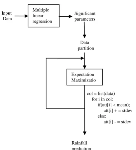
The proposed MLR-EM model is shown diagrammatically in “Fig.1”. The model predicts no rainfall, less rainfall, medium as well as high rainfall. The working of the model is

[image:2.595.310.539.87.339.2]

illustrated in detail.

Fig. 1. MLR-EM model for rainfall prediction

A. The Dataset

For our study we collected five year (2013 to 2017) meteorological data from IMD (Indian Meteorological Department) [8][9]. The parameters of the data includes temp1, temp2 (temperature), hum1, hum2 (humidity), cld1, cld2 (cloud amount), wind1, wind2 (wind), slp1, slp2 (surface pressure) and rainfall. Observed times of the parameters are temp1, hum1, cld1, and wind1 at 7:20 AM. The parameters temp2, hum2, cld2, and wind2 recorded at 2:20 PM. The rainfall and slp1 observed at 8:30 AM, and slp2 at 5:30 PM.

B. Multiple Linear Regression

Multiple linear regression is used for simulating the relation between target variable (z) and multiple explanatory variable (y). The linear equation is given by

0 1 1 2 2

.

n n

z









y





y









y

Where

  

₀

,

₁

,

₂

,..

.



_n are coefficients and

y y

₁

,

₂

,



.

y

_n

are explanatory variable and z denotes estimated variable. The input data has 1826 instances with parameters temp1, temp2, hum1, hum2, cld1, cld2, wind1, wind2, slp1, slp2 and target variable rainfall. Multiple linear regression function was applied on the data set to obtain significant variables that cause rainfall.

1. Regression model was created by calling lm() function in R.

2. Estimate gives intercept value and coefficient values such as , ,… of independent variables. Each coefficient has p-value. The p-value less than 0.05 were considered as influential parameter for

predicting target

variable rainfall.

Input Data

Multiple linear regression

Significant parameters

Data partition

Expectation Maximizatio n

col = list(data) for i in col:

if(att[i] < mean); att[i] + = stdev else:

att[i] - = stdev

(3)

3. Out of ten independent variables hum1, hum2, cld1, wind1 and slp2 were selected as significant and these variables are used to calculate regression equation. 4. In the next step, Expectation Maximization clustering

algorithm was applied on the selected residuals to predict rainfall.

C. Expectation Maximization

Expectation Maximization (EM) is an extension of K-Means clustering algorithm. EM is probabilistic clustering method.

E-step: Expectation step assigns probabilities. Algorithm computes probability for each data point P(b|xi) and assign the points to the clusters.

M-step: Maximization step corresponds to centroid recalculation. Once the data points are assigned to clusters based on the probability, those points will be used to estimate the means and variance to fit the points to a given cluster.

The most significant residuals from multiple linear regression were considered as input to EM algorithm.

The data consist of 1826 records with six variables hum1, hum2, cld1, wind1, slp2 and target variable rainfall. EM algorithm was applied recursively on partitioned data and cluster results were observed. The data partition method was explained step by step and pictorial representation is shown in the “Fig. 2”. The experiment was done on raw data, 0 to 1 normalized data and -1 to 1 normalized data.

1. In the first step 1826 observations were considered, zero rainfall values were assigned to No class and nonzero values were assigned to Yes class. EM algorithm was applied on raw data, 0 to 1 normalized data and -1 to 1 normalized data.

2. In the second step, rainfall = Yes instances were chosen, out of 1826 records 400 records belongs to Yes class. Data from Yes class is divided into Yes-Low and Yes-High. Rainfall value from 0.2mm (minimum) to 50mm ((minimum+maximum/2)) was grouped under Yes-Low and 50.8mm ((minimum+maximum)/2+1) to 100.8mm (maximum) were grouped under Yes-High. 380 instances belong to Yes-Low and 20 instances belong to Yes-High. The instances present in Yes-Low category were classified as Low and High. First 66% of 0.2 to 50 rainfall values were classified as Low and remaining 33% of records were classified as High. EM algorithm was applied on raw data, 0 to 1 and -1 to 1 normalized data.

3. In third step, 20 instances belonging to Yes-High category, were again classified as Low and High. First 33% of 50.8 ((minimum+maximum)/2+1) to 100.8 (maximum) rainfall values were classified as Low and remaining 66% of records were classified as High. EM algorithm was applied on raw data, 0 to 1 and -1 to 1 normalized data.

4. Probabilistic description of each cluster was given by standard deviation and mean. Each column in the data set has mean and standard deviation. Based on cluster results each value of attribute was compared with its mean value, if attribute value is less than mean then add attribute value with standard deviation otherwise subtract with standard deviation. New data set obtained from this procedure was called Yes-Low-stdev and Yes-High-stdev. The same procedure was applied to 0 to 1 and -1 to 1 normalized data. EM algorithm was experimented

[image:3.595.311.515.64.214.2]

on new data set. Correctly and incorrectly classified instances were analyzed.

Fig. 2. Pictorial representation of data partition

IV. EXPERIMENTALRESULTS

Regression model was built by using lm() function in R language. Expectation Maximization algorithm was analyzed using WEKA by selecting classes to cluster evaluation as cluster mode.

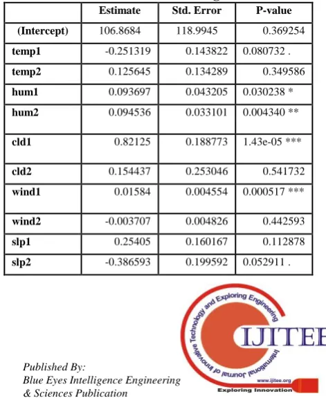
Table I illustrates the results of regression on the data set, the attributes with P-value less than 0.05 are considered significant towards estimated rainfall model. The parameter hum1 has one asterisk means the P-value 0.030238 is less than 0.05, the P-value of hum2 has two asterisk means the value 0.004340 is less than 0.01, cld1 and wind1 has three asterisk means the P-value 1.43e-05 and 0.000517 is less than 0.001. Two and three asterisk indicates that these variables are significant at 99% confidence level, based on these estimation lastly hum1, hum2, cld1, wind1 and slp2 were taken as significant variables for further processing. Mathematical statement of regression was drafted as

Estimated rainfall = 106.868398 + 0.093697 * hum1 + 0.094536 * hum2 + 0.821250 * cld1 + 0.015840 * wind1 - 0.386593 *slp2

The Results of EM algorithm on the data set are shown in the Table II, III, IV, V, VI and VII.

Table- I: Coefficient values for regression model

Estimate Std. Error P-value

(Intercept) 106.8684 118.9945 0.369254

temp1 -0.251319 0.143822 0.080732 .

temp2 0.125645 0.134289 0.349586

hum1 0.093697 0.043205 0.030238 *

hum2 0.094536 0.033101 0.004340 **

cld1 0.82125 0.188773 1.43e-05 ***

cld2 0.154437 0.253046 0.541732

wind1 0.01584 0.004554 0.000517 ***

wind2 -0.003707 0.004826 0.442593

slp1 0.25405 0.160167 0.112878

[image:3.595.312.548.546.834.2]

(4)

*significant, ** more significant, *** most significant parameter.

Table- II: Cluster results of original data

Yes No

Raw data Yes 257 72

correctly clustered instances = 59.1%

No 468 526

Incorrectly clustered instances = 40.8%

Yes No

0 to 1 normalized data

Yes 175 11

No 410 589

Yes No

-1 to 1 normalized data

Yes 175 11

No 410 589

[image:4.595.319.535.74.335.2]

Table- III: Cluster results of Yes class

Low High

Raw data Low 82 73

correctly clustered instances = 50%

High 35 26

Incorrectly clustered instances = 50%

Low High

Low 82 73

High 35 26

Low High

Low 82 73

High 35 26

[image:4.595.65.275.92.293.2]

Table II shows the cluster results of original data explained in step1. Among 1826 observations 1323 observations forms two clusters categorized as Yes and No and remaining instances were treated as noise. Out of 1323 records correctly clustered instances for raw data are 59.1% and incorrectly clustered instances are 40.8%. For 0 to 1 and -1 to 1 normalized data, out of 1826 observations 1185 observations forms Yes and No clusters, correctly clustered instances are 64.4% and incorrectly clustered instances are 35.5%. Data normalization improves clustering results compare to raw data.

Table III describes the result of data set belongs to Yes class. Out of 1826 observations 400 observations belongs to Yes class, from 400 instances 216 instances forms two clusters Low and High. Correctly clustered instances and incorrectly clustered instances are equal to 50% for raw data as well as 0 to 1 and -1 to 1 normalized data. The result was 50% because 0 to (min+max)/2 rainfall values were classified as Low and remaining records were classified as High.

Table- IV: Cluster results of Yes-Low class

Low Hig h

Hig h

6 4

Low Hig h

Low 108 92

Hig h

5 4

Low Hig h

Low 108 92

Hig h

5 4

[image:4.595.61.276.312.540.2]

Table- V: Cluster results of Yes-High class

Low

Raw data Low 13

Hig h

7

Low

Low 13

Hig h

7

Low

Low 13

Hig h

7

As tabulated in Table IV, 380 instances comes under Yes-Low group and 248 instances forms two clusters Low and High in case of raw data and gives out put 60.4% for correctly clustered instances and 39.5% for incorrectly clustered instances. 209 instances forms two clusters Low and High with 0 to 1 as well as -1 to 1 normalized data gives an outcome of 53.58% for correctly clustered instances and 46.4% for incorrectly clustered instances.

[image:4.595.332.521.365.576.2]

(5)

[image:5.595.63.276.66.331.2]

Table- VI: Cluster results of Yes-Low-stdev

Low Hig h

Hig h

5 5

Low Hig h

Low 159 36

Hig h

6 3

Low Hig h

Low 159 36

Hig h

6 3

[image:5.595.318.536.154.645.2]

Table- VII:cluster results of Yes-High-stdev

Low

Raw data Low

13

Hig h

7

Low

Low 13

Hig h

7

Low

Low 13

Hig h

7

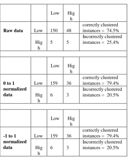
Table VI illustrates the results of dataset Yes-Low-stdev. It has 380 instances and forms two clusters called Low and High with 208 instances. Raw data gives the result of 74.5% for correctly clustered instances and 25.4% for incorrectly clustered instances. As shown in Table IV EM algorithm produces 60.4% of correct cluster instances, when standard deviation value was added or subtracted to each attribute in the raw data and EM algorithm produces correct cluster instances of 74.5%, the result shows correctly clustered instances increased by 14.1%. The same data normalized to 0 to 1 and -1 to 1 and added with standard deviation value forms two clusters Low and High with 204 records. EM algorithm gives 79.4% of correct clustered patterns, as compared to results of normalized data shown in Table IV there is an increment of 25.82% in the cluster outcome. The result shows that error is minimized by adding standard deviation value intern increases the percentage of correct clustered instances

and decreases incorrect clustered instances.

Table VII describes the results of Yes-High-stdev instances appended with standard deviation values. The values of correctly clustered instances are 65% and incorrect instances are 35%. Even though standard deviation value was added, the result remains same. There is no variation in the results because of less number of patterns present in the group.

Table- VIII: Comparison of cluster instances

Fig. 3. Graphical representation of Cluster Instances As shown in Table II, since cluster results of raw data is 59.1% and normalized data is 64.4% our objective to prove rainfall=no becomes true. The result of data set Yes-Low-stdev was 74.5% for raw data and 79.4% for normalized data, our assumption to prove rainfall=less becomes true. By combining the High instances of Yes-Low-stdev and Low instances of Yes-High-stdev, we will get rainfall=medium instances.

Correctly Clustered Instances

Incorrectly Clustered Instances Original Dataset

Raw data 59.10% 40.80% 0 to1 normalized data 64.40% 35.50% -1 to1 normalized data 64.40% 35.50%

Raw-Yes

Raw data 50% 50%

0 to1 normalized data 50% 50% -1 to1 normalized data 50% 50%

Yes-Low

Yes-Low-stdev

Yes-High

Raw data 65% 35%

0 to1 normalized data 65% 35% -1 to1 normalized data 65% 35%

Yes-High-stdev

Raw data 65% 35%

[image:5.595.76.261.354.565.2]

(6)

The cluster result of Yes-High-stdev was about 65%, our intention to prove rainfall=high becomes true. Finally the model was able to predict rainfall=no, less, medium and high, also data normalization gives better cluster results.

Table VIII shows the value of correct and incorrect cluster instances of partitioned data set. Graphical representation of cluster instances is shown in “Fig. 3”. Blue line shows correct cluster instances and brown line shows incorrect cluster instances. After adding standard deviation with the data set the percentage of correct clusters was increased by 74 to 80% in case of Yes-Low-stdev. Cluster results remain same in Yes-High and Yes-High-stdev because the dataset has less number of records. Finally result shows adding or subtracting standard deviation value with the partitioned dataset and also data normalization improves cluster results.

V. CONCLUSION

This work mainly focused on analyzing the various patterns of past meteorological observations. Combination of two methodologies MLR and EM was proposed in the work. MLR predicts humidity, cloud, wind and surface pressure as strong evident parameters for the occurrence of rainfall based on p-value. Partitioned procedure will be applied on selected attributes and EM clustering algorithm was then executed on partitioned data set to determine less, medium and high rainfall. Error correction using standard deviation was used as a measure for errors, which produces 74.5% and 80% of correctly clustered instances and works better for rainfall prediction. Normalization used as a preprocessing enhances the performance of clustering and provides best result.

REFERENCES

1. Asit Subudhi, Manasa Dash, Sukanta Sabut, “Automated segmentation and classification of brain stroke using expectation-maximization and random forest classifier,” Elsevier, Biocybernetics and BioMedical Engineering, 350 (1–13), 2018. 2. Carl-Magnus Svensson, Karen Grace Bondoc, Georg Pohnert, Marc

Thilo Figge, “Segmentation of clusters by template rotation expectation Maximization,” Elsevier, Computer Vision and Image Understanding, (2016) 1–9.

3. Samah M. Alzanin, Aqil M. Azmi, “Rumor detection in Arabic tweets using semi-supervised and unsupervised expectation–maximization,”

Elsevier,Knowledge-Based Systems, 2019.

4. Sihang Qiu, Bin Chen, Rongxiao Wang, Zhengqiu Zhu, Yuan Wang, Xiaogang Qiu, “Atmospheric dispersion prediction and source estimation of hazardous gas using artiﬁcial neural network, particle swarm optimization and expectation maximization,” Elsevier,

Atmospheric Environment, 178 (2018) 158–163.

5. Kaifeng Zhao, Heng Lian, “The Expectation–Maximization approach for Bayesian quantile regression,” Elsevier,Computational Statistics and Data Analysis, 96 (2016) 1–11

6. Mobin Amoozad-Khalili, Reza Rostamian, Mahdi Esmaeilpour-Troujeni, Armaghan Kosari-Moghaddam, “Economic modeling of mechanized and semi-mechanized rainfed wheat production systems using multiple linear regression model,” Elsevier, Information Processing in Agriculture, 2019.

7. Divia Paul A, Ashraf. S.M, J.Ezhilan, Vijayakumar S, Anuj Kapadiya, “A Milestone in Prediction of the Coronary Artery Dimensions from Multiple Linear Regression Equation,” Indian Heart Journal, IHJ 1612, 2019.

8. http://www.imd.gov.in 9. http://www.uas

bangalore.edu.in/index.php/research/agrometeorology

10. Kart-Leong Lim, Han Wang, Xiaozheng Mou, “Learning Gaussian Mixture Model with a Maximization-Maximization Algorithm for Image Classiﬁcation,” 12th IEEE International Conference on Control &

Automation (ICCA), Kathmandu, Nepal, June 1-3, 2016.

11. Gemma Morral, Pascal Bianchi, Jeremie Jakubowicz, “On-Line Gossip-Based Distributed Expectation Maximization Algorithm,” 2012 IEEE Statistical Signal Processing Workshop (SSP).

12. Zhenyue Zhang, Yiu-ming Cheung, “On Weight Design of Maximum Weighted Likelihood and an Extended EM Algorithm,” IEEE Transactions on Knowledge and Data Engineering, Vol. 18, No. 10, October 2006.

13. Christian Kern, Thorsten Stefan, Jorg Hinrichs, “Multiple linear regression modeling: Prediction ofcheese curd dry matter during curd treatment,” Elsevier, Food Research International, 2018.11.061. 14. G. Ciulla, A. D Amico, “Building energy performance forecasting: A

multiple linear regression approach,” Elsevier,Applied Energy, 253 (2019) 113500.

15. Harsha S, N Bhaskar, Amith Kumar, V Pujari and Nibha, “A Novel Method to Dig Information from Generic Groups of Enriched Records (DIgGER),” ResearchGate, IJCSSEIT, Vol. 5, No. 2, December 2012, pp. 243-248.

16. Shobha N, Asha T, “Influential parameters on rainfall forecasting using multiple linear regression,” 2019 JETIR February 2019,

Volume 6,Issue 2 (ISSN-2349-5162).

17. Pang-Ning Tan, Michael Steinbach, Vipin Kumar, “Introduction to Data mining,” Pearson Education, 2007.

18. Jiawei Han and Micheline Kamber, “Data Mining Concepts and Techniques”.

AUTHORSPROFILE

Shobha. N working as Assistant Professor in the Department of Information Science & Engineering, APS College of Engineering, Bengaluru. Currently pursuing Ph.D in Computer Science & Engineering at VTU in the area of Data Mining, published 5 papers in International journals and Conferences.

Dr. Asha. T is a Professor & HOD in the Department of Computer Science & Engineering, Bangalore Institute of Technology, Bengaluru. She obtained her Ph.D in Computer and Information Science from Visvesvaraya Technological University, Karnataka. She has published around 31 papers in International/National journals and Conferences.

Her research interests include Data Mining, Medical Informatics, Machine Learning, Pattern Recognition and Big data management etc., email:

[email protected], [email protected]