Estimation for Geostatistical Data
Nelson Jinn-Yih Chua
Supervised by Prof A. H. Welsh and
Dr Francis K. C. Hui
A thesis submitted in partial fulfilment of the requirements for the degree of Bachelor of Statistics with Honours in Statistics
at the Australian National University.
This thesis contains no material which has been accepted for the award of any other degree or diploma
in any University, and, to the best of my knowledge and belief, contains no material published or written
by another person, except where due reference is made in the thesis.
Nelson Jinn-Yih Chua
First and foremost, I would like to express my utmost gratitude for my supervisors Alan and Francis, who
were absolutely pivotal to the development of this thesis. Alan’s wealth of knowledge and experience
ensured that I progressed with a high level of efficiency. Meanwhile, Francis provided extensive
guid-ance on the application of the expanding domain and infill frameworks in both a geostatistical context
and for thesis writing. Francis and I also had enjoyable pseudo-intellectual discussions about
Conver-gence and partial residuals; albeit at the expense of Alan. Their tremendous dedication and passion is
<v e r y g o o d> and much appreciated.
I would also like to thank my friends and family for their continued care and support over the year.
Special thanks goes to Jiabin for enlightening me about the existence of parallel processing inR, without
which I would still be hoping for my simulation to be complete by the end of next year. I would also like
to thank Nickson for peer-reviewing my work throughout the year, as well as for engaging in
Parameter estimation and inference in a geostatistical model is often made challenging due to the strong
dependence between nearby observations. For large sample sizes, maximum likelihood estimation
quickly becomes computationally expensive to perform, so other estimation approaches such as
maxi-mum composite likelihood estimation have been proposed as alternatives. In this thesis, we investigate
the statistical and computational performance of maximum composite likelihood estimation relative to
maximum likelihood estimation for the Gaussian exponential covariance model. As the main
contribu-tion of this work, we derive and analyse the exact closed-form expressions for the sandwich covariance
matrix of various composite likelihoods in one-dimensional space. These new results are found under a
hybrid asymptotic framework, which unifies the traditional expanding domain and infill frameworks seen
in the geostatistical literature. We then demonstrate the practical implementation of maximum
compos-ite likelihood approaches for estimation and inference, as well as perform a data-motivated simulation
Abstract iii
1 Introduction 1
1.1 Geostatistical Framework . . . 2
1.2 Covariance and Variograms . . . 3
1.3 Maximum Likelihood Estimation . . . 5
1.4 Asymptotics of Maximum Likelihood Estimation . . . 6
1.5 Maximum Composite Likelihood Estimation and Asymptotics . . . 8
1.6 Asymptotics in a Geostatistical Framework . . . 10
1.7 Thesis Outline . . . 11
2 Literature Review 13 2.1 Maximum Likelihood Estimation in Geostatistics . . . 14
2.2 Asymptotics for the Gaussian Exponential Covariance Model . . . 17
2.3 Maximum Composite Likelihood Estimation in Geostatistics . . . 19
3 Theory: Gaussian Exponential Covariance Model in One Dimension 24 3.1 Equally-Spaced Lattice Construction . . . 25
3.2 Full Likelihood . . . 26
3.2.1 Derivation of the Inverse Fisher Information Matrix . . . 26
3.2.2 Asymptotics . . . 30
3.3 Composite Conditional 2-Nearest Neighbours Likelihood . . . 32
3.3.1 Construction of the Composite Likelihood . . . 33
3.3.2 Derivation of the Sandwich Covariance Matrix . . . 36
3.3.3 Asymptotics and Relative Efficiency . . . 41
3.4 Composite Marginal Blockwise Likelihood . . . 43
3.4.1 Construction of the Composite Likelihood . . . 44
3.4.2 Derivation of the Sandwich Covariance Matrix . . . 45
4 Data and Simulation: Gaussian Exponential Covariance Model in Two Dimensions 56
4.1 Analysis of Maximum Temperature Dataset . . . 57
4.2 Maximum Composite Likelihood Estimation . . . 59
4.3 Variance Estimation of Maximum Composite Likelihood Estimates . . . 62
4.4 Application to Maximum Temperature Dataset . . . 65
4.5 Simulation Study . . . 70
4.5.1 Model without Nugget Effect . . . 71
4.5.2 Model with Nugget Effect . . . 73
5 Conclusion 76 5.1 Main Contributions . . . 76
5.2 Further Research . . . 78
A Detailed derivation of the trace of a four-matrix product 80
1.1 Region of leeway for a directional semivariogram . . . 4
1.2 Comparison of asymptotic frameworks for geostatistical data . . . 10
3.1 Setup of observation locations on a line for the hybrid asymptotic framework . . . 25
3.2 Asymptotic relative efficiency of the maximum composite conditional 2-nearest
neigh-bours likelihood estimator . . . 42
3.3 Asymptotic relative efficiency of the maximum composite marginal blockwise
likeli-hood estimator . . . 53
3.4 Asymptotic relative efficiency of the maximum composite marginal blockwise
likeli-hood estimator for values ofρ0near 1 . . . 54
4.1 United States mean maximum temperatures in January 2000 atN=1052 locations. . . . 57 4.2 Empirical semivariograms of the mean-normalised maximum temperature data . . . 59
4.3 Example setup of observation order for the composite conditional K-sequential neigh-bours likelihood . . . 60
4.4 Standardised residual diagnostic plots for the maximum temperature spatial regression
model . . . 66
4.5 Maximum composite marginal blockwise likelihood estimation for the maximum
tem-perature spatial regression model . . . 67
4.6 Runtime of various computations for the composite marginal blockwise likelihood . . . 67
4.7 Random subset of locations used for simulations . . . 70
4.8 Empirical relative efficiency of maximum composite marginal blockwise likelihood
es-timation under the exponential covariance model without a nugget effect . . . 71
4.9 Empirical relative efficiency of maximum composite marginal blockwise likelihood
4.1 Estimates and 95% Wald confidence intervals for various choices of composite
condi-tional likelihood compared to the full likelihood. . . 68
4.2 Runtime of various computations for the composite conditional K-nearest neighbours likelihood compared to the full likelihood . . . 69
4.3 Empirical relative efficiency of for various choices of composite conditional likelihood
under the exponential covariance model without a nugget effect . . . 72
4.4 Empirical coverage probabilities of the Wald confidence interval for various choices of
composite likelihood under the exponential covariance model without a nugget effect . . 73
4.5 Empirical bias and proportion of zero estimates for various choices of composite
likeli-hood under the exponential covariance model with a nugget effect . . . 73
4.6 Empirical relative efficiency for various choices of composite conditional likelihood
un-der the exponential covariance model with a nugget effect . . . 74
4.7 Empirical coverage probabilities of the Wald confidence interval for various choices of
Introduction
Spatial data consists of observations that are collected over a geographical area. Such data are common
in a wide variety of disciplines including ecology (Fortin et al., 2012), climatology (Nowak et al., 2017),
demography (Matthews and Parker, 2013) and geology (Angelini and Heuvelink, 2018). The rise of the
information age has seen a sharp increase in the amount of spatial data being collected; and what comes
with it is a greater demand for analytical tools and methodologies to understand the data. Due to the size
and complexity of these datasets, it is also important to consider methods of analysis and inference that
are computationally efficient.
There are three main categories that spatial data fall under: geostatistical, areal (or lattice) and point
process data (Cressie and Wikle, 2011, p. 124). Geostatistical data is where the variables of interest
are observed at fixed collection points. On the other hand, areal data are concerned with variables that
are aggregated over well-defined geographical areas, such as cities and territories. The implication of
this in terms of asymptotics is that in a geostatistical setting, we are free to obtain more observations at
different locations in our spatial domain, but for areal data, further observations are only possible as part
of a longitudinal study; that is, through the introduction of a temporal dimension. Finally, point process
data occur when the locations at which observations occur are random and may themselves be of interest.
The methods and models used to analyse each of these types of spatial data are quite different, and we
will focus our attention towards geostatistical data for this thesis. Our motivating data for this will be
maximum temperature data of the United States, which has been recorded at over one thousand land
1.1
Geostatistical Framework
Consider observing a variable of interestz at a set of locations {s1,s2, ...,sN}, wheresi∈
S
⊆Rd for d∈Z+. It is common in the literature to assume that these observations are subject to random additivemeasurement errorsε(si)(Cressie and Wikle, 2011, p. 121). Thus,zcan be related to the true unobserved spatial processyaccording to the following:
z(si) =y(si) +ε(si).
By imposing specific distributional assumptions on the processes{y(s)}and{ε(s)}, this becomes a para-metric geostatistical model. In particular, this thesis will focus on the case where{y(s)}is a Gaussian process, as defined below, andε(s) are independent and identically distributed (i.i.d.) normal random
variables with zero mean and varianceτ2, whereτ2 is known as the nugget effect (Cressie and Wikle,
2011, p. 121). By extension, due to the additive property of Gaussian random variables, this means that
{z(s)}is also a Gaussian process.
Definition 1.1(Gaussian process) A process{w(s):s∈
S
⊆Rd}is Gaussian if its finite dimensional distributions are Gaussian; that is, for any finite subset of locations{s1,s2, ...,sn} ⊂S
, we have thatthe random vector(w(s1),w(s2), ...,w(sn))T∼N(µ,Σ)for some mean vectorµ∈Rnand covariance matrixΣ∈Rn×n.
A key feature of spatial data is the strong dependence between nearby observations. As per Tobler’s first
law of geography, “Everything is related to everything else, but near things are more related than distant
things.” (Tobler, 1970) Hence, it is important to account for spatial correlation when analysing spatial
1.2
Covariance and Variograms
A common simplifying assumption to make about a spatial process is for it to be (weakly) stationary
(Cressie and Wikle, 2011, p. 129).
Definition 1.2(Stationary spatial process) A spatial process{z(s):s∈
S
⊆Rd}is (weakly) station-ary ifE[z(s)]≡µz, var[z(s)]<∞and cov[z(s),z(s+h)] =E[(z(s)−µz)(z(s+h)−µz)]≡Cz(h)for alls,s+h∈S
.Under the assumption of stationarity, the strength of dependence between observations, as expressed
through the covariance, is only dependent on their distance and direction apart. This acts as a kind of
smoothness which aids in the interpretability of a parametric model by reducing the number of
parame-ters needed to describe a system. It is often used when the behaviour of the response variable is thought
to be roughly homogeneous over the spaceS. If, further to this, it is believed that the dependence decays in a radial manner from each location, then an additional restriction of covariance depending only on the
some metrick · k(such as Euclidean distance) can be imposed:
Definition 1.3(Isotropic covariance) A covariance structure is isotropic if cov[z(s),z(s+h)]≡
Cz(khk)for alls,s+h∈
S
.In the time series literature, a common tool used to select an appropriate model for the covariance
structure is the autocorrelation function, which estimates the covariance between observations at each
time difference. However, due to the often multidimensional nature of
S
and the presence of a nuggeteffect, it is common to use a variogram instead when analysing geostatistical data (Gneiting et al., 2001).
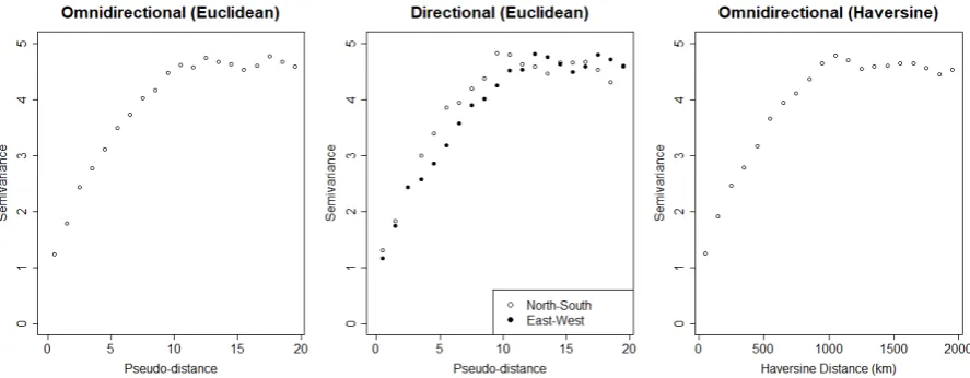
Definition 1.4(Variogram) The variogram for a stationary covariance structure is calculated by 2γz(h)≡var[z(s)−z(s+h)] =2(Cz(0)−Cz(h)). The quantityγz(h)is known as the semivariogram.
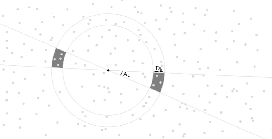
Figure 1.1: Region of leeway for a directional semivariogram. For alli, we identify the observations indexed by
j>ithat lie in the tolerance regionTbc(filled dark grey regions).
the mean squared difference ofzfor all pairs of observations that arekhkunits apart, with a degree of leeway. If, in addition, the leeway is further partitioned by direction, as illustrated in Figure 1.1, this
is known as a directional semivariogram. This is typically used to assess the validity of assuming an
isotropic covariance structure.
Definition 1.5(Empirical semivariogram for two-dimensional space) Let
S
∈R2 and consider a set of partitions with distance cut-offs 0=d0 <d1 < ... <dmax and angle cut-offs −π/2−δ= a0<a1 < ... <amax =π/2−δ with 0≤δ<π. Let the separation vector be denoted as hi j = si−sj = (hi j,1,hi j,2)T for all 1≤i< j≤N. For each pair of intervals (Db,Ac), where Db =(db,db+1],A0= (π/2−δ,π/2]∪(−π/2,a1]andAc= (ac,ac+1]forc=6 0, letTbc={(i,j):||hi j|| ∈
Db,arctan(hi j,2/hi j,1)∈Ac}be the region of leeway. Then the empirical semivariogram for the mid-point ofDbandAcis given by
ˆ
γz(Db,Ac)≡ 1
2|Tbc|(i,
∑
j)∈T bc(z(si)−z(sj))2,
The shape of an empirical semivariogram with respect to distance is then assessed in order to determine
an appropriate parametric model. Commonly used isotropic covariance structures include the spherical
and Mat´ern; the latter of which encompasses the exponential and squared exponential as special cases
(Stein, 1999, p. 31). For this thesis, we will focus on the exponential covariance structure as it is one of
the simplest and widely explored cases in the literature (Gneiting et al., 2001).
Definition 1.6(Exponential covariance) A mean-stationary spatial processz(s)has an exponential covariance structure ifCz(h) =τ2I(khk=0) +σ2exp(−αh), or equivalently, γz(h) =τ2I(khk 6= 0) +σ2(1−exp(−αh)), whereI(·)is the indicator function.
Under this particular covariance structure, the covariance matrixΣcan be manipulated algebraically in
certain basic geostatistical settings, such as having closed-form expressions for the inverse and
determi-nant (Kac et al., 1953).
1.3
Maximum Likelihood Estimation
Once a parametric spatial model has been specified for the dataz= (z(s1),z(s2), ...,z(sN))T, with un-known true parameter values stored in the vectorθ0∈Θ⊆Rp for p∈Z+ and p≤n, it is of interest to estimate and perform inference onθ. One widely used starting point for this is maximum likelihood estimation, where an estimate ˆθis chosen such that it maximises the likelihood of obtaining the observed data.
Definition 1.7(Maximum likelihood estimate) The maximum likelihood estimate ofθ0under a spec-ified model forzwith joint density f(z;θ)≡
L
(θ;z)is ˆθML=argmaxθ∈Θ
L
(θ;z). Equivalently, one can maximise the log-likelihood function; that is, ˆθML=argmax
θ∈Θ
`(θ;z)≡argmax
θ∈Θ
log
L
(θ;z).Such optimisation problems are usually solved by taking the first-order partial derivatives of the objective
the score function sc(θ;z)≡ ∂
∂θ`(θ;z). After solving sc(θ;z) =0, the (observed) information function
info(θ;z)≡ − ∂2
∂θ∂θT`(θ;z)may then be used to determine the nature of the stationary points found. In particular, a stationary point is (at least) a local maximum if the information matrix evaluated at the
stationary point is positive definite.
The following theorem by Bartlett (1953) highlights a useful property of the score function:
Theorem 1.1(Expected score equals zero) Suppose that the interchange of differentiation and inte-gration is permissible atθ0∈Θ. ThenE[sc(θ0;z)] =0.
Proof: E[sc(θ0;z)] =R−∞∞ sc(θ0;z)f(z;θ0)dz=R−∞∞
∂ ∂θ0f(z;θ0)
f(z;θ0) f(z;θ0)dz= ∂ ∂θ0
R∞
−∞f(z;θ0)dz= ∂
∂θ0(1) =0.
This is a necessary condition for the maximum likelihood estimator to be asymptotically unbiased
(Lind-say, 1988).
A quantity associated with the variances and covariances of the estimator ˆθ is the Fisher information matrixI(θ)≡var[sc(θ;z)] =E[sc(θ;z)sc(θ;z)T]. Alternatively, we can use Theorem 1.1 to show that the Fisher information matrix can also be computed usingI(θ) =E[info(θ;z)] (Bartlett, 1953). The Fisher information matrix will be shown to play an important role in the asymptotic properties of the
maximum likelihood estimator in Section 1.4.
1.4
Asymptotics of Maximum Likelihood Estimation
A desirable property of any estimator is consistency, meaning that it will approach the true parameter
valueθ0as more data are collected.
We may alternatively consider the notion of consistency in mean square error, which is a sufficient
condition for consistency (by Chebyshev’s inequality) and usually easier to apply.
Definition 1.9(Consistency in mean square error) An estimator ˜θis consistent in mean square error if the mean square error mse[θ˜]≡E[(θ˜−θ0)2] ={bias[θ˜]}2+var[θ˜]satisfies limN→∞mse[θ˜] =0. It is also desirable for an estimator to have low variability. Cram´er (1946, p. 477-481) and Rao (1945),
amongst other statisticians around the same time, derived the theoretical lowest variance attainable by
an unbiased estimator.
Theorem 1.2(Cram´er-Rao lower bound) Suppose that ˜θ is an unbiased estimator for θ0. Then var[θ˜]≥I(θ0)−1.
Note that the above theorem holds regardless of the dependence structure of the data. However, in the
classical scenario in which asymptotics of the maximum likelihood estimator were established, the data
are assumed to be independent and identically distributed. The following theorem highlights the key
asymptotic result in this context; it is presented in many statistical inference textbooks such as Casella
and Berger (2002).
Theorem 1.3(Maximum likelihood asymptotics for i.i.d. data) Letz1,z2, ...,zN iid
∼ f(z;θ0), where f satisfies various regularity conditions (including differentiability with respect toθ and parame-ter identifiability; see Casella and Berger (2002, p. 516) for further details). Then the maximum
likelihood estimator follows an asymptotically normal distribution; that is, ˆθML ·
∼N(θ0,I(θ0)−1). This theorem implies that the maximum likelihood estimator is consistent and asymptotically achieves
1.5
Maximum Composite Likelihood Estimation and Asymptotics
Maximum composite likelihood estimation involves deliberately using a misspecified but structurally
simpler likelihood as the objective function to be maximised, in place of the full likelihood
L
(θ;z). The motivation behind using this estimation approach for geostatistical models is due to the complicationsassociated with a strong dependence structure. The full likelihood may be difficult to write down
explic-itly; or even if we can, maximising this function may be computationally intractable. As an example,
in the case of a Gaussian process, evaluating the full likelihood relies on finding the determinant and
inverse of the N×N covariance matrix Σ, both of which have computational costs of
O
(N3) in the absence of any exploitable matrix structure. This is problematic from a computational standpoint if thenumber of observations in the dataset to be analysed is large.
Varin et al. (2011) classify composite likelihoods into two broad categories, which describe whether the
likelihood is composed of marginal or conditional densities, respectively:
Definition 1.10(Types of composite likelihood) Let
B
kcorrespond to some subset of the observations{z(s1), ...,z(sN)}. A composite likelihood
L
C(θ;z)is called marginal if it is of the formL
C(θ;z) = ∏Bb=1f(B
b;θ),and conditional if it is of the formL
C(θ;z) =∏Ni=1f(y(si)|B
i;θ).Once a composite likelihood has been constructed, the maximum composite likelihood estimator ˆθCL can be found in a similar manner to maximum likelihood estimation. Firstly, we can find
station-ary points of the composite log-likelihood c`(θ;z) ≡log
L
C(θ;z) using the composite score func-tion scC(θ;z)≡ ∂∂θc`(θ;z). We can then identify maxima using the composite information function infoC(θ;z)≡ −∂θ∂TscC(θ;z).
The asymptotics of maximum composite likelihood estimation differ slightly from maximum likelihood
estimation. Firstly, we note that composite likelihood functions are almost always constructed to satisfy
proof to Theorem 1.1:
Theorem 1.4(Expected composite score equals zero) Suppose that the interchange of differentia-tion and integradifferentia-tion is permissible atθ0. ThenE[scC(θ0;z)] =0, where the expectation is taken with respect to the true likelihood of the data f(z;θ0).
Proof:Note that the conditional densities f(z(si)|
B
i;θ)that comprise a composite conditional like-lihood can be expressed as the ratio of two marginal densities. Hence, both the composite marginallog-likelihood and a composite conditional log-likelihood can be written as a linear combination of
marginal log-densities; that is,c`(θ;z) =∑bmblogf(
B
b;θ), with coefficientsmb∈ {−1,1}. Thus, E[scC(θ0;z)] =∑bE[∂
∂θ0f(Bb;θ0)
f(Bb;θ0) ] =∑b
R∞
−∞∂∂θ0f(
B
b;θ0)dB
b=0.However, the asymptotic variance of maximum composite likelihood estimation is a quantityG(θ)−1
known as the sandwich covariance matrix, which takes the place of the inverse Fisher information
I(θ)−1. This is highlighted in the following theorem available from Kent (1982) and Lindsay (1988): Theorem 1.5(Maximum composite likelihood asymptotics for i.i.d. data) Letz1, ...,zN
iid
∼ f(z;θ0), where the densities comprising the composite likelihood satisfy the regularity conditions from
The-orem 1.3. DefineJ(θ)≡var[scC(θ;z)] =E[scC(θ;z)scC(θ;z)T]andH(θ)≡E[infoC(θ;z)], which comprise the sandwich information matrixG(θ)≡H(θ)J(θ)−1H(θ). Then the asymptotic distribu-tion of the maximum composite likelihood estimator is given by ˆθCL
·
∼N(θ0,G(θ0)−1).
Note that in the case of the full (correctly specified) likelihood function, we have thatH(θ) =J(θ) =
I(θ), which collapses down to maximum likelihood estimation and Theorem 1.3.
It is important to note that the use of the structurally simpler composite likelihood over the full likelihood
involves a trade-off between computational efficiency and statistical efficiency. In particular, it is often
the case thatI(θ)−G(θ)is a positive semi-definite matrix (Varin, 2008), so there is less information from the data being utilised in estimatingθ0using ˆθCLthan ˆθML. Thus, we would like to investigate the extent of information loss from various choices of composite likelihood, and will be the focus of this
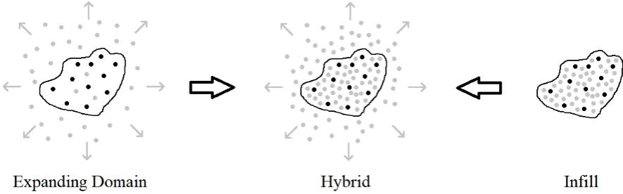
Figure 1.2: Comparison of asymptotic frameworks for geostatistical data. The black-bordered region and points denote the initial region of collection and locations of observations; grey points are further observation locations under the corresponding asymptotic framework.
of the elements inI(θ)−1to the corresponding elements inG(θ)−1.
1.6
Asymptotics in a Geostatistical Framework
The classical asymptotic results for maximum likelihood estimation and maximum composite likelihood
estimation, as highlighted in Theorems 1.3 and 1.5, rely on the assumption that the data are independent
and identically distributed. However, since this does not hold in the context of geostatistical models,
there is no guarantee that the favourable asymptotic properties of these two approaches still hold.
Addi-tionally, as illustrated in Figure 1.2, there are generally three different asymptotic frameworks that can
be considered for geostatistical data: expanding domain, infill and hybrid.
Expanding domain asymptotics assume that observations continue to be taken over an increasing region
of space out to infinity. This can be likened to taking future observations in a time series, where time is
treated as a uni-directional one-dimensional space. Infill asymptotics, on the other hand, focus on taking
an increasing density of observations within a closed region. It is often the case in spatial data that the
geographical region of interest is closed, so analysis of infill asymptotics is desired.
By combining the notions of expanding domain and infill together, a third framework called hybrid
of the favourable asymptotic properties of the expanding domain framework (see Section 2.1) and use
them in an infill context, including spatial prediction. This has applications in contexts where we can
increase both the spatial resolution and domain of our observations, such as demographic studies (Lu
and Tjøstheim, 2014).
Although hybrid asymptotics have been considered in papers as early as Hall and Patil (1994) and Lahiri
et al. (2002), the framework has largely been overlooked until more recently. A unifying formalisation
of all three asymptotic frameworks is presented in Lu and Tjøstheim (2014), where they define∆j,N≡
max{||si−sj||: 1≤i≤N,i6= j}andδj,N ≡min{||si−sj||: 1≤i≤N,i6= j}, which correspond to the maximum and minimum distance betweensj and the other locations in the set of sizeN, respectively. These quantities are used in the following definition:
Definition 1.11(Asymptotic frameworks) Consider a sequence of subsets of locationsS1,S2, ...,SN⊂
S
, whereSjhasjlocations and the sequence is not necessarily nested. Then the following conditionsdefine the corresponding asymptotic frameworks:
• Expanding domain:∆N≡ min
1≤j≤N∆j,N→∞asN→∞and limN→∞1min≤i≤Nδi,N≥L>0
• Infill: δN≡ max
1≤j≤Nδj,N→0 asN→∞and limN→∞1max≤i≤N∆i,N ≤U<∞
• Hybrid:∆N →∞andδN→0
In this thesis, the sequence of sampling locations will be structured in a way that will allow for analysis
of spatial models under the hybrid framework. This will also allow for analysis under the expanding
domain and infill frameworks.
1.7
Thesis Outline
The primary objective of this thesis is to compare the statistical and computational performance of
maximum composite likelihood estimation relative to maximum likelihood estimation in a geostatistical
maximum likelihood estimation, but it is important to discern whether using a misspecified likelihood is
a viable alternative when the sample size is large and using the full likelihood is no longer feasible.
In Chapter 2, we shall review the literature on maximum likelihood and maximum composite likelihood
estimation in a Gaussian geostatistical setting. In particular, we are interested in the asymptotic
frame-works from Definition 1.11 where asymptotic normality of these estimators is shown to still hold even
without the i.i.d. data assumption. We will then narrow our focus to results for maximum likelihood
estimation under a Gaussian exponential covariance model, which has been widely studied in the
litera-ture. We will also highlight some choices of composite likelihood that have been studied, which reveals
the lack of theoretical asymptotic results in the literature.
As the main contribution of this thesis, in Chapter 3, we explore the theoretical asymptotic efficiency
of two choices of composite likelihood relative to the full likelihood in a one-dimensional exponential
covariance model. We derive exact closed-form expressions for the sandwich covariance matrixG(θ)−1
for these two choices and compare this to the inverse Fisher informationI(θ)−1to obtain the asymptotic
relative efficiency of these maximum composite likelihood estimators. This leads to new insights that
would have been difficult to uncover from a simulation study alone, such as the effect of the strength of
spatial correlation on efficiency.
In Chapter 4, we look at the practical implementation of composite likelihoods in the context of
mod-elling maximum temperature data for the United States. This will involve the derivation of a broadly
applicable variance estimator for maximum composite likelihood estimates in a Gaussian setting. We
will use this example to motivate a simulation study in the two-dimensional exponential covariance
setting, and draw comparisons with our findings in Chapter 3.
Finally, we will summarise our findings and contributions in Chapter 5. We will also identify potential
Literature Review
Classical asymptotics to do with maximum likelihood and maximum composite likelihood estimation
are derived under the assumption that the data are independent and identically distributed. Hence, in
Section 2.1 of this literature review, we will highlight some of the asymptotic results available for
max-imum likelihood estimators in a geostatistical setting. In particular, we are interested in the conditions
that are sufficient for consistency and asymptotic normality to still hold. Close attention will be paid to
the asymptotic framework that is being considered, and how it is compatible with Definition 1.11.
Next, in Section 2.2, we will review the results that are available for maximum likelihood estimation
asymptotics under a Gaussian exponential covariance model. This will cover many different cases, such
as the dimension of space and whether or not a nugget effect is included. We will check that these results
are consistent with the general theory in Section 2.1. The findings here will also allow us to set up a
reliable benchmark when comparing maximum composite likelihood estimation to maximum likelihood
estimation.
In Section 2.3, we will highlight the various choices of composite likelihood that have been
previ-ously studied in the geostatistical literature. For each type of composite likelihood, we will look at the
motivation behind its construction, as well as any theoretical or numerical studies of their statistical
per-formance. A few of these composite likelihood functions will be explored in our exponential covariance
2.1
Maximum Likelihood Estimation in Geostatistics
One of the earliest papers dealing with maximum likelihood asymptotics in a geostatistical setting is due
to Mardia and Marshall (1984). Here, they worked in the context of Gaussian spatial regression, where
z= (z(s1),z(s2), ...,z(sN))T∼N(Xβ0,Σ(φ0))for anN×qcovariate matrixXand vector of true param-etersθ0= (βT0,φ0T)T ∈Θ⊆Rq+p. Applying some general results from Sweeting (1980), they identified sufficient conditions for the consistency and asymptotic normality of the maximum likelihood estimator
ˆ
θML. These conditions pertain to the continuity, growth and convergence of the observed information
function info(θ;z)≡ − ∂2
∂θ∂θT`(θ;z)and Fisher informationI(θ)≡var[sc(θ;z)] =E[sc(θ;z)sc(θ;z)
T].
Theorem 2.1(Maximum likelihood asymptotics for spatial regression) Suppose that the usual reg-ularity conditions from Theorem 1.3 hold, in addition to the covariance function having continuous
second-order partial derivatives with respect toφ. Furthermore, assume limN→∞I(θ)−1=0 and that
−I(θ)−12info(θ)I(θ)− 1
2 converges in probability to the identity matrix. Then ˆθML∼· N(θ0,I(θ0)−1) with a convergence rate of√N.
In practice, Theorem 2.1 is often difficult to verify, so Mardia and Marshall (1984) then considered
sufficient conditions for asymptotic normality to hold under the expanding domain framework.
Theorem 2.2(Maximum likelihood expanding domain asymptotics) Let z have a stationary co-variance structureCz(h), and{s1,s2, ...,sN} form an equally-spaced regular lattice on Rd. Define
H
N ≡ {si−sj;i,j∈ {1,2, ...,N}} to be a set containing all of the unique displacements betweenany two observations on the lattice. Suppose that limN→∞(XTX)−1=0and the parameters inφare not asymptotically linearly dependent. If limN→∞∑h∈HN|Cz(h)|<∞, limN→∞∑h∈HN|∂φ∂kCz(h)|<∞ and limN→∞∑h∈HN| ∂
2
∂φk∂φlCz(h)|<∞for allk,l=1,2, ...,p, then we have that ˆθML ·
∼N(θ0,I(θ0)−1) with a convergence rate of√N.
The above theorem is only applicable in the expanding domain framework due to the requirement for the
enough information about the covariance parametersφavailable in the data, and this is reliant on having some observations that are far enough apart such that they are effectively uncorrelated. Due to the
nature of an expanding domain, as the sample sizeNincreases, displacementshthat are progressively introduced to the set
H
N will get larger in magnitude, and thus contribute comparably less to thesesums. In contrast, under the infill framework, new displacements that are added to
H
N will be near0,causing the sums to diverge. This suggests that observations that are close to each other are too strongly
correlated and hence provide less information aboutφ, which in turn demonstrates that the asymptotic behaviour of the maximum likelihood estimator under different asymptotic frameworks can vary.
A consequence of Theorem 2.2 is that ifφinvolves a nugget effect termτ2, then asymptotic normality ofθholds if and only if it would otherwise hold in the absence of the nugget effect; that is, for the latent spatial processy. Since the nugget effect only appears as an additive term in the covariance function at a
displacement of0, we have that∑h∈HN|Cz(h)|=τ2+∑h∈HN|Cy(h)|and∑h∈HN|∂τ∂2Cz(h)|=1, with no other differences between the sums forzandy.
In the context of a spatial autoregressive model, Zheng and Zhu (2012) obtained general results for
maximum likelihood asymptotics under the expanding domain, infill and hybrid frameworks. This
ex-tends on the results of Lee (2004) who considered the expanding domain framework alone. The spatial
autoregressive model is given byz=Xβ0+, where the errors are modelled using the autoregressive structure=WN(φ0)+ν, and the weighting matrixWN(φ) = (wi j,N)N×N has a diagonal of zeroes andνi
iid
∼N(0,η20).
An essential component of the asymptotic theory by Zheng and Zhu (2012) is the ratemN at which the off-diagonal elements in the weighting matrix decay to zero; that is,wi j,N =
O
(mN−1)fori6= j. Based on this, mN =O
(1) corresponds to expanding domain,mN →∞withmN/N→C>0 corresponds to infill, and mN →∞ with mN/N→0 corresponds to the hybrid framework. As an example, we can consider a common choice for weights which uses distance-based neighbours, where each row sums toconsideration. Under expanding domain, the number of distance-based neighbours will remain finite
so the weights will not decay to zero; but under the infill and the hybrid frameworks, the number of
distance-based neighbours will grow to infinity. However, in the hybrid case, as long as the domain
expands,Nwill grow at a faster rate thanmN, so thatmN/Nwill converge to zero.
Theorem 2.3(Maximum likelihood asymptotics for spatial autoregression) Assume a set of regular-ity conditions related to the boundedness ofWN(φ)andXare satisfied (see Zheng and Zhu (2012) for more details). Then ˆβML and ˆη2MLare consistent and follow an asymptotic normal distribution with a convergence rate of√N. However, the asymptotics for ˆφML differ depending on the asymp-totic framework being considered.
• IfmN=
O
(1)then ˆφML p→φ0. Furthermore, if limN→∞N−1Iφ(θ)exists and is positive
defi-nite, whereIφ(θ)is the block of the Fisher information matrix dealing exclusively with partial
derivatives ofφ, then ˆφML ·
∼N(φ0,Iφ(θ0)−1)with a convergence rate of
√
N.
• IfmN→∞andmN/N→0, then ˆφML p
→φ0. However, the convergence rate ispN/mN.
• IfmN→∞andmN/N→C>0, then the consistency of ˆφMLis not guaranteed.
Both Theorems 2.2 and 2.3 validate the idea that the usual asymptotics of maximum likelihood
estima-tion can be translated to an expanding domain setting. We also see from Theorem 2.3 that asymptotic
normality holds under a hybrid framework simply due the domain being able to expand. However, the
asymptotics of maximum likelihood estimation for covariance parameters under the infill framework can
be problematic. Once again, this highlights the idea that there is too little information about the strength
of dependence between observations when the domain is fixed, even as the sample size increases.
Due to the favourable asymptotic behaviour of estimators under the expanding domain framework, most
results in the geostatistical literature are derived in this setting. Meanwhile, infill is often only considered
in specific cases such as the Gaussian exponential covariance model that will be discussed in Section
2.2. Finally, due to the lack of formalisation of the hybrid framework until more recently in Zheng and
2.2
Asymptotics for the Gaussian Exponential Covariance Model
As one of the most widely studied geostatistical models, we will now review some results for maximum
likelihood estimation asymptotics under a Gaussian exponential covariance model, as per Definition
1.6. Given results such as Theorems 2.1 and 2.3, most of the interest in geostatistical asymptotics lies in
the specified covariance structure rather than linear regression component, so this section will focus on
zero-mean exponential covariance models.
In a one-dimensional setting on an equally-spaced lattice, Zhang and Zimmerman (2005) considered the
expanding domain asymptotics of the Gaussian exponential covariance model. For this they used the
observation locationssi=i, and model (z(s0),z(s1), ...,z(sN))T ∼N(0,Σ0)with true parameter vector
φ0= (σ20,α0,τ02)T andΣ0,i j=τ20I(i= j) +σ20exp(−α0|si−sj|). They showed that in cases both with and without the nugget effect that the maximum likelihood estimator ˆφML is asymptotically normal under the expanding domain framework, and derived an explicit expression for the Fisher information
matrix in both cases. In the nuggetless case (whereτ20=0), they found that ˆφMLis
√
N-consistent with asymptotic distribution
√
N "
ˆ
σ2ML−σ20 ˆ
αML−α0 #
·
∼N 0,
"
2(σ20)2 1+e
−2α0
1−e−2α0 −2σ 2 0
−2σ20 e−2α0−1 #!
. (2.1)
We will present a detailed derivation of the Fisher information matrix in the nuggetless case in
Sec-tion 3.2 to verify (2.1), which will highlight some of the techniques and results required to derive the
sandwich covariance matrix for composite likelihood functions.
Under infill, however, our classical asymptotics in the one-dimensional exponential covariance case do
not hold. In the nuggetless case, with 0≤s1<s2< ... <sN ≤1 and
S
N={s1, ..,sN}not necessarily nested, Ibragimov and Rozanov (1978, p. 100) showed that asymptotically,σ2 andαareas well as the maximum likelihood estimators for a single parameter when the other is fixed, which are
as follows:
√
N(αˆMLσˆ2ML−α0σ20) ·
∼N(0,2α0σ20),
√
N(argmax σ2
`(σ2,α;y)−σ20)∼· N(0,2σ40), (2.2)
√
N(argmax α
`(σ2,α;y)−α0) ·
∼N(0,2α20). (2.3)
The consequence of (2.2) and (2.3) is that there are situations where the asymptotic normality of
maxi-mum likelihood estimation still holds under the infill framework, but this is subject to stronger parameter
identifiability conditions than in the expanding domain framework.
In the presence of a nugget effect, the asymptotic behaviour of our estimators can change under infill.
Chen et al. (2000) showed that
"√4
N(√αˆMLσˆ2ML−α0σ20) N(τˆ2ML−τ20)
# ·
∼N 0,
"
4√2τ0(α0σ20) 3 2 0 0 2τ40
#!
.
Thus, it is also possible under infill to obtain non-standard asymptotic distributions, or ones with a slower
rate of convergence. This contrasts to Theorem 2.2, where the usual asymptotics hold regardless of the
presence of a nugget effect under the expanding domain framework.
Ying (1993) explored the infill asymptotics of the exponential covariance structure in a two-dimensional
case. For this, they considered a sampling scheme on a rectangular lattice with locationssi j= (ui,vj)T, where 0≤u1 <u2 < ... <uN1 ≤1 and 0≤v1 <v2 < ... <vN2 ≤1. Since it becomes possible to specify different types of exponential covariance structures in a multidimensional setting, Ying (1993)
investigated two different cases. First, for a given separation vectorh≡(h1,h2)T, they considered the stationary nuggetless covariance modelCy(h) =σ2exp(−(α1|h1|+α2|h2|)), and discovered that ˆφML=
(σˆ2ML,αˆ1,ML,αˆ2,ML)T is asymptotically normally distributed with a
√
that N2/N1→C∈(0,∞). This is in stark contrast to the one-dimensional case; and is attributable to the separation of α1 and α2 by direction, allowing for asymptotic identifiability of the individual
parameters. In contrast, under the nuggetless isotropic covariance modelCy(h) =σ2exp(−αkhk)with
k · kcorresponding to Euclidean distance,σ2 andα(still) cannot be distinguished asymptotically for a
givenασ2.
2.3
Maximum Composite Likelihood Estimation in Geostatistics
The majority of composite likelihood functions that have been proposed in the literature are motivated by
a search for more computationally efficient methods of estimating and performing inference on
parame-ters in a geostatistical model. These functions are defined in such a way that the marginal or conditional
densities that comprise the summand of the composite log-likelihood are relatively simple to obtain.
One of the earliest applications of a composite conditional likelihood is due to Besag (1974). Here, they
considered taking the product of conditional densities, where the conditioning set contains only nearby
observations.
Definition 2.1(Composite conditional K-nearest neighbours likelihood) Let
B
icontain theK obser-vationsz(sj)where ksi−sjkis smallest for j6=i. ThenL
C(θ;z) =∏Ni=1f(z(si)|B
i;θ)is called a composite conditionalK-nearest neighbours likelihood.This composite likelihood was initially used by Besag (1974) in the context of a Markov process, where
(z(si)|z(s1),z(s2), ...,z(si−1),z(si+1), ...,z(sN)) d
= (z(si)|
B
i) for some subset of nearby observationsB
i. As an example, they considered a spatial autoregressive model in two dimensions on an equally-spacedrectangular lattice, wherey(si)is a linear combination of its immediate neighbours in the four cardinal directions, and an independent error term.
B
i can only contain observations whose index is less thani; that is, the observations are ordered into asequence, and
B
i contains only a certain number of previous observations in the sequence. A specificchoice of
B
iis as defined below:Definition 2.2(Composite conditional K-sequential neighbours likelihood) For any ordering of the observation locations{s1, ...,sN}, let the conditioning set
B
1=0,/B
i={z(si−1),z(si−2), ...,z(s1)}for 2≤i≤K, andB
i={z(si−1),z(si−2), ...,z(si−K)}fori>K. ThenL
C(θ;z) =∏iN=1f(z(si)|B
i;θ) =f(z(s1),z(s2), ...,z(sK);θ)∏Ni=K+1f(z(si)|z(si−1),z(si−2), ...,z(si−K);θ)is called a composite condi-tionalK-sequential neighbours likelihood.
The motivation behind this composite likelihood is that it approximates the multiplicative law of
prob-ability, and in fact reconciles with the full likelihood if K=N−1. An alternative choice of condi-tioning set that Vecchia (1988) considered is where
B
i contains theK nearest observations tosi from{s1,s2, ...,si−1}. This contrasts to Definition 2.1 which does not depend on the order of the observations.
Stein et al. (2004) extended the above work by investigating the effect of conditioning on observations
that are not necessarily the nearest neighbours. This is done in the context of restricted maximum
com-posite likelihood, whereβis treated as a nuisance parameter vector and the focus is on the covariance parameters φ. They presented both theoretical and simulation-based examples comparing a nearest neighbours conditioning scheme to one that contains a mixture of nearby and distant observations. To
do this, Stein et al. (2004) derived general expressions in a Gaussian geostatistical setting for H(φ)
andJ(φ)to form the sandwich covariance matrixG(φ)−1. Comparison of these asymptotic variances showed that conditioning on some distant observations can lead to more statistically efficient parameter
estimation. However, a remark made by both Vecchia (1988) and Stein et al. (2004) is that an optimal
choice of conditioning sets is dependent on the true parameter values θ0, so in practice there is little guidance on how to select such conditioning sets.
For composite marginal likelihood functions, Caragea and Smith (2007) and Oman and Landsman
Definition 2.3(Composite marginal blockwise likelihood) Let
B
1∪...∪B
B={z(s1),z(s2), ...,z(sN)}, withB
i∩B
j=0/ fori6= j. ThenL
C(θ;z) =∏Bi=1f(B
i;θ)is called a composite marginal blockwise likelihood.This choice of composite likelihood involves misspecifying the dependence structure such that blocks
of observations are independent of each other. Note thatB=1 corresponds to the full likelihood, and B=Ncorresponds to assuming all of the observations are independent.
Caragea and Smith (2007) outlined an analytical approach to deriving expressions forH(θ)andJ(θ)in a Gaussian spatial regression framework. This involves rewriting each mean-normalisedz(si)in causal form (as is commonly seen in time series analysis); that is, z(si)−x(si)Tβ=∑∞r=0cr(φ)ξi−r, where ξj
iid
∼N(0,v(φ)). The Gaussian composite log-likelihood can then be written as a linear combination of ξiξjpairs, which simplifies the step of evaluating the expectations inH(θ)andJ(θ).
To illustrate this procedure, Caragea and Smith (2007) applied this to a one-dimensional Gaussian
expo-nential covariance model in expanding domain, withBblocks of equal size partitioning the number line. For simplicity, they assumed that the datazhad zero mean withσ2 known, so that the only parameter
of interest wasα. Due to the equivalence of this situation with an autoregressive process of order one
from time series (which will be demonstrated in Section 3.3), it is well-known that the causal form has
coefficients given bycr(φ) =e−rα, withv(φ) =σ2(1−e−2α)(see Cressie and Wikle (2011, p. 169) for instance). However, the calculation ofH(α)andJ(α)quickly becomes complicated as it involves four
or more nested summations, so computation was used to perform this evaluation. It was shown that the
efficiency of the maximum composite likelihood estimator relative to the maximum likelihood estimator
forαin this situation is quite high, with performance improving as the number of blocksBdecreases. This is due to the fact that smaller values of B more closely approximate the full likelihood. Oman and Landsman (2007) applied the composite marginal blockwise likelihood estimator in the context of
Another class of composite likelihood function is the composite pairwise likelihood, which is composed
of bivariate marginal or conditional densities. Since a bivariate vector is the simplest situation where
dependence between observations can be introduced, the composite pairwise likelihood is a regularly
chosen composite likelihood in situations where the data are not necessarily normally distributed (see
Davis and Chun (2011) and Hui et al. (2018) for instance).
Definition 2.4(Composite pairwise likelihoods) The function
L
C(θ;z) =∏Bi6=jf(z(si)|z(sj);θ) is called the composite conditional pairwise likelihood, andL
C(θ;z) =∏Bi<jf(z(si),z(sj);θ)is called the composite marginal pairwise likelihood.Compared to the composite marginal blockwise likelihood with a block size of two, the composite
marginal pairwise likelihood incorporates the joint density of all pairs of observations, and so there is
no ambiguity in its construction.
In a geostatistical setting, the asymptotics of maximum composite pairwise likelihood estimation have
been studied. Bevilacqua and Gaetan (2015) showed that under a Gaussian spatial regression setting,
the maximum composite pairwise likelihood estimator is consistent and asymptotically normal in an
expanding domain framework. Additionally, general expressions forH(θ)andJ(θ)were derived. More recently, Bachoc et al. (2018) extended the work of Ying (1991) by exploring the infill asymptotics
of maximum composite pairwise likelihood estimation under the one-dimensional nuggetless Gaussian
exponential covariance model. They showed that, subject to some further conditions pertaining to the
sampling scheme, ˆαCLσˆ2CLis consistent and asymptotically normal. Expressions for the asymptotic
vari-ance were also derived; though they involve four nested summations, and so comparisons to maximum
likelihood estimation required computation.
The consistency and asymptotic normality of maximum composite likelihood estimation has also been
studied and proven for other choices of composite likelihood. For instance, results can be found in
essence, consistency and asymptotic normality often hold under similar regularity conditions to
maxi-mum likelihood estimation such as those in Theorems 2.1 and 2.3. In particular, a necessary condition
for our usual asymptotics to hold is for the sandwich covariance matrixG(θ)−1to converge to the zero matrix (Varin, 2008).
However, the literature on maximum composite likelihood estimation in a geostatistical setting has
lim-ited results on the statistical performance of such estimators relative to maximum likelihood estimation,
particularly from a theoretical standpoint. Earlier papers such as Besag (1974) and Vecchia (1988)
focused on applying proposed composite likelihoods to estimate parameters in models for data from
ecology, but have little discussion on the accuracy and precision of these estimates. It is only in more
re-cent works such as Stein et al. (2004), Caragea and Smith (2007) and Bevilacqua and Gaetan (2015) that
the asymptotic variance of maximum composite likelihood estimation has been investigated in greater
detail by simplifying the form of the sandwich covariance matrix in a Gaussian geostatistical setting.
Despite this, these analyses are mainly numerical in nature, which limits the feasibility of testing a wide
variety of parameter values and model setups. Some closed-form expressions for the asymptotic
rela-tive efficiency of maximum composite likelihood estimation are available in Cox and Reid (2004) and
Mardia, Hughes, et al. (2007). However, this is for Gaussian data where each pair of observations is
assumed to have the same (unknown) correlation, which is often unrealistic.
To address this gap in the literature, we will derive some theoretical results on the asymptotic
perfor-mance of maximum composite likelihood estimation relative to maximum likelihood estimation under
the Gaussian exponential covariance model. This will be done by obtaining an exact expression for
G(θ)−1for various choices of composite likelihood and analysing its convergence as the sample sizeN is taken to infinity. Relative asymptotic performance will be measured by taking the ratio of the entries
Theory: Gaussian Exponential Covariance
Model in One Dimension
The derivation of a closed-form expression for the sandwich covariance matrix of a maximum composite
likelihood estimator is often tedious and requires complicated algebraic manipulation. Consequently,
analysis of the statistical performance of maximum composite likelihood estimators has predominantly
been performed numerically in the literature. However, this comes with the drawback of being unable
to truly understand the key relationships and factors underpinning the statistical performance of these
estimators.
In this chapter, we will derive and analyse the sandwich covariance matrix of maximum composite
like-lihood estimators in a one-dimensional zero-mean Gaussian nuggetless exponential covariance model
with equally-spaced observations. In Section 3.1, we will introduce our lattice setup that will allow for
analysis under all three frameworks in Definition 1.11. We will first consider maximum likelihood
esti-mation and present a derivation of the inverse Fisher inforesti-mation matrixI(φ)−1in Section 3.2. As the main contribution of this thesis, we will then derive closed-form expressions for the sandwich
covari-ance matrixG(φ)−1in two different cases: the composite conditional 2-nearest neighbours likelihood in Section 3.3 and the composite marginal blockwise likelihood in Section 3.4. By investigating their
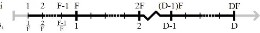
Figure 3.1: Setup of observation locations on a line for analysis under the hybrid asymptotic framework.
3.1
Equally-Spaced Lattice Construction
In order to unify the expanding domain and infill frameworks, which have often been treated separately
in the literature, we will set up our equally-spaced lattice in a way that allows for analysis under the
hybrid framework. To do so, we will consider an interval of length D, where each one-unit length is subdivided intoF subintervals. This corresponds to the observation locations being defined as si≡ Fi fori∈ {1, ...,DF}, which is illustrated in Figure 3.1. Note that unlike Zhang and Zimmerman (2005), we will exclude the points0=0 in all of our derivations, but this will not affect the resulting asymptotic distribution (2.1). This exclusion is simply for convenience when working with the composite marginal
blockwise likelihood in Section 3.4.
To prove that our setup is suitable under the various geostatistical asymptotic frameworks, we will show
that they conform to Definition 1.11. From the notation used in Definition 1.11, the location furthest
away from a givensj is∆j,N=max
n
j−1 F ,D−
j F
o
units away, and the closest observation isδj,N=1/F units away. Consequently,
∆DF= min 1≤j≤DFmax
nj−1 F ,D−
j F
o
→∞ asD→∞,
and
δDF= max 1≤j≤DF
1
F →0 asF→∞.
3.2
Full Likelihood
The Fisher information matrix for the one-dimensional nuggetless exponential covariance Gaussian
pro-cess is presented in Zhang and Zimmerman (2005) under the expanding domain framework. What
follows is an outline of the derivation of this matrix under the more general hybrid framework.
3.2.1 Derivation of the Inverse Fisher Information Matrix
Lety= (y(s1),y(s2), ...,y(sDF))T ∼N(0,Σ0), whereΣ0,i j =cov[y(si),y(sj)] =σ20e−α0|si−sj|. The full log-likelihood can be written as
`(σ2,α;y) =−1
2log|Σ| − 1 2y
T
Σ−1y+constant, (3.1)
where
Σ=σ2
1 e−αF e− 2α
F . . . e−
(DF−2)α F e−
(DF−1)α F
e−αF 1 e− α
F . . . e−
(DF−3)α F e−
(DF−2)α F
e−2Fα e−αF 1 . . . e−
(DF−4)α F e−
(DF−3)α F
..
. ... ... . .. ... ...
e−(DF−F2)α e−
(DF−3)α F e−
(DF−4)α
F . . . 1 e−αF
e−(DF−F1)α e−
(DF−2)α F e−
(DF−3)α
F . . . e−αF 1
In order to find the determinant|Σ|and inverseΣ−1, Kac et al. (1953) derived the Cholesky
decompo-sitionΣ=LDLT, whereLis unit lower triangular andDis diagonal. They showed that
L=
1 0 0 . . . 0
e−Fα 1 0 . . . 0
e−2Fα e−αF 1 . . . 0
..
. ... ... . .. ...
e−(DFF−1)α e−
(DF−2)α F e−
(DF−3)α
F . . . 1 ,
andD=σ2diag 1,1−e− 2α
F ,1−e− 2α
F , . . . ,1−e− 2α
F
| {z }
DF−1 times
. The determinant ofΣis then
|Σ|=|L||D||LT|=|D|= (σ2)DF(1−e− 2α
F )DF−1. (3.3)
To find the inverse ofΣ, we first invertLto obtain
L−1=
1 0 0 . . . 0 0
−e−αF 1 0 . . . 0 0
0 −e−αF 1 . . . 0 0
..
. ... . .. ... ... ...
0 0 0 . .. 1 0
0 0 0 . . . −e−Fα 1
so that
Σ−1= (L−1)TD−1L−1= 1
σ2(1−e−2Fα)
1 −e−αF 0 . . . 0 0
−e−αF 1+e− 2α
F −e−Fα . . . 0 0
0 −e−αF 1+e− 2α
F . .. 0 0
..
. ... . .. . .. . .. ...
0 0 0 . .. 1+e−2Fα −e−αF
0 0 0 . . . −e−αF 1
,
or in terms of the entries,
{Σ−1}i j=
1
σ2 1−e−2Fα
1, i= j∈ {1,DF}
1+e−2Fα, i= j∈ {2,3, ...,DF−1}
−e−Fα, |i−j|=1 0, otherwise
.
Using (3.3), we can then rewrite (3.1) as
`(σ2,α;y) =−DF 2 log(σ
2)−DF−1
2 log(1−e −2α
F )−1 2y
TΣ−1y+constant,
so the score function is given by
sc(σ2,α;y) = ∂` ∂σ2 ∂` ∂α = −DF 2σ2 −
1 2y
T∂Σ−1 ∂σ2 y
−(DF−1)e−
2α F F 1−e−2Fα
−12yT∂Σ∂α−1y .
Note that the system of equations sc(σ2,α;y) =0cannot be solved analytically, so the maximum
likeli-hood estimates ˆσ2and ˆαneed to be found numerically.
ma-trix. Firstly, we require the (observed) information matrix:
info(σ2,α;y) =−
∂2` ∂(σ2)2
∂2` ∂σ2∂α
∂2` ∂σ2∂α
∂2` ∂α2 =
−DF2
σ4+ 1 2y
T∂2Σ−1 ∂(σ2)2y
1 2y
T∂2Σ−1 ∂σ2∂αy 1
2y T∂2Σ−1
∂σ2∂αy
2(DF−1)e−2Fα F2 1−e−2α
F
2+12yT∂ 2Σ−1
∂α2 y .
In order to compute the expectations of these terms, we will make use of the following lemma:
Lemma 3.1(Expectation of a quadratic form) Letx= (x1, ...,xn)T follow a joint distribution with zero mean and covariance matrixΣ. Also, letU= (ui j)n×n. ThenE[xTUx] =tr(UΣ), where tr(·)is the trace operator.
Proof:E[xTUx] =∑ni=1∑nj=1ui jE[xixj] =∑in=1∑nj=1ui jΣji=∑ni=1(UΣ)ii=tr(UΣ).
By applying this lemma to the top-left element of the information matrix, we obtain
E "
−DF
2σ4+ 1 2y
T∂2Σ−1 ∂(σ2)2y
#
=−DF
2σ4+ 1 2tr
∂2Σ−1 ∂(σ2)2Σ
!
=−DF
2σ4+ 1 2tr
2 σ4Σ
−1Σ !
=−DF
2σ4+ DF
σ4 = DF 2σ4.
In this example, computation of the second-order partial derivative with respect toσ2was
straightfor-ward since it only appears as a multiplicative term. Calculation of the other terms follows in a similar
manner, but requires slightly more involved algebraic manipulation. Ultimately, one can derive the entire
(expected) Fisher information matrix, which is
I(σ2,α;y) =E[info(σ2,α)] = DF 2(σ2)2
(DF−1)e−2Fα σ2F 1−e−2Fα
(DF−1)e−2Fα σ2F 1−e−2Fα
(DF−1)e−2Fα 1+e−2Fα F2 1−e−2α
F 2 . (3.4)
withDFobservations instead ofDF+1. The inverse of the Fisher information matrix is then given by
I(σ2,α)−1= 1
1−e−2FαDF+2e− 2α
F
2(σ2)2 1+e− 2α
F −2σ2F 1−e− 2α
F
−2σ2F 1−e−2Fα F2
DF 1−e−2Fα 2
(DF−1)e−2Fα
. (3.5)
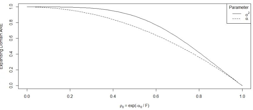
3.2.2 Asymptotics
Under expanding domain asymptotics (D→∞andFfixed), each of the terms in (3.5) converges to 0 at a rate of 1/D, and so the maximum likelihood estimators ofσ2andαare consistent. Furthermore, the attainment of asymptotic normality can be verified by applying Theorem 2.2. Specifically, we have the
set of all unique displacements
H
N≡ {|si−sj|;i,j∈ {1,2, ...,N}}={0,F1,F2, ...,DFF−1}and covariance functionCy(h) =σ2e−α|h|, so limD→∞∑h∈HN|Cy(h)|=limD→∞∑DFj=0−1σ2e−αj
F is a convergent geometric
sum, and the first and second-order partial derivatives ofCy(h)also form convergent sums or equal zero. Thus, by noting that
lim
D→∞DFI(σ 2,
α)−1=
2(σ2)2 1+e
−2α F 1−e−2Fα
−2Fσ2
−2Fσ2 F2(e2Fα−1)
≡V(σ2,α), (3.6)
an asymptotic distribution for large values ofDis
√
DF
ˆ
σ2ML−σ20 ˆ
αML−α0
·
∼N(0,V(σ20,α0)).
This matches up with the work of Zhang and Zimmerman (2005) and (2.1).
In contrast, under infill asymptotics (F →∞andDfixed), both ˆσ2ML and ˆαML do not conform to the usual asymptotic behaviour of maximum likelihood estimators. This can be shown by taking the limit
As an example, the limit of the top-left element of the inverse Fisher information matrix can be found as
follows:
lim F→∞
2(σ2)2 1+e−2Fα 1−e−2FαDF+2e−
2α F
=lim δ→0
2δ(σ2)2(1+e−2αδ)
(1−e−2αδ)D+2δe−2αδ
=lim δ→0
2δ(σ2)2(1+ (1−2αδ+2α2δ2+
O
(δ3)))(1−(1−2αδ+2α2δ2+
O
(δ3)))D+2δ(1−2αδ+2α2δ2+O
(δ3))=lim δ→0
2(σ2)2(δ−αδ2+α2δ3+
O
(δ4))(αδ−α2δ2+
O
(δ3))D+δ(1−2αδ+2α2δ2+O
(δ3))=lim δ→0
2(σ2)2(1+
O
(δ))(α+
O
(δ))D+1+O
(δ) = 2(σ2)2 αD+1.By applying the same procedure to each of the terms in (3.5), we obtain
lim F→∞I(σ
2,
α)−1= 2 αD+1
(σ2)2 −ασ2
−ασ2 α2
. (3.7)
Here, none of the elements converge to zero, so the consistency of ˆσ2MLand ˆαMLis not guaranteed (Ying,
1991). Some insight into why this is the case can be gained by considering the interaction between the
variability of estimation in ˆσ2ML and the true value ofα. In both (3.6) and (3.7), which correspond to
the limit of the inverse Fisher information matrix under the expanding domain and infill approaches
respectively, the top-left element is a monotone decreasing function ofα. This suggests that if there is
a particularly strong correlation between nearby observations (α0≈0), then ˆσ2ML will be subject to a
higher level of variability than if the observations have a low correlation (α0large). Hence, in the case
of infill asymptotics where observations are taken near each other and are thus strongly dependent, each
additional observation that is sampled becomes far less informative about the true value ofσ2.
Another factor which contributes to the behaviour of infill asymptotics in this case is the fact that both
σ2andαare being estimated simultaneously. If we assume thatαis known, then we need only consider
we assume thatσ2is known, then we need only consider the bottom-right element in (3.4) to find the
asymptotic variance of ˆαML, which also converges to zero under both asymptotic frameworks. Based
on this, the asymptotic distributions for ˆσ2MLand ˆαMLas shown by Ying (1991) can be derived, which
results in (2.2) and (2.3). However, we know from (3.7) that convergence of the variance does not occur
under infill asymptotics when both parameters are unknown. This can be attributed to the fact that having
to estimate both parameters simultaneously effectively leads to them competing for information in the
data.
In order for the usual asymptotic results to hold while using an infill sampling scheme, it will be
nec-essary to consider the hybrid framework where the domain of sampling will expand at the same time.
From (3.7), it is clear that as long as D→∞, irrespective of the rate, the inverse Fisher information matrix will approach the zero matrix. This suggests that, when the domain is of a finite size, there is
asymptotically insufficient information aboutσ2andαto achieve consistent estimation simultaneously.
3.3
Composite Conditional 2-Nearest Neighbours Likelihood
For the classes of composite conditional likelihood that we have highlighted in Section 2.3, we can first
consider the composite conditionalK-sequential neighbours likelihood. It is well-known (see Cressie and Wikle (2011, p. 169) for instance) that the one-dimensional exponential covariance Gaussian process
on an equally-spaced lattice can be equivalently expressed as an autoregressive process of order 1 from
time series, wherey(s1)∼N(0,σ2)and
(y(si)|y(s1), ...,y(si−1)) d
= (y(si)|y(si−1))∼N(e− α
Fy(si−1),σ2(1−e− 2α
F )), 1<i≤N=DF.
Since this process satisfies the Markov property, the constructed composite likelihood will be equivalent
is available on a number line. Thus, a potential issue with the composite conditional K-sequential neighbours likelihood is the choice of observation sequence, which is more prominent in two or higher
dimensions. In light of this, we shall investigate the statistical performance of the composite conditional
K-nearest neighbours likelihood as its construction is far less ambiguous.
3.3.1 Construction of the Composite Likelihood
In order to find conditional distributions of Gaussian random variables, we can apply the following
lemma, as presented for example by Eaton (1983, p. 116-117):
Lemma 3.2(Conditional Gaussian distribution) Letx1∼N(µ1,Σ11), x2∼N(µ2,Σ22), andx≡
(xT
1,xT2)T∼N(µ,Σ), whereµ= (µT1,µT2)T and Σ=
Σ11 Σ12
Σ21 Σ22
.
Then(x1|x2)∼N(µ¯,Σ¯), where ¯µ=µ1+Σ12Σ−221(x2−µ2)and ¯Σ=Σ11−Σ12Σ−221Σ21.
Now under the one-dimensional exponential covariance Gaussian process on an equally-spaced lattice,
it can shown using this lemma that
(y(s1)|y(s2), ...,y(sK+1)) d
= (y(s1)|y(s2))∼N(e−Fαy(s2),σ2(1−e− 2α
F )), (3.8)
(y(sDF)|y(sDF−1), ...,y(sDF−K)) d
= (y(sDF)|y(sDF−1))∼N(e− α
Fy(sDF−1),σ2(1−e− 2α
F )), (3.9)
and forK≥2 and 1<i≤N−1=DF−1 that
(y(si)|K-nearest neighbours) d
= (y(si)|y(si−1),y(si+1))∼N
e−Fα(y(si−1) +y(si+1)) 1+e−2Fα
,σ21−e −2α
F
1+e−2Fα !
.
(3.10)